HAL Id: hal-00415736
https://hal.archives-ouvertes.fr/hal-00415736v2
Preprint submitted on 30 Nov 2009
HAL is a multi-disciplinary open access
archive for the deposit and dissemination of
sci-entific research documents, whether they are
pub-lished or not. The documents may come from
teaching and research institutions in France or
abroad, or from public or private research centers.
L’archive ouverte pluridisciplinaire HAL, est
destinée au dépôt et à la diffusion de documents
scientifiques de niveau recherche, publiés ou non,
émanant des établissements d’enseignement et de
recherche français ou étrangers, des laboratoires
publics ou privés.
Probing magnetic fields with multi-frequency polarized
synchrotron emission
Jerome Thiebaut, Simon Prunet, Christophe Pichon, Eric Thiébaut
To cite this version:
Jerome Thiebaut, Simon Prunet, Christophe Pichon, Eric Thiébaut. Probing magnetic fields with
multi-frequency polarized synchrotron emission. 2009. �hal-00415736v2�
Probing magnetic fields in volume
with multi-frequency polarized synchrotron emission.
J. Thi´ebaut
1, S. Prunet
1⋆, C. Pichon
1,3and E. Thi´ebaut
21Institut d’astrophysique de Paris (UMR 7095), 98 bis boulevard Arago , 75014 Paris, France.
2Centre de Recherche Astronomique de Lyon (UMR 5574), 9 avenue Charles Andr´e, 69561 Saint Genis Laval Cedex, France. 3Service d’Astrophysique, IRFU, CEA-CNRS, L’orme des meurisiers, 91 470, Gif sur Yvette, France.
November 30, 2009
ABSTRACT
We investigate the problem of probing the local spatial structure of the magnetic field of the interstellar medium using multi-frequency polarized maps of the synchrotron emission at radio wavelengths. We focus in this paper on the three-dimensional reconstruction of the largest scales of the magnetic field, relying on the internal depolarization (due to differential Faraday rotation) of the emitting medium as a function of electromagnetic frequency. We argue that multi-band spectroscopy in the radio wavelengths, developed in the context of high-redshift extragalactic HI lines, can be a very useful probe of the 3D magnetic field structure of our Galaxy when combined with a Maximum A Posteriori reconstruction technique.
When starting from a fair approximation of the magnetic field, we are able to recover the true one by using a linearized version of the corresponding inverse problem. The spectral analysis of this problem allows us to specify the best sampling strategy in electromagnetic fre-quency and predicts a spatially anisotropic distribution of posterior errors. The reconstruction method is illustrated for reference fields extracted from realistic magneto-hydrodynamical simulations.
1 INTRODUCTION
The problem of studying the magnetic field structure of our Galaxy using measurements of the synchrotron emission of high energy electrons in the Galactic magnetic field is an old one (Ginzburg & Syrovatskii 1965; Ruzmaikin et al. 1988; Beck et al. 1996). The fact that the emitting medium is itself magnetized induces a differential Faraday rotation of the different emission planes transverse to the line of sight, resulting in a well known de-polarization effect of the integrated emission that depends strongly on the electromagnetic frequency. This effect, described in the first place by Burn (1966) in the case of a constant magnetic field, has been further studied in semi-analytically for given functional forms of the magnetic field; it has also been studied from the statistical point of view in some asymptotic regimes (see e.g. Sokoloff et al. 1998). In the present work, we want to consider the more am-bitious problem of using this depolarization effect, together with the solenoidal character of the magnetic field, to reconstruct the magnetic field structure from a set of polarized maps of the syn-chrotron emission of an ionized medium at different electromag-netic frequencies. With the upcoming prospect of detailed Multi-band spectroscopy in the radio wavelengths (R¨ottgering 2003; Furlanetto & Briggs 2004), developed in the context of Galactic and high-redshift extragalactic HI lines, this type of investigation should become possible.
A statistical inference of the measurement of the Galac-tic magneGalac-tic field correlator as a function of scale from multi-frequency polarization measurements has already been success-fully achieved by Vogt & Enßlin (2005) in the case of the Fara-day rotation of the polarized light from background objects by the
intra-cluster magnetized plasma. In this case, there is no depolar-ization effect due to differential Faraday rotation, and the relation-ship between the measured polarization at a given frequency and the polarization of light in the source plane is linear in the (longitu-dinal) magnetic field strength. The linearity of the problem makes the statistical analysis tractable in the former case. In the case that we investigate, the emitting and the rotating medium are the same, which results in depolarization effects of the emitted light. More-over, the synchrotron emissivity itself depends non-linearly on the field strength transverse to the line of sight. The reconstruction of the magnetic field structure from the polarization data is in this case a non-linear inverse problem. Finally, we must note that to address the full problem of reconstruction of the magnetic field from the depolarized synchrotron emission we need in principle knowledge of both the thermal electron spatial distributionne and the
spa-tial distribution of cosmic ray electronsnr, when, in comparison,
the inference of the magnetic energy spectrum from the rotation measures of background sources only requires knowledge of the thermal electron distribution.
In a first attempt at reconstructing the magnetic field, and for the sake of clarity, we make the assumption that the fluctuations of the thermal and cosmic ray electrons can be neglected compared to the fluctuations in the magnetic field itself. This assumption, if physically unrealistic, allows us to show the specific influence of the magnetic field statistical properties on the quality of the re-construction. In the first sections, we thus consider the electronic distributions (both thermal and relativistic) as constant, and discuss the reconstruction of the magnetic field using only the leading cou-pling coefficient in the equation of radiative transfer. In the (thin medium, strong rotativity) limit that we assume for this work, this
leading term is the usual Faraday term, responsible for the rotation of the plane of polarization. We will assume that the Faraday co-efficient is dominated by the thermal electrons, which is a reason-able assumption in non-relativistic astrophysical plasmas. Finally, in section 4, we relax the unrealistic assumption of a constant ther-mal electrons density, and show that our method can still be used to reconstructed the magnetic field when the electronic density is spa-tially varying but known a priori, using simulated data sets from a magneto-hydrodynamical (MHD) simulation.
This paper is organized as follows: in section 2 we discuss the fonctional dependence of the polarization of the synchrotron emission and its variation with electro-magnetic frequency on the underlying magnetic field. We present a discretized version of this functional dependence that will be useful in the context of the re-construction from discrete polarization data. In section 3 we inves-tigate the reconstruction of the magnetic field from simulated multi-frequency polarized data, when the functional dependence on the magnetic field has been linearized around a ”mean” field. Taking advantage of the linear nature of this approximate problem, we give a strategy for choosing the best electromagnetic frequencies of ob-servation, and investigate the statistical anisotropy of the magnetic field reconstruction errors. Finally, in section 4, we investigate the validity of the linearization procedure used in the precedent section, as a function of the quality of our prior knowledge of the magnetic field structure. We show how the approximate, linearized inverse problem investigated in this work could be used as a building block of the fully non-linear reconstruction problem. We emphasize that any gradient-based non-linear minimization algorithm can be de-composed into linear sub-problems, thus justifying the study of the linearized problem. In this context, we investigate how the condi-tioning of the linearized problem varies with the properties of the reference magnetic field around which the problem is being lin-earized. In particular it is illustrated on a realistic reference field from a MHD simulation. Finally, using the same MHD simulation data, we show that our method can deal with a non-constant elec-tronic density, provided it is known a priori. In section 5, we sum-marize the main results of the paper, recalling the main simplifying assumptions used to derive them (notably the assumed-known elec-tronic density hypothesis) and discuss how this assumption could be possibly alleviated by additional data (e.g., Hα, free-free) or by
using second-order coupling terms involving the circular polariza-tion in the case of relativistic sources (see C). We conclude on how the different results of the paper could be used to tackle the fully non-linear reconstruction of the magnetic field.
2 POLARIZED EMISSION
Our objective is to recover the magnetic field given observed po-larization maps at different wavelengths. We tackle this ill-posed problem by means of an inverse problem approach (Tarantola 1987) which involves recovering the magnetic field that gives a polariza-tion consistent with the observapolariza-tions while obeying some a priori properties. These priors are strict constraints, such as∇ · B = 0,
to insure that the sought field is physically meaningful and a reg-ularization to lever the degeneracies of the inverse problem while avoiding artifacts due to noise amplification. We first derive the di-rect model of the polarization given the magnetic field and then introduce the inverse problem approach in a Bayesian framework.
2.1 Direct model
We only consider here the Faraday rotation in the transfer equation, and neglect all other coupling terms. In this case, the transfer equa-tion of the Stokes parameters of linear polarizaequa-tion(Q, U ) can be
integrated formally. We assume here that the density of electrons is constant, or that its fluctuations are only important on scales that are not considered here.
Consider a slab of ionized magnetized medium of widthL
which is emitting synchrotron radiation. The polarized emission, as a function of frequency, integrated over the line of sight then reads (Sokoloff et al. 1998):
P ≡ Q + i U = Z
ǫ(r) e2 i ψ(r)dz , (1) withQ and U are the usual Stokes parameters, ǫ(r) the synchronton
emissivity which obeys:
ǫ(r) = A nr(r) |B⊥(r)|
γ+1
2 ν−γ−12 , (2)
andψ(r) the sum of the Faraday rotation and the primordial
orien-tation: ψ(r) = π/2 + arctan (By/Bx) +K ν2 Z 0 z neBzdz′, (3)
where r≡ (x, y, z) = (x⊥, z) is the coordinate in the slab, ν is
the frequency, andB = (Bx, By, Bz) = (B⊥, Bz) is the magnetic
field. In equation (3),K reads: K = q 3 e 8 π2m2 ec ǫ0 , (4)
while, in equation (2),A is given by A = √ 3 Eγ0q3 e 16 π ǫ0mec „ 3 qe 2 π m3 ec4 «γ−12 Γ„3 γ − 1 12 « Γ„3 γ + 1 12 « ,
whereE0is the energy scale of the relativistic electron spectrum,
meand qestand for the mass and the charge of the electron,ne
andnrare the thermal and relativistic electron densities supposed
constant, while the exponentγ stands for the spectral index of the
cosmic ray electrons,c is the speed of light, ǫ0is the electric
per-mittivity andΓ is the Euler gamma function. The lengths are in
kilo-parsec (kpc) and so the density in kpc−3, the magnetic fields in micro-Gauss (µG) and the frequencies in giga-Hertz (GHz).
Re-expressing the intrinsic polarization phase in terms of powers of the magnetic field components, we get the following expression for the polarization: P (x⊥, ν) = A ν− γ−1 2 Z 0 −∞ nr(x⊥, z)`Bx2+ By2 ´γ−34 (x ⊥, z) ×`B2 x− B2y+ 2 i BxBy´ (x⊥, z) × exp„ 2 i Kν2 Z0 z (neBz)(x⊥, z′′) dz′′ « dz . (5) As real data come in discrete form, let us discretize this expression by replacing all integrals with sums, assuming a regular discretiza-tion grid that will be defined more precisely below. Equadiscretiza-tion (5) then reads P (x⊥, ν) = A h ν− γ−1 2 X z nr(x⊥, z)`B2x+ By2 ´γ−34 (x ⊥, z) ×`B2 x− By2+ 2 i BxBy´ (x⊥, z) × exp 2 i K hν2 X z′ θH(z′− z) (neBz)(x⊥, z′) ! . (6)
HereθH is the Heaviside function (θH(x) = 1 for x ≥ 0 and 0
elsewhere), andh the discretization length along z. Equation (6) is
formally a function of B ≡ {(Bx, By, Bz)}rwhere we use bold
symbols to represent the discretized vector fields and r is a triple index spanning the magnetized volume on a regular cubic mesh with cell sizeh.
The solution to the inverse problem will be obtained by means of minimization of some merit function (as explained in what fol-lows), we therefore need to compute the partial derivatives of the polarization with respect to the magnetic field. Let us first com-pute the derivatives with respect to the transverse components of the field: ∂P (x⊥, ν) ∂Bx(r′) = δD(r − r ′) A n r(r′) h ν− γ−1 2 (B2 x+ B2y) γ−7 4 (r′) ×»1 + γ2 B3x+7 − γ 2 B 2 yBx+ i (γ − 1) B2xBy+ 2 i B3y – (r′) × exp 2 i K hν2 X z′′ θH(z′′− z′) (neBz)(x′⊥, z′′) ! , (7)
with r = (x⊥, z), r′ = (x′⊥, z′) and δDDirac’s delta function.
The derivative with respect toByfollows closely, with the square
bracket term becoming:
» −1 + γ2 B3y−7 − γ 2 B 2 xBy+ i (γ − 1) BxBy2+ 2 i B3x – (8) which corresponds to aπ/2 rotation in the plane perpendicular to
the LOS. We see that in both cases the phase term is unaffected since it is only a function of the longitudinal magnetic field com-ponent Bz. Finally let us compute the derivative with respect to
Bz: ∂P (x⊥, ν) ∂Bz(r′) = δD(x⊥− x′⊥)2iKAh2ν− γ+3 2 ×X z nr(x′⊥, z)(Bx2+ By2) γ−3 4 (B2 x− By2+ 2iBxBy)(x′⊥, z) ×θH(z′− z) exp 2iKh ν2 X z′′ θH(z′′− z)( neBz)(x⊥, z′′) ! . (9)
We note that here the phase term, not the emissivity layer term, is involved. The caseγ = 3 is detailed in Appendix A and leads to a
simplification of the above equations.
2.2 Maximum A Posteriori formulation
From the direct model, we can express the observed data as:
dm= P`(x⊥, ν)m, B´ + em, (10)
withm an index which spans the mixed frequency
position-on-the-sky cube,(x⊥, ν)mthe corresponding coordinates, B the actual
magnetic field andeman error term which accounts for noise and
model approximations. Using vector notation, equation (10) simpli-fies to: d= P(B) + e with d = {dm} the vector collecting all the
observations, P(B) = {P`(x⊥, ν)m, B´} and e = {em}. Our
inverse problem is to recover the magnetic field vector, B, given some noisy measurements of the polarization, d. Due to the un-known errors in equation (10) and to possible strict degeneracies of the direct model, there is not a unique magnetic field that yields a polarization consistent with the observations. We therefore need some means to select a unique solution and, hopefully, the best one given the data.
Probabilities provide a consistent framework to define such
a solution; we thus define the sought magnetic field as being the most likely given the observations. It is the one which maximizes the posterior probability:
BMAP= arg max
B P(B|d) ,
(11) and which is termed as the maximum a posteriori (MAP) solution (see e.g. Pichon & Thi´ebaut 1998). By Bayes’ theorem,P(B|d) = P(d|B) P(B)/P(d), and since P(d) does not depend on the
sought parameters B, this amounts to maximizingP(d|B) P(B).
The termP(d|B) is the likelihood of the data given the model,
while the termP(B) accounts for any a priori knowledge about the magnetic field. We can anticipate two types of priors: (i) the strict constraint that, to be physically meaningful, the field should be solenoidal:∇B = 0; (ii) some so-called regularization
con-straint to overcome the ill-conditioning of the inverse problem and to enforce the unicity of the solution. Without loss of generality, we state that the probabilities writes:
P(d|B) = κ1 exp`−12L(B)´ , (12)
P(B) = (
κ2 exp`−12R(B; µ)´ , if ∇B = 0,
0 otherwise. (13)
where the factorsκ1 andκ2do not depend on B andµ accounts
for parameters to tune the regularization. Finally, taking the log-probabilities and discarding constants, the maximum a posteriori magnetic field writes:
BMAP= arg min
B,∇B=0Q(B) ,
(14) with:
Q(B) = L(B) + R(B; µ) , (15) which is the objective function. Before going into the details of the expressions ofL(B) and R(B; µ) we can already note that the
solution BMAPwill depend on the data d and on the
regulariza-tion parametersµ. The value of µ can be chosen, e.g., to provide
the best bias-variance compromise on the sought solution (Wahba 1990; Golub et al. 2000).
2.2.1 Likelihood
Assuming Gaussian statistics for the noise and model errors, the likelihood of the data is the so-calledχ2and writes:
L(B) =`d − P(B)´⊤· C−1n ·`d − P(B)´ (16)
with Cnthe covariance matrix of the errors. There is a slight issue
here because we are dealing with complex values. Since complex numbers are just pairs of reals, complex valued vectors such as d,
P(B) and e can be flattened into ordinary real vectors (with
dou-bled size) to use standard linear algebra notation. This is what is assumed in equation (16). Under these conventions, the covariance matrix of the errors writes Cn = he · e⊤i with⊤to denote
trans-position.
2.2.2 Regularization
The regularization termR(B; µ) implements loose constraints to
avoid over-fitting the data and enforce local unicity of the solution (see section 4.3). Requiring that the magnetic field be as smooth as possible (while being consistent with the data) matches these requirements and is supported by physics since the magnetic field
should have no discontinuities. To simplify further computations, we choose the following particular expression of the regularization
R to favor the smoothness of the field: R = µsk∆α/4Bk2∝ µs
X
k
|k|α| ˆB|2, (17) which scales as the integrated norm of the spatial Laplacian of the field to the powerα/4. For a periodic field, this generic smoothing
penalty is diagonal in Fourier space. In addition, if the model B is Gaussian and scale invariant, thenα may be chosen to be the power
law index of the power spectrum| ˆB|2k of the field. In this case,
choosing the specific value of the hyperparameter,µs= 1/| ˆB|2k=1,
the MAP solution correspond to the minimal variance Wiener fil-tered data.
2.2.3 Imposing∇B = 0
For simplicity, we assume here that the magnetic field is multi-periodic, with periodL in all three directions. We may then rewrite
the magnetic field as:
B= F−1· ( ˆB⊥1e⊥1+ ˆB⊥2e⊥2) ≡ Π · B , (18)
where F−1 = F†/Nr3and F is the forward DFT operator, (ek≡
k/|k|, e⊥1, e⊥2) form a spherical basis in Fourier space, while
ˆ
B⊥,i, i=1,2 are the projections over that basis of the Fourier
com-ponent, ˆB≡ F · B of the field. Equation (18) defines the projector Π= F−1· (e
⊥⊗ e⊥) · F. Such a field satisfies by construction
k· ˆB≡ 0 , which implies ∇ · B ≡ 0 . (19) In fact, there is a slight complication at the Nyquist frequencies where only one component of the field is free, see appendix B.
Note that the divergence free condition could also be imposed by other means (see e.g. Nocedal & Wright 2006). For instance, by adding a quadratic penalty term likeP
r(∇B) 2
rto the total penalty
Q(B). We however found that, in practice, the projector Π led to
a better conditioned reconstruction problem.
2.3 Implementation
Given equations (16) and (17) the objective function writes:
Q = (P − d)†· C−1n · (P − d) + µsk∆α/4Bk2. (20)
To minimize Q(B), we used a variable metric limited memory optimization method with BFGS updates (Nocedal 1980) called VMLM and implemented in OptimPack1(Thi´ebaut 2002). Finding the optimal solution, equation (14), involves computing the gradi-ent of equation (20) with respect to B. Now differgradi-entiating equa-tion (16) with respect to a magnetic field components we get
∂χ2 ∂Bi = 2 Re » (P − d)†· C−1n · ∂P ∂Bi – , (21) where∂P/∂Bifori = x, y, z are given by equations (7) and (9).
Similarly, differentiating equation (17) with respect to B yields
∂R ∂Bi
= µsF−1·Bˆi|k|α. (22)
The VMLM algorithm is a quasi-Newton method which proceeds by solving successive linear problems. Let us therefore first con-sider in the next section a linearized version of our inverse problem,
1 OptimPack is freely available at
http://www-obs.univ-lyon1.fr/labo/perso/eric.thiebaut/optimpack.html.
which may correspond to a physically motivated problem when a good first guess for the magnetic field is known.
Note finally that equations (7) and (9) imply that∂χ2/∂Bi=
0 atBx = By = 0. Note also that if (Bx, By, Bz) is a solution
to equation (5), so is(−Bx, −By, Bz). Consequently we expect
that theχ2 will be strongly multivalued as a function of B2. The
smoothing penalty should in part prevent a pixel-by-pixel flip of thex and y component. It remains nonetheless to be shown that the
zero divergence condition is sufficient to avoid flipping the field in regions bound by zeros of these two components, if such regions exist. Addressing these issues will be the topic of another paper.
3 LINEARIZATION
Let us first consider the situation when a fairly good guess for the overall magnetic field, B0, is known, on the basis, say of
a first large scale investigation, or via some modelling of the field as a function of the underlying density (e.g. Cao et al. 2006; Kachelrieß et al. 2007). Let us then seek the departure from this guess. It is then legitimate to assume B= B0+ δB, with,
possi-bly (if the prime guess is accurate enough)δB/|B0| ≪ 1, so that
equation (5) becomes:
δP ≡„ ∂P∂B «
B0
· δB, (23) where the tensor∂P/∂Bi is given by its components, equations
(7), (8) and (9), whileδP ≡ P − P(B0). Now equation (23) is
likely to be a much better behaved equation as the linearity warrants convexity of the objective function, hence the formal unicity of the solution.
In this paper, we will address two linear problems in turn, one of academic interest, to understand the properties of the inverse problem at hand, while the second one should allow us to carry realistic reconstructions, in the regime when a fair reference field is known. Specifically, we will first assume that the (noise free) data is in the image of(∂P/∂B)B
0:
d≡ δPL= (∂P/∂B)B0· δB + e , linear problem (I), while for the second problem (the so called Gauss-Newton approx-imation)
d≡ δPPL≡ P − P(B0) + e , pseudo linear problem (II). We investigate the linear problem in this section and the pseudo-linear problem in section 4.
3.1 Linear reconstruction
Let us illustrate our method on a problem of realistic scales. This first simulation is carried on aN3
r grid (Nr = 64) with Nν = 64
frequencies. The reference field B0 is chosen constant and set to
1 µG everywhere for each component, the power spectrum of the
perturbation fieldδB has a power law index α = 2 and its RMS
is0.01. Data are simulated linearly (see section 3) and are noised
with a SNR= 20. Figure 1 illustrates the quality of the
reconstruc-tion. The top panel represents thex and z components along the
LOS (z direction) or transverse (y direction) for a given pixel. As
2 For instance a magnetic loop close to thez axis (where BxandBy∼ 0)
and its mirror image by symmetry along thez axis have the same χ2and
−3.0 −2.5 −2.0 −1.5 −1.0 −0.5 −0.02 −0.01 0.00 0.01 0.02 −3.0 −2.5 −2.0 −1.5 −1.0 −0.5 −0.02 −0.01 0.00 0.01 0.02 z (kpc) Bx ( µ G) Bz ( µ G) Bin Bout −1.5 −1.0 −0.5 0.0 0.5 1.0 1.5 −0.02 −0.01 0.00 0.01 0.02 −1.5 −1.0 −0.5 0.0 0.5 1.0 1.5 −0.02 −0.01 0.00 0.01 0.02 y (kpc) Bx ( µ G) Bz ( µ G) Bin Bout −1.5 −1.0 −0.5 0.0 0.5 1.0 1.5 −1.5 −1.0 −0.5 0.0 0.5 1.0 1.5 0.00 0.00 0.01 0.01 x (kpc) y (kpc) |B| 10.0 20. 100.0 5. 50. 10+1 10+2 10+3 10+4 |k| P(k) Bin Bout SNR=20 Bout SNR=200
Figure 1. Top: input (solid lines) and recovered (dashed lines)x and z components of the field along a LOS (left) and along the y transverse direction (right).
They component and the x direction are not plotted since very close to the x component and the y direction. One can see that the z component is better
reconstructed than thex or y components which is consistant with the variance measurements and the global conditioning of the problem (see section 3.3).
The reconstruction is carried on aNr= 64 grid with Nν= 64 frequency channel. The data are generated linearly (see section 3) with a SNR= 20. Bottom
left: maps of|B| for a transverse section after smoothing of the fields. The green images represents the input field while the superposed white contours show
the recovered one. Bottom right: power spectra of the input field (solid line) and the recovered one (crosses). As expected, the recovered power spectrum is damped at higher frequencies because of the regularization. To illustrate this we added the power spectrum of a reconstruction with SNR=200.
the results for they component and the x direction are similar to
thex component and the y direction, they are not plotted. Here,
the solid lines stand for the input field and the dashed lines for the recovered one. It is clear that the two fields are very similar and that thez component is the best recovered (see section 3.3). The
bottom left panel shows a map of|B| for a transverse section
af-ter smoothing. The smoothing is made by convolving the field with a four pixels full-width at half maximum (FWHM) gaussian. The green features represent the input field and the reconstructed one is shown in the superposed white contours. The bottom right panel shows the power spectra of the input field (solid line) and the
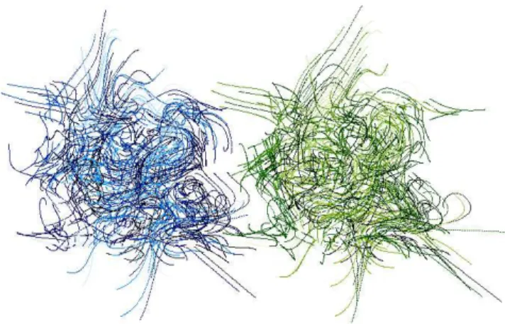
re-covered one (crosses). Finally, figure 2 represents the field lines of the input field (top) and the recovered one (bottom). These fig-ures show that, if the frequencies are correctly sampled (see section 3.2), the linear inverse problem (I) recovers qualitatively well the underlying field. The local and global properties of the field can be reconstructed provided that the linearization remains valid which will be investigated in section 4.
It is of interest to study the conditioning of the linear prob-lem for two reasons (i) to understand the spatial spectral feature of the solution; in particular the biases of the eigenvectors of the linearized problem which induces anisotropy in the distribution of
Figure 2. Field lines of the input (left) and the recovered (right) fields for a
643reconstruction withNν = 64 frequencies. The fields correspond to a
reconstruction with a SNR of 200.
errors around the solution; (ii) to constrain the best sampling strat-egy in order to recover B. Eventually it will also have an impact on our ability to carry out the non linear reconstruction.
The requirements to set up a good conditioning of the global inverse problem can be formulated in steps. First a necessary condi-tion is to make a proper choice of the (electromagnetic) frequency sampling, which can be achieved by looking at a smaller subprob-lem on a given LOS; however, this optimal sampling does not war-rant a good global conditioning; we therefore investigate the qual-ity of the global linear reconstruction by looking at different ele-ments of the reconstruction covariance matrix in (spatial) frequency space. In particular, we will show that the quality of the reconstruc-tion is anisotropic and depends on the components of the field, B, which is confirmed by looking at the eigenvectors of the covariance matrix for a low dimensional problem.
3.2 Conditioning of a line of sight and frequency sampling
One can see easily that in the relation between polarization and magnetic field (equation (5)), each line of sight is independent of the other. The link between them is provided by the solenoidal con-dition. In this subsection we will not consider this condition and the matrix(∂P/∂B)B0becomes block-diagonal. Moreover, the three
components can be separated leading to three different matrices,
(∂P/∂Bx), (∂P/∂By) and (∂P/∂Bz). The field B0 is taken
constant and its modulus set at1 µG. In this case, all blocks are
the same and the study of the conditioning is reduced to the study of threeNν× Nrmatrices withNνthe number of frequencies and
Nrthe number of pixels in thez direction.
Numerical investigations show that the conditioning of
(∂P/∂Bx) depends mainly on the ratio K h neBz/ν2leading to
the conclusion that the conditioning is dominated by the exponen-tial term of equation (7). It follows that(∂P/∂By) has the same
behavior as(∂P/∂Bx) since the exponential terms are the same in
both equations (7) and (8), which is confirmed numerically. Recall that since in this section the reference field is chosen constant, so isBz; therefore the best sampling for the frequencies is
to haveν−2n − νn+1−2 constant, that is a constant step for the squared
wavelength; hence:λ2
n≡ λ20+ (n − 1) ∆λ2withn = 1, . . . , Nν
the index of the frequency/wavelength. So that the complex
expo-nential becomes
e2 i K neBzh m λ2n/c 2
= e2 i K neBzh m λ20/c2e2 i K neBzh m (n−1) ∆λ2/c2 (24)
withm = 1, . . . , Nr the pixel index along the line of sight. The
value of∆λ2must be chosen in such a way that the frequency
de-pendent complex exponentials are uniformly sampled on the com-plex circle. HenceK neBzh Nr(n − 1) ∆λ2/c2must be a
multi-ple ofπ for any n. With L = h Nrthe maximum probed depth and
taking the smallest multiple, this yields:
∆λ2= π c
2
K neBzL
. (25)
With this particular choice, the matrices (∂P/∂Bx) and
(∂P/∂By) take the following form:
(∂P/∂Bx/y)n,m= Cx/yeNriβ
„ λ20+ (n − 1)π K neBzL «γ−14 × „ e−iβe−2iπ(n−1)Nr «Nr−m , (26) whereβ = 2 K neBzh λ20andCx/yis a different constant in the
x and y directions. If the factor`λ2
0+ (n − 1)π/(K neBzL)´
γ−1 4
is set to 1, the matrix is a unitary Vandermond matrix and its con-ditioning is 1 (Cordova et al. 1990).
Accounting for this factor impairs the conditioning but it stays close to unity. The elements of the last matrix,(∂P/∂Bz) are just
geometrical series of the elements of(∂P/∂Bx). Thus, they read:
(∂P/∂Bz)n,m = CzeNriβ „ λ20+K n(n − 1)π eBzL «γ+34 × 1 − exp(−iβ(Nr+ 1 − m)) exp„ −2iπ
Nr (n − 1)(Nr+ 1 − m)
«
1 − exp „
−iβ exp(−2iπN
r(n − 1))
« .
whereCz is yet another constant. At this stage, there is only one
free parameter left, the first frequency λ0. The conditioning of
`∂P/∂Bx/y´ being always close to unity, the value of λ0 must
be chosen in order to minimize the conditioning of(∂P/∂Bz).
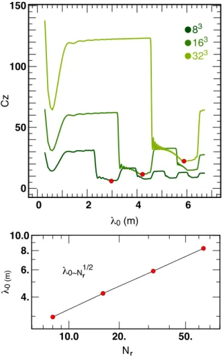
Figure 3 (top panel) represents the conditioning of(∂P/∂Bz)
as a function ofλ0for different grid sizes. The curves are very
simi-lar in shape and the best conditioning is represented by the red dots. In the bottom panel the wavelength providing the best conditioning for(∂P/∂Bz) is plotted as a function of the grid size. It appears
thatλ0 ∝
√
Nr and the precision onλ0 is not really important
since the minimum of the curves are not really marked. These par-ticular choices ofλ0give a conditioning of1.29 for`∂P/∂Bx/y´,
whatever grid size.
3.3 Conditioning of CMAPand a posteriori variances
Let us now investigate the a posteriori variances of different spatial frequencies of the reconstructed field. This covariance matrix can be written as
CMAP= (AT· C−1n · A + C−1B ) −1,
(27) where A ≡ (∂P/∂B0) · Π with Π the projector that
can-cels the divergence (cf. equation (18)) and C−1n and C−1B ≡
0 2 4 6 0 50 100 150 λ0 (m) C z 83 163 323 10.0 20. 50. 10.0 4. 6. 8. N λ0 (m ) λ0~N1/2 r r
Figure 3. Top: conditioning,Cz, of(∂P/∂Bz) as a function of λ0for different grid sizes. The red dots represent the best conditionings. Bottom:
λ0giving the best conditioning as a function of the grid size,Nr. It appears thatλ0∝√Nr.
noise and the signal respectively3. Here we seek ˆCMAP, the Fourier transform of CMAP as we want to understand the relative error
in the amplitude of the spatial modes of B. Because of the po-tential high dimensionality of our problem, the covariance matrix,
ˆ
CMAPis not computed directly. We chose instead to compute the
selected values by solving for ˆB the following equation with a
con-jugate gradient method (CGM, Shewchuk 1994; Nocedal & Wright 2006):
ˆ
WMAP· ˆB= ˆBref. (28)
Here, ˆWMAP= ˆC−1MAPand the solution, ˆB, found by the CGM is ˆ
B= ˆCMAP· ˆBref. (29) The reference field, ˆBref, is equal to1 or ±i for the chosen k
fre-quency and its opposite−k in order to have a real field, and 0
else-where. The elements ˆBkand ˆB−kof the solution are combinations of the covariance of k and−k and the variance of k. It allows us to determine the a posteriori variance of the chosen spatial frequency
3 Throughout this section (unless stated otherwise) we assume thatα is
given by minus the powerspectrum index of the sought magnetic field, and chooseµs = 1/P(k = 1), which corresponds to the minimum variance
solution.
k. To check this method, the same variances were also computed
by the iterative VMLM method. One can check that:
h( ˆBin− ˆBout) · ( ˆBin− ˆBout)†i = ˆCMAP, (30) where† denotes conjugate transposition, ˆBin and ˆBoutstand re-spectively for the input field and the reconstructed one in Fourier space. As expected, the higher the number of iterations, the closer the two estimates of the variance.
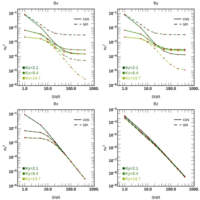
Figure 4 represent the evolution of the a posteriori variance of dif-ferent spatial frequencies k for the difdif-ferent components of the field in different directions (along a LOS or transverse to it) as a func-tion of the SNR. The size of the box isNr = 16 and the number
of frequencies isNν = 16. Figure 5 shows the evolution of the
a posteriori variances of the same frequencies as of figure 4, but as a function of the spectral index,α, of the sought field (for a
SNR= 20). As expected, the variance decreases as the index
in-creases. In Figure 4 the SNR is defined as
SNR = RMS(data)/σn, (31)
withσ2nstanding for the noise variance. The results for theByand
Bzfields in thex direction are not plotted because there are exactly
the same as those in they direction. First note that the variances, σ2
kfor the Bzcomponent of the field are much smaller in
ampli-tude relative to the other components. For the Bxand Byfields, at
low SNR, the Wiener prior is important in the reconstruction, ex-plaining the separation of the three curves corresponding to three different scales. In Fourier space, ˆCB= µ−1s diag(|k|−α) with α
the spectral index of the power spectrum of the input field. If the regularization dominates, ˆCMAP ∼ |k|−α, which corresponds to
the values on the figures when the SNR is low.
For the transverse frequencies (bottom panels), the behaviour of the variances is well understood. At low SNR, the Wiener prior dominates the reconstruction for the Bx and Bycomponents but
not for the Bzone. Increasing the SNR implies increasing the
rel-ative weight of the data compared to the prior. So equation (27) becomes
CMAP∼ (AT· C−1n · A)−1, when SNR → ∞ . (32)
If we assume a Gaussian white noise, Cn= σ2nI with I the identity
matrix, equation (32) becomes
CMAP∼ σn2(AT· A)−1, (33) so CMAP ∝ σn2or given equation (31), CMAP ∝ SNR−2which
is the slope of these curves. Finally, note that there is no symmetry breaking between thex and y directions and between the x and y
components of the field or between the sine and cosine modes in
CMAP.
Now, consider thex and y components of the field along a LOS
(top panels). At low SNR, the Wiener prior still dominate, provid-ing the same value as in the transverse direction. Then, the variance decreases as SNR−2but reaches a threshold and stagnate. It is clear on the figures that there is a symmetry breaking between thex and
they components of the field and a separation between the sine and
cosine modes. At first it may be surprising that the variances reach a threshold since the frequencies have been chosen to provide the best possible conditioning for(∂P/∂B0) along a LOS (see section
3.2). In fact this is a consequence of the solenoidal condition. Re-call that for the global inverse problem, the relevant linear model is A= (∂P/∂B0) · Π, where Π is the projector given by
equa-tion (18). This projector changes the matrix(∂P/∂B0) and adds
off-diagonal terms to the block diagonal matrix considered in the previous subsection. In effect, the solenoidal condition degrades
1.0 10.0 100.0 1000. 10−6 10−5 10−4 10−3 10−2 10−1 Kz=2.1 Kz=8.4 Kz=14.7 cos sin Bx SNR σk 2 1.0 10.0 100.0 1000. 10−6 10−5 10−4 10−3 10−2 10−1 Kz=2.1 Kz=8.4 Kz=14.7 cos sin By SNR σk 2 1.0 10.0 100.0 1000. 10−6 10−5 10−4 10−3 10−2 10−1 Ky=2.1 Ky=8.4 Ky=14.7 cos sin Bx SNR σk 2 1.0 10.0 100.0 1000. 10−9 10−8 10−7 10−6 10−5 10−4 10−3 Ky=2.1 Ky=8.4 Ky=14.7 cos sin Bz SNR σk 2
Figure 4. A posteriori variance of different spatial frequencies k∈ (1, 2, 3) for the different components of the field in different directions (along a LOS or
transverse to it) as a function of the SNR. The size of the box isNr= 16 and the number of frequency is Nν= 16. The top panels correspond to the variation
ofσ2
kfor three different values ofkzwhile the bottom panels correspond to varyingky. The cosine mode (thick line) and sine mode (dashed line) are both
shown. All variances decrease with increasing SNR as expected, although at different rate, see the main text. Note the different amplitude inσ2
kfor the bottom
right panel which shows that the Bzcomponent of the field is better recovered compared to the other components. This reflects the anisotropy of the model A which induces anisotropic reconstruction errors.
the global conditioning relative to the one LOS problem (but recall that without it we have an ill posed problem). In turn this changes the eigen structure of ˆCMAPand therefore its projection in Fourier space.
Indeed, let us compute directly the whole matrix ˆCMAPfor a smaller, more tractableNr = 8 constant reference magnetic field
withNν= 8 frequencies sampled following the procedure defined
in section 3.24. Figure 6 shows the global conditioning of the co-variance matrix CMAPas a function of the SNR. One can see that
the mixing of the LOS has a significant effect on conditioning, even
4 As expected the curves of the variance as a function of the SNR found
previously are recovered exactly with this direct calculation.
though the frequencies were chosen optimally. Figure 6 also shows that at realistic SNR, the global conditioning remains bounded and could be improved, e.g. for the purpose of numerical convergence, by artificially increasing the hyperparameterµs. Note finally that
even though the global conditioning increases with the SNR, the variances all decrease, as expected.
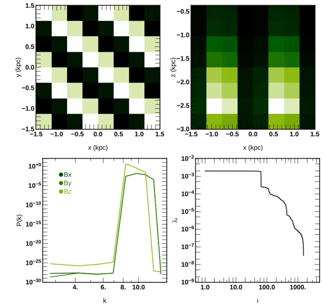
3.4 Eigenspace analysis
In order to understand the plateau on figure 4, let us also explic-itly diagonalize WMAPfor the smaller above-describedNr = 8
problem with a SNR= 20. The corresponding spectrum is plotted
1 2 3 4 5 10−7 10−6 10−5 10−4 10−3 10−2 10−1 Kz=2.1 Kz=8.4 Kz=14.7 cos sin Bx α σk 2 1 2 3 4 5 10−7 10−6 10−5 10−4 10−3 10−2 10−1 Ky=2.1 Ky=8.4 Ky=14.7 cos sin Bx α σk 2
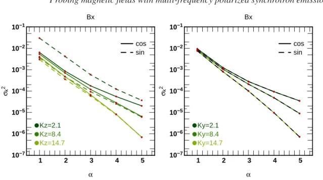
Figure 5. Same as Figure 4 but as a function of the spectral index,α, of δB for a SNR= 20. As expected, the smoother the expected field, the larger α, the
smaller the posterior variances.
is about105 (consistently with what was shown on Figure 6 for
CMAP), but note importantly that there is a cluster of eigenvalues followed by a gap. This gap is consistent with the plateau seen on figure 4. When increasing the SNR, one expects to filter out less and less eigen modes, and therefore to access more and more eigenvec-tors (corresponding to decreasing eigenvalues) in the reconstruc-tion. However, when reaching the gap, although the SNR increases, no more eigenvalues are available for a while. The lower eigenvec-tors, encoding informations on higher frequencies, are not within reach, and the a posteriori variance of these frequencies stagnate, as seen in figure 4. If the SNR increases further, these eigenvalues (and therefore their associated eigenvectors) will be sampled, and we expect that theσ2
kvariances will decrease again5. The
modu-lus of the first eigenvector (associated to the highest eigenvalue) is plotted on the top panels in thex−y (left) and x−z (right) planes.
It is clear on these figures than thex and y directions are isotropic
while thez one is anisotropic for this eigenvector. Moreover, the
component of the power spectra in the bottom left panel show that theBzcomponent clearly differ from the other two components.
However, all of the main eigenvectors do not behave in the same way. Some of them clearly break the symmetry between thex
andy directions or/and between the x and y components leading to
the differences in the curves of figure 4. Finally note that the main eigenvectors are fairly high frequencies fields. So, the a posteriori variances will be smaller for high frequencies than for low ones, which is reflected by the top panels of figure 4.
5 in other words, the plateau seen in the variance per mode in the top panels
reflects the fact that those modes have non zero contributions from the low signal to noise eigen modes (i.e. eigen modes of C−1/2A ·CB·C−1/2A with
low eigen values, where C−1A ≡ AT· C−1 n · A). 0 1 2 3 4 4 6 8 10 Log(SNR) Log(C G )
Figure 6. Global conditioning of the (a posteriori) covariance matrix
CMAPas a function of the SNR. The higher the signal to noise, to more difficult the inversion, but the smaller the covariance a posteriori. The 3D matrix, A= (∂P/∂B0)·Π appears to be more poorly conditioned than its
1D counterpart even though the sampling in electromagnetic frequency was the same as in section 3.2. It remains bounded and within reach of double precision calculation.
4 VALIDITY OF THE LINEAR APPROXIMATION 4.1 Linear and pseudo linear inversion
Let us first carry out a linear inversion of the same pertubative field
δB, with RMS(δB) = 10−3µG, while considering both the linear
(I) and the pseudo linear (II) data sets (see section 3). We work here on aNr = 64 grid, with Nν = 64 frequencies, a constant
refer-ence field of module 1µG and SNR=20. Recall that for the linear
minimum variance solution, the hyperparameterµs= 1/P(k = 1)
(see section 2.2.2), while for the the pseudo linear data set it may be tuned. Figure 8 top panel shows the inputz component for the
in-put field (solid line) along a given LOS and the outin-put ones (dotted
line for the linear data,δPLand dashed line for the pseudo
lin-ear,δPPL) while the bottom panel shows the different power
spec-tra. As previously, the field recovered from linearized data sets fits quite well the input one. The recovered pseudo linear field, though
−1.5 −1.0 −0.5 0.0 0.5 1.0 1.5 −1.5 −1.0 −0.5 0.0 0.5 1.0 1.5 x (kpc) y (kpc) −1.5 −1.0 −0.5 0.0 0.5 1.0 1.5 −3.0 −2.5 −2.0 −1.5 −1.0 −0.5 x (kpc) z (kpc) 10.0 4. 6. 8. 10−30 10−25 10−20 10−15 10−10 10−5 10+0 Bx By Bz k P(k) 1.0 10.0 100.0 1000. 10−9 10−8 10−7 10−6 10−5 10−4 10−3 10−2 i λi
Figure 7. Top panels: maps of the modulus of the field corresponding to the first eigenvector of WMAPin thex−y (left) and x−z (right) plans for a 83
constant reference magnetic field withNν= 8 frequencies sampled as explained in section 3.2 with a SNR= 20. The first eigenvector appears to be isotropic
inx and y and anisotropic in the z direction. Bottom left: power spectra of the three components of this eigenvector. The anisotropy of the z component is
clearly visible and in good agreement with the results found in section 3.1 (figure 1) and 3.3 (figure 4). Bottom right: spectrum of the eigenvalues of WMAP.
somewhat different from the linear one, remains fairly close to the original field. The corresponding powers pectra are also shown on Figure 8 and confirm that the recovered field in setting (II) is quan-titatively redder.
4.2 Second order residuals
Let us now study the second order residuals to quantify the do-main of validity of the linearization. For this purpose, we subtract to the total polarization its zero and first order expansion to obtain (P−P0−(∂P/∂B)B0 ∝ δB2) and we divide this quantity by the
first order term (P− P0 ∝ δB). Figure 9 represents the average
of this quantity as a function of RMS(δB). Here the perturbation
consist of a single frequency and single component field. The solid
lines represent the results obtained with aBxcomponent along the
LOS at the lowest mode, while the dashed lines correspond to the lowest transverse mode of theBzcomponent. The dark curves
rep-resent the real part,Q, of the polarization while light ones stand for
the imaginary partU (see equation (1)). At very low RMS(δB),
numerical noise dominate but decreases as the RMS increases. Af-ter reaching a minimum, note that the quantity plotted increase as RMS(δB) since ∝ δB2/δB and thus ∝ δB. As expected, the
lower the RMS(δB), the better the linear approximation and the
better the reconstruction. Note also the significant amplitude dif-ference between the Bz and Bxcomponents; we interpret this as
a difference between the second derivatives of the field, which in turn, impairs the accuracy of the linearization for thez component.
This should not be a limitation when carrying the non linear re-construction using a method such as VMLM, as the amplitude of the subsequent changes in the magnetic field will be scaled by the inverse second derivatives.
−3.0 −2.5 −2.0 −1.5 −1.0 −0.5 −0.001 0.000 0.001 0.002 Bin Bout L Bout PL z (kpc) Bz ( µ G) 10.0 20. 100.0 200. 5. 50. 0.001 0.01 0.1 1.0 10.0 100.0 1000. Bin Bout L Bout PL |k| P(k)
Figure 8. Top: Bz along a LOS for the input field (solid line) and for
the recovered fields with linear data,δPL(dashed line) and pseudo linear ones,δPPL(dotted line) (see section 3). Bottom: power spectra of these three fields. Note that the power spectrum of the reconstructed field from the pseudo linear data set is steeper.
4.3 Towards the non linear problem
Up to now, we have only considered the situation where B0 was
assumed to be constant. What happens to the conditioning when we add spatial frequencies to B0or/and over ne? It is easy to see
that adding transverse frequencies to thex or the y component of B will not change the conditioning of a LOS. Indeed, according to
equations (7) and (26), only the constantsCx/yare modified and
vary for each LOS, but remain constant along each of them, which has no effect on conditioning. On the contrary, if the modulation is along a LOS,Cx/yis no longer constant, and varies for every pixel
along a LOS. However, given that the conditioning is dominated by the exponential terms in the Vandermond approximation, it doesn’t change dramatically. Hence the choice ofλ0and the sampling
fre-quency remain the same but the conditioning increases slightly; it can reach3 for`∂P/∂Bx/y´ and 40 for (∂P/∂Bz).
The situation is a priori more dramatic for the z component of
10−10 10−5 10+0 10−8 10−6 10−4 10−2 10+0 10+2 10+4 Q U BxKz=2.1 BzKx=2.1 RMS(δB) [ μG ] R MS [ (P−P 0 −∂ P/ ∂ B. δ B) / (P−P 0 ) ]
Figure 9. Average second order of the polarization divided by the first order
as a function of RMS(δB). Here RMS(δB) is a single component and
single mode field. Results are for a the lowest longitudinal mode for thex
component (solid lines) and the lowest transverse mode for thez component
(dashed lines). Dark curves represent the real partQ of the polarization
while light ones are for the imaginary partU (see equation (1)).
the field or for the electronic density ne. Indeed, the addition of a
transverse modulation has significant consequences, as the value of
Bz (or/and ne) in equation (25) becomes different for each LOS.
Therefore, the value of∆λ2 should in principle be different for each LOS to conserve the best conditioning. In practice it is sim-plest to take the average of Bz(or/andne) as a guess. However the
conditioning per LOS increases signicantly and the quality of the reconstruction should be affected.
However, it appears that the global conditioning of CMAPdoes not
change dramatically compared to the constant reference field value, whatever the frequency and the amplitude of the added modula-tion. The solenoidal condition appears to be very effective. In fact, the repetition of the spectral analysis carried in section 3.4, shows that the main difference will be in the gap seen on figure 7. Adding modulation on a constant field induces earlier, deeper gaps. At fixed SNR, the number of useful eigenvalues for the reconstruction de-creases with the modulation. The inversion can still be carried, but will be more biased by the lack of resolved eigenmodes.
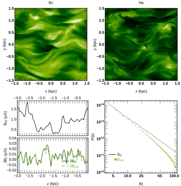
As a final illustration, figure 10 shows an implementation of the linear inversion on a more realistic reference field, B0
which is extracted from a magneto-hydrodynamical simulation (Kowal & Lazarian 2007), perturbed by a power-law fluctuation with a power spectrum ofα = 2 and a relative amplitude of 10−2
from a virtual data set of SNR=20. Note that for this more realistic illustration the electronic density neis not constant but extracted
from the same simulation. Both the shape of the correction and its power-spectrum are well recovered for this relative amplitude re-flecting that although non constant model and electronic density impair the conditionning, reconstructions remain possible.
5 CONCLUSION AND PERSPECTIVES
We investigated the problem of reconstructing the three-dimensional spatial structure of the magnetic field of a given simu-lated patch of our Galaxy, using multi-frequency polarized maps of
−1.5 −1.0 −0.5 0.0 0.5 1.0 1.5 −1.5 −1.0 −0.5 0.0 0.5 1.0 1.5 x (kpc) y (kpc) Bz −1.5 −1.0 −0.5 0.0 0.5 1.0 1.5 −1.5 −1.0 −0.5 0.0 0.5 1.0 1.5 x (kpc) y (kpc) Ne −3.0 −2.5 −2.0 −1.5 −1.0 −0.5 −0.02 −0.01 0.00 0.01 0.02 0.03 0.04 −3.0 −2.5 −2.0 −1.5 −1.0 −0.5 0.5 1.0 1.5 B0z ( µ G) δBin δBout z (kpc) δ Bz ( µ G) 10.0 20. 100.0 5. 50. 10+0 10+1 10+2 10+3 10+4 |k| P(k) Bin Bout
Figure 10. left top panel: map of a slice (of width0.047kpc) of input reference magnetic field, B0; right top panel: map of the same slice but for the known electronic densityne; left bottom panel: the input reference magnetic field, the input perturbation and the recovered one along a LOS. The perturbation field is a power-law fluctuation with a power spectrum ofα = 2 and a relative amplitude of 10−2from a virtual data set of SNR=20; right bottom panel: input and
recovered power spectra of the perturbation field.
the synchrotron emission at radio wavelengths.
When starting from a fair approximation of the magnetic field, we were able to obtain a good estimate of the underlying field by us-ing a linearized version of the inverse problem considered, up to a
643 grid size. The spectral analysis of the strictly linear problem
(with a constant reference field, and the simulated data obtained through a linearized model) allowed us to specify the best sam-pling strategy in electromagnetic frequency, and predict a spatially anisotropic distribution of posterior errors.
The best sampling strategy is in equal ∆λ2; it follows from the shape of(∂P/∂B0) along one LOS, which can be approximately
recast into a unitary Vandermond matrix when this particular sam-pling is used. The errors on the reconstructedBxandBy
compo-nents of the field are shown to be larger than the error on theBz
component. This anisotropy can be traced back to the shape of the
posterior covariance, and ultimately of the linearized model which is highly anisotropic, as only thez component of the field induces
Faraday rotation.
We considered in turn three more realistic cases: (i) a pseudo linear model (linear reconstruction of non-linearly simulated data), (ii) a varying reference model B0, and (iii) a varying reference
model B0and a (known) varying electronic density ne. We found
that for these reconstructions, the global conditioning of the mini-mum variance solution remained tractable. Finally, we investigated the case where the reference field is given by the outcome of a magneto-hydrodynamical simulation, and is perturbed by an additional fluctuating component of known power spectrum. We showed that even in this case the linear reconstruction quality is reasonable. This leads us to claim that a full non-linear reconstruc-tion, based on a Gauss-Newton sequence of linear sub-problems of
varying reference field, should be achievable.
Possible extensions of this work, beyond the scope of this paper, involve investigating systematically the degeneracies of the non-linear inversion. It would be worthwhile to construct specific estimators for the (possibly anisotropic) local power spectrum of the field (see e.g. Lazarian & Pogosyan 2006). Finally, from a mod-elling point of view, one of the main limitations of the present method is that we had to assume known thermal and relativistic electronic densities, in order to obtain a well posed inverse prob-lem from synchrotron emission data alone. However, we could in principle relax this assumption by adding extra data constraining the electronic densities (e.g. Hα data, see Haffner et al. 2003) or
emission measures of pulsars, and attempt a joint reconstruction of the magnetic field and the electronic densities. Any prior statisti-cal information (e.g. extracted from MHD simulations) of possible correlation between B andne could be used in this context.
An-other possibility would be to use the extra information given by the circular polarization of synchrotron emission (see Appendix C); this circular polarization, if negligible in the case of low energy sources (like our Galaxy), is measurable in the case of relativis-tic radio sources (see e.g. Jones & Odell 1977), and opens a way to constrain the electronic density together with the magnetic field structure of the source.
Acknowledgments
We thank Jean Heyvaerts, Martin Lemoine and Guy Pelletier for fruitful comments on the early stages of this work. Special thanks to Alex Lazarian for providing us with his interstellar magneto hy-drodynamics simulations.
References
Beck R., Brandenburg A., Moss D., Shukurov A., Sokoloff D., 1996, ARA&A, 34, 55
Beck R., Shukurov A., Sokoloff D., Wielebinski R., 2003, AAP , 411, 99
Burn B. J., 1966, MNRAS, 133, 67
Cao Z., Zhong Dai B., Yang J. P., Zhang L., 2006, ArXiv Astro-physics e-prints
Celledoni E., Owren B., 2001
Cordova A., Gautschi W., Ruscheweyh S., 1990, Numerische Mathematik, 57, 577
Furlanetto S. R., Briggs F. H., 2004, New Astronomy Review, 48, 1039
Ginzburg V. L., Syrovatskii S. I., 1965, ARA&A, 3, 297
Golub G. H., Hansen P. C., O’Leary D. P., 2000, SIAM Journal on Matrix Analysis and Applications, 21, 185
Haffner L. M., Reynolds R. J., Tufte S. L., Madsen G. J., Jaehnig K. P., Percival J. W., 2003, ApJ Sup., 149, 405
Jones T. W., Odell S. L., 1977, ApJ, 214, 522
Kachelrieß M., Serpico P. D., Teshima M., 2007, Astroparticle Physics, 26, 378
Kowal G., Lazarian A., 2007, ApJ Let., 666, L69 Lazarian A., Pogosyan D., 2006, ApJ, 652, 1348 Nocedal J., 1980, Mathematics of Computation, 35, 773 Nocedal J., Wright S. J., 2006, Numerical Optimization, 2nd edn.
Springer Verlag
Pichon C., Thi´ebaut E., 1998, MNRAS, 301, 419 R¨ottgering H., 2003, New Astronomy Review, 47, 405
Ruzmaikin A. A., Sokolov D. D., Shukurov A. M., eds, 1988, Magnetic fields of galaxies Vol. 133 of Astrophysics and Space Science Library
Sazonov V. N., 1969, Soviet Astronomy, 13, 396 Shewchuk J. R., 1994
Sokoloff D. D., Bykov A. A., Shukurov A., Berkhuijsen E. M., Beck R., Poezd A. D., 1998, MNRAS, 299, 189
Tarantola A., 1987, Inverse Problem Theory. Elsevier
Thi´ebaut E., 2002, in Starck J.-L., Murtagh F. D., eds, Astronom-ical Data Analysis II Vol. 4847, Optimization issues in blind de-convolution algorithms. pp 174–183
Vogt C., Enßlin T. A., 2005, AAP , 434, 67
Wahba G., ed. 1990, Spline models for observational data
APPENDIX A: THE CASEγ = 3
Forγ = 3, equation (5) takes a particularly simple expression P = A Z 0 −∞ ν−1nr(z)(B2x(z) − B2y(z) + 2iBx(z)By(z)) × exp„ 2iKν2 Z0 z ( neBz)(z′′)dz′′ « dz , (A1)
while equation (8) simplifies to:
∂P (x⊥, ν) ∂Bx(r′) = δD(r − r ′ )2Ahν−1nr(r′)(Bx+ iBy)(r′) × exp 2iKhν2 X z′′ θH(z′′− z′)( neBz)(x′, y′, z′′) ! . (A2) Note that for this value ofγ the two derivatives with respect to the
transverse magnetic field are thus related:
∂P (x⊥, ν)
∂By(r′)
= i∂P (x⊥, ν) ∂Bx(r′)
. (A3)
APPENDIX B: SOLENOIDAL FIELDS WITH FIXED POWER SPECTRUM.
The generation of solenoidal (divergence free) fields with fixed power spectra up to the Nyquist frequency is a tricky problem. The field must obey the three following conditions:
(i) fixed power spectrum:P (k) ∝ k−α, (ii) free divergence:∇ · B ≡ 0 ⇔ k ·Bˆ≡ 0,
(iii) reality of the field: ˆBk= ˆB−k⋆.
Given conditions (i) and (ii), the field is best generated in Fourier space. Since the field is multi periodic and we may write
ˆ
B = ˆB⊥1e⊥1+ ˆB⊥2e⊥2, (B1)
where ek≡ k/|k|, e⊥1and e⊥2form a spherical basis in Fourier
space, while ˆB⊥,i, i=1,2 are the projection over that basis of the
Fourier componant of the field. The vectors e⊥1and e⊥2are
cho-sen in such a way that ek⊥1/2= −e−k⊥1/2. The spherical basis is
direct for k and indirect for−k. In this representation, conditions
(ii) and (iii) become,
ˆ
Bk⊥1/2= − ˆB−k⊥1/2⋆ , and Bˆkk= 0. (B2)
So, the first step is to generate two complex fields ˆB⊥1and ˆB⊥2
Next, consider the frequencies that have no conjugate, i.e. the fre-quencyki= 0 (constant) and ki= Ny(Nyquist frequency) where
the indexi represents the Cartesian coordinates. Let us define F1
as the set of these two particular values, i.e. F1 = [0, Ny], and
F2the set of all the other values, i.e. for a vector of dimensionN ,
F2= [−(N/2 − 1), −(N/2 − 2), ..., −1, 1, ...N/2 − 2, N/2 − 1].
When the three components of k belong toF1, the reality condition
of the field is merelyIm ˆB = 0. After putting this imaginary part
to0, the field can be projected into the Cartesian basis.
The difficulty arises when one or two components belong toF1. For
example, consider the frequency k= (kx, ky, kz) with kx ∈ F1,
kyandkz ∈ F2. In this case, condition (iii) become ˆBk= ˆB−˜k⋆
where ˜k = (kx, −ky, −kz) is the “opposite” of k. The problem
is that in this case, ek⊥1/2 6= −e−˜k⊥1/2and the above discussed
method can no longer apply. Fortunately, the combination of con-dition (ii) and ˆBk= ˆB−˜k⋆ leads to the following set:
k·Bˆ ≡ 0, and Bˆk
x = 0. (B3)
So, the trick is to put the faulty component to0 and to generate the
other two as previously but in 2D space. Now, if k2D= (ky, kz),
we generate ˆB = ˆB⊥2De⊥2D, where ek2D ≡ k2D/|k2D| and
e⊥2Dform a polar basis in Fourier space. As previously, the vectors e⊥2Dare chosen in such a way that ek2D⊥2D = −e−k2D⊥2D. In
this 2D representation, conditions (ii) and (iii) lead to:
ˆ
Bk2D⊥2D= − ˆB
⋆
−k2D⊥2D, and Bˆk2Dk2D= 0. (B4)
Here we have only one degree of freedom left, thus, for these fre-quencies, we must generate one complex field ˆB⊥2Dwith the
de-sired power spectrum, and then apply equation (B4). Whenkyor
kzbelongs toF1, a similar procedure applies.
In the last case, two component belong toF1. For example, k =
(kx, ky, kz) with kx ∈ F2,ky andkz ∈ F1. In this case,
condi-tion (iii) become ˆBk = ˆB−˜k⋆ where ˜k = (−kx, ky, kz) is the
“opposite” of k. Again, ek⊥1/2 6= −e−˜k⊥1/2and the
combina-tion of condicombina-tion (ii) and ˆBk = ˆB−˜k⋆ leads to equations (B3).
Consequently, the same procedure follows for these frequencies. After inverse Fourier transform, one can check that the field is real, solenoidal and with the right power spectrum up to the Nyquist fre-quency.
APPENDIX C: CIRCULAR POLARIZATION
Since the rotating term depends on the density field of thermal elec-tronsnein the medium, we cannot separate, with the Faraday
ro-tation only,nefromBz. One way to tackle this problem is to pick
up the next coupling term of the Stokes parameters in the (optically thin medium, strong rotativity limit) assumption that describes our medium. This next term is a factor of conversion between linear and circular polarization, that can be considered together with the syn-chrotron emissivity of circular polarization (Jones & Odell 1977). Following the notations of Sazonov (1969), we write the transfer equation of the polarization tensorIαβas follows:
dIαβ(z) dz = Eαβ(z)−i(Tασ(z)δβτ−δασT ∗ βτ(z))Iστ(z) , (C1) withIαβ= „ I + Q U + iV U − iV I − Q « , andEαβ(z) is an emissivity
term. In the assumption of a thin, strongly rotating medium, we can retain only the rotating terms (the Hermitian part) ofTαβ. Defining
T = „
h q + if q − if −h
«
we can show that the transfer equation
can be reexpressed in terms of the(Q, V, U ) “vector” as: d dz 2 4 Q V U 3 5= 2 4 EQ EV EU 3 5− 2 4 h f q 3 5× 2 4 Q V U 3 5. (C2)
The fact that this differential equation involves multiplication by a non-Abelian group element - in SO(3) - prevents us from writing a formal solution to the equation in terms of exponentials. However, since we are in the end working on a discretized mesh, we can still write a formal solution to the discrete problem in terms of (finite) sums of (finite) rotations products as we will see below. One impor-tant point to notice, linked to the tensor nature of equation C1, is the transformation law of these “vectors” under rotation of the co-ordinate axes in the plane perpendicular to the line of sight. In this respect, the vector(h, q, f ) behaves the same way as the vector (Q, V, U ), i.e. the (Q, U )and (h, f ) subvectors are rotated by 2ψ
when the coordinate axes are rotated byψ. In the case of a
homo-geneous medium, this allows Sazonov (1969) and Jones & Odell (1977) to choose the coordinate axes used to measureQ and U so
that theV Stokes parameter couples only to U (this is achieved
whenq is set to 0). In this reference frame, the projection of the
(constant) magnetic field is aligned with the second coordinate axis. In the case of a fluctuating magnetic field, such a scheme is not possible anymore, and we need to rotate the coupling coefficients (best expressed in the reference frame given by the local projec-tion of the magnetic field) in a common, constant, reference frame. Thus, in an inhomogeneous medium, the equation C2 in the com-mon reference frame takes the form:
d dz 2 4 Q V U 3 5= 2 4 EQcos(2ψ) EV −EQsin(2ψ) 3 5− 2 4 h cos(2ψ) f −h sin(2ψ) 3 5× 2 4 Q V U 3 5, (C3) where(Q, U, V ) are measured in the common reference frame, and
all other quantities are defined in the frame of the local magnetic field. In the applications we will consider in this paper, the rota-tion coefficients are dominated by the contriburota-tion of cold (thermal) electrons of the medium. In this context,(h, f ) take the following
form (Sazonov 1969): h = − q 4 eneB⊥2 4 π2m3 ec3ν3 , f = q 3 eneBk π m2 ec2ν2 .
It is interesting to note that both the frequency dependence, and the dependence on the magnetic field are different in the coupling terms. We note that C3 involves the multiplication of the Stokes “vector” by an element of a non-Abelian group (SO(3)), which pre-cludes finding a formal solution to this differential equation. How-ever, the linearity of the equation in the Stokes parameters, allows us to write a formal solution in the discretized case in terms of sums of products of rotations on the source terms. This equation is very similar to the rigid body type equations encountered in mechan-ics, with the (major) difference that it is linear. For simplicity, we will consider here a first-order discretization of the problem (i.e. we consider the different fields to be piecewise constant). The solution to the homogeneous Stokes transfer equation can be written as:
2 4 Q V U 3 5(z) = nz−1 Y i=0 exp(−∆zMi) 2 4 Q V U 3 5(z = 0) ,
whereMiis the skew-symmetric matrix corresponding to the
vec-tor(hicos(2ψi), fi, −hisin(2ψi)). This discretized solution
ab-sence of internal sources. It corresponds to the simplest possible case of integration of an equation on the SO(3) Lie Group (e.g. Celledoni & Owren 2001). By linearity, we can find the discrete solution to the transfer equation with sources (C3):
2 4 Q V U 3 5(z) = nz−1 X i=0 nz−1 Y j=i exp(−∆zMj) 2 4 EQicos(2ψi) EV i −EQisin(2ψi) 3 5,
withψ = arctan(Bx/By)6. This expression generalizes
equa-tion (6) and can be used to infer the Frechet derivatives of the po-larization field with respect to the magnetic field, as was done in section 2 from the integral solution. The source terms in the frame attached to the local transverse magnetic field read (Jones & Odell (1977)): EQ= C nrB γ+1 2 ⊥ ν −γ−12 , E V = −D nrBkB γ 2 ⊥ν −γ2 (C4) wherenris the distribution of high-energy electrons in the medium,
and C and D are constants that depend on the energy distribution of relativistic electrons. Note that in equation (C4),nris weighted
differently in the expressions ofEQandEV, hence we can in
prin-ciple disentangle B fromnr. Here different assumptions can be
made, namely assuming either thatnris related to the distribution
of thermal electronsne, or that it is constant, or that it is related
to the magnetic field pressure locally (see Beck et al. (2003) for a discussion of the different assumptions). Another possible path is to add external constraints on eitherne(coming for instance from
Hαobservations (see Haffner et al. 2003) or from dispersion
mea-surements of pulsars), or eventually on the relativistic electron dis-tributionnrwith diffuse gamma-ray measurements.