Model testing of an evacuation system in ice-covered water with waves

(1)

Publisher’s version / Version de l'éditeur:

Vous avez des questions? Nous pouvons vous aider. Pour communiquer directement avec un auteur, consultez la

première page de la revue dans laquelle son article a été publié afin de trouver ses coordonnées. Si vous n’arrivez

Questions? Contact the NRC Publications Archive team at

PublicationsArchive-ArchivesPublications@nrc-cnrc.gc.ca. If you wish to email the authors directly, please see the first page of the publication for their contact information.

https://publications-cnrc.canada.ca/fra/droits

L’accès à ce site Web et l’utilisation de son contenu sont assujettis aux conditions présentées dans le site LISEZ CES CONDITIONS ATTENTIVEMENT AVANT D’UTILISER CE SITE WEB.

Technical Report (National Research Council of Canada. Canadian Hydraulics

Centre), 2004-07

READ THESE TERMS AND CONDITIONS CAREFULLY BEFORE USING THIS WEBSITE.

https://nrc-publications.canada.ca/eng/copyright

NRC Publications Archive Record / Notice des Archives des publications du CNRC :

https://nrc-publications.canada.ca/eng/view/object/?id=a5bb1e7e-0c9f-4dc2-9541-ceff3840dd29 https://publications-cnrc.canada.ca/fra/voir/objet/?id=a5bb1e7e-0c9f-4dc2-9541-ceff3840dd29

For the publisher’s version, please access the DOI link below./ Pour consulter la version de l’éditeur, utilisez le lien DOI ci-dessous.

https://doi.org/10.4224/40000426

Access and use of this website and the material on it are subject to the Terms and Conditions set forth at

Model testing of an evacuation system in ice-covered water with waves

(2)

MODEL TESTING OF AN EVACUATION SYSTEM IN

ICE-COVERED WATER WITH WAVES

A. BARKER, A. SIMÕES RÉ, J. WALSH AND E. KENNEDY

CHC TECHNICAL REPORT

PERD/CHC Report 61-6

CHC-TR-025

(3)

(4)

MODEL TESTING OF AN EVACUATION SYSTEM IN

ICE-COVERED WATER WITH WAVES

A. Barker1, A. Simões Ré2, J. Walsh1 and E. Kennedy2 1_{Canadian Hydraulics Centre}

National Research Council of Canada Ottawa, ON K1A 0R6 Canada 2

Institute for Ocean Technology National Research Council of Canada St. John’s, NF A1B 3T5 Canada

CHC Technical Report PERD/CHC Report 61-6 CHC-TR-025

(5)

(6)

ABSTRACT

A series of laboratory testing programs have been carried out to study the navigability of a conventional lifeboat design in a variety of environmental conditions. The present test series investigated the combined effects of ice and waves on this lifeboat design. The model lifeboat was constructed at a scale of 1:13. The variables in the test program included ice concentration, wave period and launch direction. The lifeboat had to meet a pass/fail criterion, which depended on whether the vessel could make way in a given environmental condition. Overall, the lifeboat was able to make way in all cases when traveling with the wave direction. Traveling into the waves, however, the vessel rarely made head way except in very light ice conditions. Compared to a previous test series with ice but no waves, the lifeboat was able to travel through higher ice concentrations when waves were present, compared to when there were no waves (as long as the vessel was traveling with the waves). Additionally, the vessel had a number of major problems, including lifeboat navigational break-downs due to ice becoming jammed in the propellers, the vessel becoming beached upon ice floes and poor visibility with respect to navigation using the onboard window. The ice floe collisions that the vessel encountered were also severe. The results provide further insight into the viability of conventional evacuation lifeboat systems in ice-covered water conditions.

(7)

(8)

MODEL TESTING OF AN EVACUATION SYSTEM IN

ICE-COVERED WATER WITH WAVES

1. INTRODUCTION

The incorporation of escape-evacuation-rescue (EER) systems on offshore structures is obviously an important aspect of platform design. These systems need to take into account not only a wide range of possible hazards and structure design, but also a wide range of environmental conditions. Moreover, conventional lifeboats are often the primary means of evacuation from offshore structures. While these vessels may be satisfactory in open-water conditions, the question arises as to their capabilities in ice-covered water. In these situations, the lifeboat must be able to withstand potential conditions with higher loading and limited navigability, compared to open water.

Factors that will affect lifeboat performance in ice-covered water include ice concentration, thickness and strength, the prevalence of land-fast or pack ice conditions, the presence of waves and the physical features of the ice, such as ridging. In order to evaluate the effectiveness of an evacuation system, or a part thereof, these factors must be taken into account in the design and operation of an EER system (see, for example, Poplin et al., 1998a and 1998b; Wright et al., 2003).

The presence of both ice and waves surrounding an offshore platform could occur off of the Eastern coast of Canada (the Grand Banks region), where offshore development is presently occurring. In this region, pack ice could potentially surround an offshore platform, and certainly the wave climate in this region is known to be severe. There are additional implications that make the study of lifeboat performance in ice and waves important. In the event of an emergency with toxic fumes or smoke plumes, it could become necessary for a lifeboat to travel in a specific direction, for example, upwind of the compromised structure. However, upwind is often also updrift (that is, into the waves). For these reasons, it is important to investigate the manoeuvrability of a vessel in both ice and waves.

(11)

2. PROJECT OBJECTIVES AND SCOPE

The project objectives were a continuation and expansion of those of the previous test series (Simões Ré et al, 2003). In that series of tests, the performance of a conventional lifeboat in ice was investigated, with various ice concentrations, piece sizes, ice thicknesses and with two different power capabilities. The aim was to determine performance boundaries of the lifeboat in these varying conditions. In the present test series, the presence of two types of waves were added to some of the previous test configurations, to study the implications of waves on lifeboat performance in ice.

The test series was carried out at a scale factor of 1:13. Table 1 shows the scaling factors for a variety of the test properties. The characteristics that were varied in the present tests were the ice concentration, wave period and launch direction. The two primary ice concentrations that were investigated were chosen based on those concentrations in the previous test series where the lifeboat had both pass and fail results (8 or 7 tenths); that is, those concentrations where the lifeboat both did and did not travel a distance of 7.5 times the lifeboat length (75 m full-scale distance). These concentrations were chosen in order to determine whether the addition of waves to the ice “regime” would hinder or aid the lifeboat’s performance. The thickness of the ice sheet was nominally 50 mm. Additionally, a sheet of ice was grown where the concentration of ice was 5/10ths (and the thickness was 25 mm). This ice was used in order to test the equipment, but the results have been included here (see page 11 for details).

The wave parameters were determined for conditions without ice. The wave height was kept constant at 0.1 m (model scale) for all but one of the test configurations. The wave period, in model scale, was either a “storm” condition of 1.0 s or a “swell” condition of 1.6 s. These values were chosen for two reasons: they were representative of moderately extreme conditions in the Grand Banks region offshore Canada, and they were also at the limit of the capabilities of the wave machines in the ice tank.

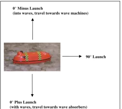
The tests primarily investigated two launch directions: the vessel facing into the waves and away from the waves (referred to as 0° Minus or 0° Plus launches respectively, i.e. 0° and 180° to the direction of travel of the waves). The launch direction was changed in order to study how well the vessel could make headway into the waves or how effectively it could be propelled when traveling with the waves. A few additional tests investigated the effects of launching the vessel at 90° to the direction of wave travel (that is, parallel to the wave trains).

The ice thickness investigated was the larger value used in the previous tests – nominally 50 mm in model scale. Piece size was randomly generated, in order to reflect a natural ice regime. The effects of additional power were not investigated in the present test program.

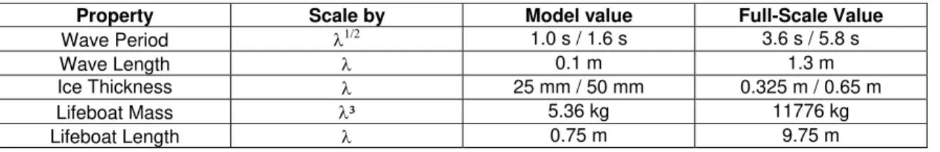
Table 1 Modelling Laws for the Physical Model Tests; λ = 13

Property Scale by Model value Full-Scale Value

Wave Period λ1/2 1.0 s / 1.6 s 3.6 s / 5.8 s

Wave Length λ 0.1 m 1.3 m

Ice Thickness λ 25 mm / 50 mm 0.325 m / 0.65 m

Lifeboat Mass λ³ 5.36 kg 11776 kg

(12)

3. TEST SET-UP

3.1 Test Facility

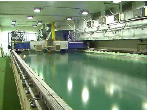
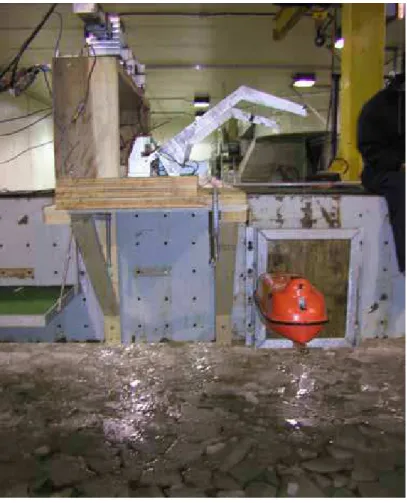
The tests were performed in the ice tank at the NRC Canadian Hydraulics Centre (CHC) in Ottawa (Pratte and Timco, 1981). Previous tests were held at the NRC Institute for Ocean Technology (IOT) (Simões Ré et al, 2003; Simões Ré et al, 2002), however the IOT ice tank is not able to accommodate a wave machine. The CHC tank, which is 21 m long by 7 m wide and 1.2 m deep, has a removable gate that facilitates access by a loader for moving the wave machines into the ice tank, and is housed in a large insulated room equipped with loading bay doors. The room can be cooled to an air temperature of -20°C. By varying the room's air temperature, ice sheets can be grown, tempered or melted. Spanning the ice tank is a carriage that can travel the length of the tank. The carriage is driven through two helical-cut rack and pinion gears, and is designed for loads up to 50 kN with a speed range from 3 to 650 mm/s. The evacuation system was mounted onto the main carriage. A small service carriage also spans the tank and this was used to mount wave gauges for sampling purposes. A photograph of the tank is shown in Figure 1.

Figure 1 Ice tank at the Canadian Hydraulics Centre.

3.2 Ice

3.2.1 Model Ice Characteristics

PG/AD model ice was used for this test series. This model ice is based on the EG/AD/S model ice developed at NRC in Ottawa (Timco 1986). PG/AD model ice represents well, on a reduced scale, the flexural strength, uni-axial compressive strength, confined compressive strength and failure envelope of sea ice. In addition, there is reasonable scaling of the strain modulus, fracture

(13)

toughness and density. The paper by Timco (1986) gives details of the mechanical properties of the model ice.

3.2.2 Ice Sheet Preparation

The thickness of the ice was adjusted by selecting an appropriate freezing time to produce the desired thickness. The strength of the ice can be adjusted by altering the time allowed for warming-up the ice. Two ice sheets were used for the test series, although the first sheet was initially intended to be used for testing the acquisition systems only. This test sheet had a thickness of 25 mm and a concentration of 5/10ths. For the second, and primary, ice sheet, growth was started using “wet-seeding” to nucleate the ice and produce uniform characteristics. The thickness of this ice sheet was 50 mm. This ice sheet was used for two full days of testing at 8/10ths and 7/10ths concentrations.

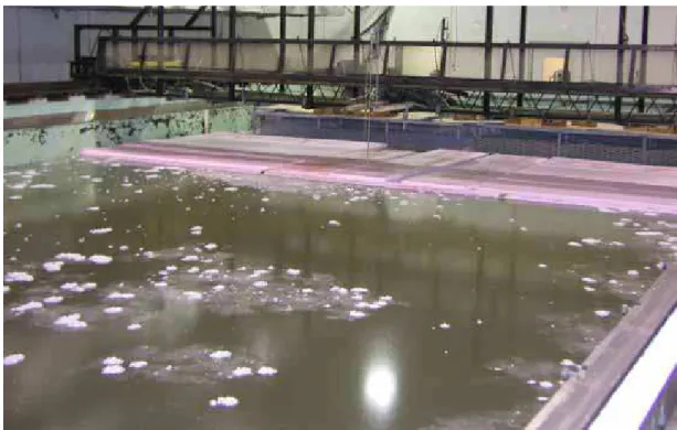
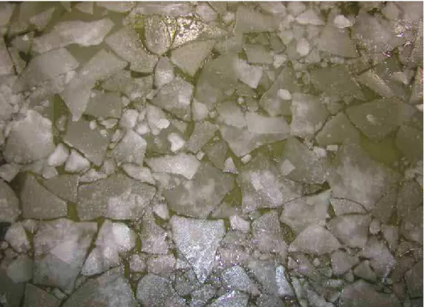
In order to achieve the desired concentration of ice in the tank, large sheets of rigid insulation were laid across the tank prior to freezing. At 8/10ths concentration, 14 sheets of insulation were required and these were laid on top of the water (Figure 2). On the morning of testing with the 50 mm thick ice, the temperature in the ice tank chamber was raised to hover around 2°C. The rigid sheets of insulation were removed, and staff randomly broke the ice using rakes and hoes in order to break up the ice sheet into floes. A photograph of the ice sheet after being broken into floes is shown in Figure 3. Figure 4 shows an example of an average piece size (approximately 20 cm). In order to achieve a lower concentration of ice on the second day of testing, wave action alone succeeded in lowering the concentration by the end of the first day of testing. However some additional ice was melted by raising the holding temperature of the ice tank overnight.

Figure 2 Preparing an ice sheet. Rigid insulation covers the water surface in order to control the concentration of ice in the tank.

(14)

Figure 3 Piece size distribution after breaking up an ice sheet.

Figure 4 Example piece size.

The effects of ice strength were not investigated, as the focus of the testing was the manoeuvrability of the TEMPSC in ice with a wave regime. However, the initial flexural strength of the ice was measured at the beginning of the second day of testing, prior to breaking up the ice into floes. Unlike the previous tests that investigated the effects of the TEMPSC in ice (but without waves), the strength could not be monitored throughout the testing, as there was no undisturbed ice that was suitable for performing flexural tests after the wave machines had been turned on. The initial flexural strength of the ice was 362 kPa, which was calculated by performing cantilever beam strength tests. The ice was initially significantly stronger then a correctly-scaled ice sheet. However, in this case the higher strength implies that floe splitting would not occur if the vessel hit a floe. By the end of each test day, approximately six or seven

(15)

3.3 Waves

In this test series, the objective was to examine some relatively extreme wave scenarios that may exist in the Grand Banks region offshore Canada.

3.3.1 Wave Generation

The water depth for all tests was 0.6 m. Wave generation was achieved using a computer-controlled portable wave machine. Sophisticated wave generation software permits the simulation of natural sea states as defined by parametric or measured spectra or by measured wave records.

3.3.2 Wave Absorption

In order to absorb wave energy in the ice tank, Progressive Wave Absorbers were placed at the opposite end of the ice tank from the wave machines. This patented type of wave absorber was developed at the CHC in the 1980’s, and is now used in several other offshore modelling basins and towing tanks around the world. The performance of the absorber depends on its length, and on the porosities of the constituent galvanized metal sheets. In larger model basins, the absorbers’ performance is quite good, with reflection coefficients in the order of 2-6%. In the ice tank, while no measurement of the absorption of the wave energy was made, it was not anticipated that a much larger level of reflection would be observed. More details about the performance of the wave absorbers can be found in Jamieson and Mansard (1987).

3.4 Evacuation System (TEMPSC Model)

Complete details of the lifeboat model may be found in Simões Ré et al (2002 and 2003). A summary of the model’s main features is presented here. The model had a scale of 1:13 and was representative of a 10 m long 80-person totally enclosed motor propelled survival craft (TEMPSC). In model scale, the vessel was approximately 0.75 m long, with a mass of 5.36 kg. The TEMPSC had a 32 mm four-bladed propeller, an active rudder, a wireless video camera, an electric motor and shaft, rechargeable batteries and a radio transmitter. The camera was mounted in the coxswain’s position. This provided a view that the vessel’s operator would have during an actual evacuation.

The evacuation system used to launch the TEMPSC was a conventional twin falls davit system, with dual motors and winches. The launch system was operated remotely. After the lifeboat was deployed from the davits, it was lowered to the water/ice surface and the falls were released from their hooks. The sail away phase was operated from within the ice tank, due to signal interference from the outer walls of the ice tank. At the end of each test, the lifeboat was driven to the edge of the tank, where it was physically removed, inspected, then reconnected to the davit system. A photograph of the model and its launching system are shown in Figure 5, while scale drawings of the TEMPSC are shown in Figure 6.

(16)

Figure 5 TEMPSC model with launching system

(17)

4. INSTRUMENTATION

The instrumentation that collected data during the test series was as follows: For the TEMPSC:

• Three accelerometers recording TEMPSC longitudinal, lateral and vertical accelerations • Three rate gyros monitoring roll, pitch and yaw

• Miniature load cell • Motor controller

• Electronic switch identifying davit release time • Payout sensor

• Sensor to monitor signal loss

• One TEMPSC-mounted video camera For the ice tank:

• Two wave probes

• Two overhead video cameras to track XY position of TEMSPC.

Note that only the wave probe and overhead video data were analysed for this study. All analog sensors were calibrated before the start of the experiments. Some of these systems are described in further detail below.

4.1 Wave Data Acquisition

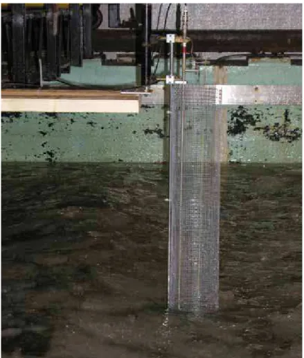
The wave height and periods used in this test series were based on un-damped values, that is, with no ice. Because of the dampening effect of pack ice on waves, an attempt was made to measure the wave heights that occurred during testing. Two capacitance-type wave probes were used to measure wave conditions near the end of the tank, close to the wave absorbers. The probes were mounted on the service carriage. Two photographs of the wave probe set-up are shown in Figure 7 and Figure 8. The wave probes were placed approximately 2.0 m apart.

The intent for this series was never to continually monitor the wave conditions, but to attempt to reproduce realistic wave climates. The wave probes were initially calibrated in the tank without ice, at room temperature, by moving them vertically in precisely measured increments while the water level was held constant. The probes typically feature calibration errors less than 0.5% over a 200 mm calibration range. They were then re-calibrated when the room temperature was dropped to near-freezing conditions. The calibrated wave machine sensors are presented in Appendix A. The first eight plots in Appendix D show the wave records recorded without ice. The probes were moved to sample two locations per probe, where position 1 is close to the wave machines and position 2 is close to the wave absorbers.

The probes operate by sensing the change in capacitance that occurs as a portion of the insulated wire becomes wetted. The output signal is directly proportional to the percentage of wire that is wetted, regardless of whether the wetting is continuous or intermittent (as with spray). These gauges have been used on many previous occasions and are known to exhibit highly linear and stable water level-to-voltage response. However, they have not been used in ice-covered water conditions. As such, protective coverings made of wire mesh were constructed in order to prevent ice from directly interacting with the probes. It was not always possible to prevent this occurrence however, and by the end of the test program, ice was routinely becoming stuck in the protective cages. The probes were sampled at a rate of 50 Hz. The data acquisition system was controlled using software (GEDAP) developed by CHC. The data from each test were stored in a single binary data file.

(18)

(19)

4.2 TEMPSC Data Acquisition

For the TEMPSC, the data acquisition was made through three systems: Shore based Daqbook 200 and radio telemetry receiver, on board A to D radio telemetry transmitter and wireless video. Two sampling frequencies were used. The Daqbook 200 data were filtered at 10Hz and sampled at 50Hz and the on board A to D transmitter signal was filtered at 50Hz and sampled at 250 Hz. The video data were sampled at a normal recording speed of 30 frames per second. The TEMPSC rudder angle was recorded by signal receiver duplication. A second servo, attached to a rotational variable differential transformer (RVDT) on shore, responded to the same signal being sent to the model. This was also recorded by the Daqbook 200 system. A detailed description of the TEMPSC data acquisition system may be found in Simões Ré et al (2003).

4.3 Co-ordinate System

4.3.1 Basin Co-ordinates

For the test basin, the co-ordinate system was right-handed. The positive X-axis is defined as up the tank towards the wave absorbers, the Y-axis is defined as the direction perpendicular to the carriage and the Z-axis is upwards. This is illustrated in Figure 9. Figure 10 is an illustration of the launch directions.

Service carriage Passive wave absorbers Melt pit Wave machines + X + Y + Z Launch platform Wave probes

Figure 9 Sketch of ice tank set-up and basin co-ordinate system

4.3.2 TEMPSC Co-ordinates

The TEMPSC had a fixed system, with the origin at the aft of the keel along the centre line. This right-handed coordinate system is fixed to the TEMPSC and moves with it. It defines the location of equipment in the TEMPSC, the location of the release mechanisms, the wireless camera position and the accelerometers. Further details about this system were provided in the previous study (Simões Ré et al, 2003). The motion pack was located close to the centre of gravity within the TEMPSC model.

4.4 Video

Two video cameras were mounted over the test area of the ice tank. The purpose of mounting the cameras in this manner was to use the resulting videos to track the x-y movement of the lifeboat.

(20)

In previous tests, the QUALISYS optical tracking system was used to track the x-y movement of the TEMPSC. However, this system was not available for the present test series, hence the use of the camera system. The cameras were spaced such that a total travel distance of approximately 7.5 boat-lengths was covered by the two cameras combined. However, the field of view of the cameras was such that the entire width of the ice tank could not be covered. If the lifeboat drifted or was propelled a wide distance off the centerline of the tank, the lifeboat could no longer be observed by the cameras and this portion of the lifeboat track would be lost. Some video data was also collected from a tripod-mounted camera. However this data is suitable for qualitative analysis only (whether the vessel met the pass/fail criterion), not x-y positioning.

The video camera located onboard the TEMPSC had, in previous tests, been used by the lifeboat operator to provide the same view as the TEMPSC coxswain. There were some concerns that the signal would be insufficient to operate the lifeboat from outside of the ice tank, where the video system was set up. Additionally, after the test ice sheet, it became apparent that the view was insufficient for navigating in waves and ice. As a result of these two concerns, the operator opted instead to operate the lifeboat from atop the main carriage in the ice tank, navigating by looking down on the lifeboat, rather than using the view from the on-board camera. This decision is discussed further in Section 7.

Figure 10 Illustration of launch directions

0° Plus Launch

(with waves, travel towards wave absorbers)

90° Launch 0° Minus Launch

(21)

5. TEST PROGRAM

5.1 Test Methodology

The test methodology was similar to the previous tests in ice without waves, and proceeded as follows:

• The test configuration was set according to the matrix.

• The davit twin fall lines were winched-up to the bulwark deck level. • The TEMPSC was attached to the davit twin-falls.

• The TEMPSC was winched-up to the proper launching height.

• The TEMPSC data acquisition was started, followed by the TEMPSC video. • The overhead video recording was started.

• The wave probe data acquisition was started.

• The wave machines were initiated with the appropriate drive signal.

• After a manual signal was received, the deployment started. Half way between the TEMPSC launching rest position and the water surface, the TEMPSC propulsion system was started remotely. The deployment start coincided with the start of the wave machines as much as possible.

• After splashdown, the davit releases were activated. The vessel operator exercised the rudder control remotely during the TEMPSC sail away to the safe zone.

• After the TEMPSC either reached the safe zone or it could not travel any further, the wave machines and other data acquisition systems were stopped.

• After completion of the test, the members of the project team started preparation for the next run. A path was cleared through the ice for the TEMPSC to travel to the edge of the tank, where it was lifted out of the tank and reconnected to the launch system.

• The ice in the tank was raked back across the tank to re-cover the water surface.

• The time between test runs was approximately 10 minutes when all events ran smoothly.

5.2 Test Matrix

The complete test matrix consisted of testing two ice sheets. A total of 40 tests were performed. Table 2 shows the tests that were the primary focus of the laboratory program. Tests not included in Table 2 are those that were performed with no power, with lower amplitude waves, in still water and with a launch direction of 90° to the incoming waves. Details of all of the tests are shown in Table 3. An explanation of the test names may be found in Appendix B. The initial ice sheet was used for testing purposes, to ensure that the data sampling and operational aspects were functioning correctly. That ice sheet was quite thin, and the concentration of ice in the tank was very low, approximately 5/10ths with a nominal thickness of 25 mm. The main ice sheet examined consisted of ice with either 8/10ths or 7/10ths concentration, and was approximately twice as thick as the initial sheet. As previously mentioned, the water depth for all tests was 0.6 m.

Initially, for the tests at 8/10ths concentration, each test was performed three times. However, it became apparent that the test results were going to be very similar for each trial. For the remaining tests at 7/10ths concentration, two tests per configuration were carried out. As the trials at 5/10ths concentration were for testing purposes, only one or two tests were performed.

(22)

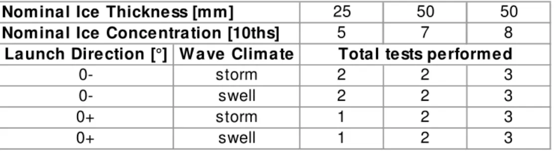
Table 2 Main test matrix

25 50 50

5 7 8

Launch Direction [°] Wave Climate

0- storm 2 2 3

0- swell 2 2 3

0+ storm 1 2 3

0+ swell 1 2 3

Nominal Ice Thickness [mm] Nominal Ice Concentration [10ths]

(23)

Table 3 Expanded details for the complete test matrix.

Test

# Test name Date

Nominal Ice Conc. [10ths] Launch Direction [°] Nominal Wave Height [m] Nominal Wave Period [s] 1 5_swell_0minus_001 12/09/03 5 0- 0.10 1.6 2 5_storm_0minus_001 12/09/03 5 0- 0.10 1.0 3 5_storm_0plus_001 12/09/03 5 0+ 0.10 1.0 4 5_swell_0plus_001 12/09/03 5 0+ 0.10 1.6 5 5_swell_0minus_002 12/09/03 5 0- 0.10 1.6 6 5_storm_0minus_002 12/09/03 5 0- 0.10 1.0 7 8_swell_0minus_001 12/10/03 8 0- 0.10 1.0 8 8_storm_0minus_001 12/10/03 8 0- 0.10 1.0 9 8_storm_0plus_001 12/10/03 8 0+ 0.10 1.0 10 8_swell_0plus_001 12/10/03 8 0+ 0.10 1.6 11 8_storm_0minus_002 12/10/03 8 0- 0.10 1.0 12 8_swell_0minus_002 12/10/03 8 0- 0.10 1.6 13 8_swell_0plus_002 12/10/03 8 0+ 0.10 1.6 14 8_storm_0plus_002 12/10/03 8 0+ 0.10 1.0 15 8_storm_0plus_003 12/10/03 8 0+ 0.10 1.0 16 8_swell_0plus_003 12/10/03 8 0+ 0.10 1.6 17 8_swell_0minus_003 12/10/03 8 0- 0.10 1.6 18 8_storm_0minus_003 12/10/03 8 0- 0.10 1.0 19 7_storm_0plus_001 12/11/03 7 0+ 0.10 1.0 20 7_swell_0plus_001 12/11/03 7 0+ 0.10 1.6 21 7_storm_0plus_002 12/11/03 7 0+ 0.10 1.0 22 7_swell_0plus_002 12/11/03 7 0+ 0.10 1.6 23 7_storm_0minus_001 12/11/03 7 0- 0.10 1.0 24 7_swell_0minus_001 12/11/03 7 0- 0.10 1.6 25 7_storm_0minus_002 12/11/03 7 0- 0.10 1.0 26 7_swell_0minus_002 12/11/03 7 0- 0.10 1.6 27 7_halfamp_storm_0minus_001 12/11/03 7 0- 0.05 1.0 28 7_halfamp_storm_0minus_002 12/11/03 7 0- 0.05 1.0 29 7_halfamp_storm_0minus_003 12/11/03 7 0- 0.05 1.0 30 7_nopower_swell_0plus_001 12/11/03 7 0+ 0.10 1.6 31 7_nopower_swell_0plus_002 12/11/03 7 0+ 0.10 1.6 32 7_T2p0_swell_0minus_001 12/11/03 7 0- 0.10 2.0 33 7_halftank_storm_0plus_001 12/11/03 7 0- 0.10 1.0 34 7_halftank_storm_0plus_002 12/11/03 7 0- 0.10 1.0 35 7_storm_90_001 12/11/03 7 90 0.10 1.0 36 7_storm_90_002 12/11/03 7 90 0.10 1.0 37 7_storm_90_003 12/11/03 7 90 0.10 1.0 38 7_storm_90and0plus_001 12/11/03 7 90 0.10 1.0 39 7_storm_90and0plus_002 12/11/03 7 90 0.10 1.0 40 7_stillwater_001 12/11/03 7 - 0.00 0.0

(24)

6. RESULTS

A complete summary of the results of the test program may be found in Appendix B. This appendix contains tables of data that summarize the pass/fail results for each test as well as the x-y plots of the vessel’s travel path. Appendix C shows some general photographs from the tests. As with the previous tests in ice, successful runs were defined as those for which the TEMPSC was able to launch and then sail away a set distance through the broken ice. Each test was given a pass or fail grade based on whether the boat made it through a distance of 75m (fullscale), or 7.5 boat lengths, from its launch point target. The TEMPSC was given a fail if it became lodged in heavy concentrations of ice in front of the wave absorbers, even though had it been able to travel a larger distance, it may have been a pass trial. Additionally, the TEMPSC was given a fail if it could not travel the set distance in its intended launch direction. For example, if the TEMPSC was supposed to be traveling into the waves, but ended up traveling with the waves, and successfully covering the 7.5 boat lengths, this was still considered a fail.

6.1 Video Analysis

The VHS videos were converted from analog video to digital video using an editing program called dpsReality. Before beginning the conversion from analog to digital, the VHS tapes had to be screened and logged. This made the process of converting easier. Any runs of poor video quality were not converted to digital videos. The video logs are found in Appendix D.

Once the videos had been screened and logged, the video was recorded in digital format and exported as .avi files. The video was not slowed down to convert it to full-scale time. These .avi files were then used in a program called VideoPoint Capture, allowing a specific number of frames to be selected for analysis. Typically 10-20 frames were determined to be sufficient for x-y plotting purposes. The digital video files were then compressed and saved. Finallx-y, the compressed files were opened in VideoPoint 2.5. The path of the vessel was then traced using the tracking capabilities of this program. For each frame, a point on the vessel had to be highlighted. Each point was represented by a set of x-y coordinates and the corresponding time. This data was exported to Excel and plotted as a representation of the path of the motion of the vessel.

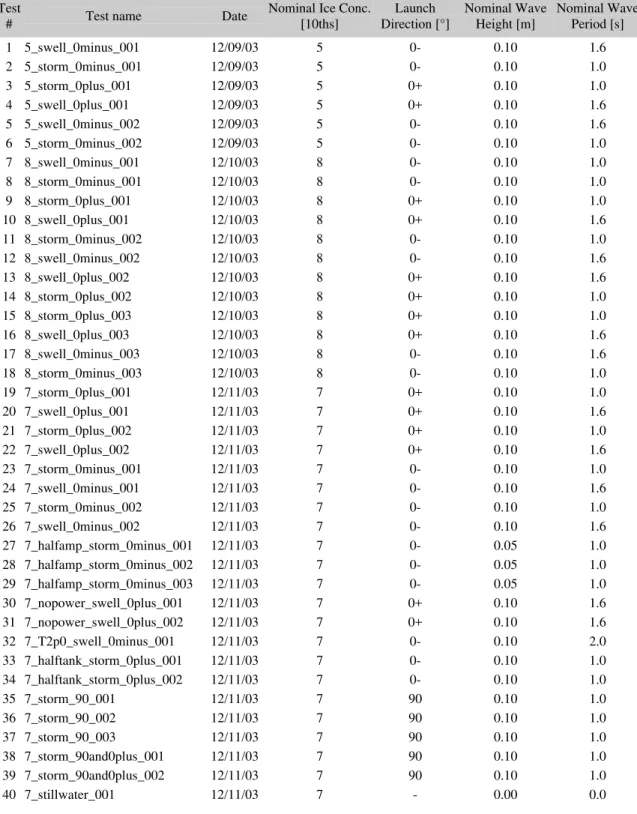
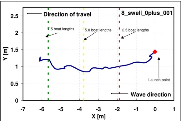
The data manipulation in Excel was straightforward. There was a correction that had to be made to the data for each test before plotting. The two overhead cameras were in a line, such that the vessel traveled from one camera’s field of view into the other. Although the initial video analysis for each camera is separate, the same initial reference point is used for each. This causes the two sets of data to be superimposed rather than continuous. To this end, a correction factor was calculated for camera B videos; a set value was added to the x- coordinates, to account for where the field of view of camera A ended and B should start. Also, the plotting order of the points from camera A and camera B depended on the direction of travel of the vessel. For motion in the positive direction (i.e. with the waves) data from camera B had to be listed before camera A and for a negative vessel direction (into the waves) data points for camera A were plotted before camera B. An example of a typical output plot is shown in Figure 11. The coloured, dotted lines indicate the location of 2.5, 5.0 and 7.5 boat lengths of travel distance. The red diamond indicates the launch location. Note that the direction of travel indicates the intended direction for the lifeboat, either into or with the waves, not the direction that the lifeboat may have ended up traveling.

(25)

8_swell_0plus_001

0

0.5

1

1.5

2

2.5 -7

-6

-5

-4

-3

-2

-1

0

1 X [m]

Y [

m

]

Wave direction

Direction of travel

Figure 11 Example x-y output from video analysis. Note that the direction of travel is the intended direction, which not necessarily the heading the vessel achieved.

Due to fuses blowing near the end of the test program, there were some runs that were not captured on overhead video. Additionally, some runs were not captured due to various errors. The tests that are missing overhead video data are:

• 5_storm_0minus_001 • 8_swell_0minus_002 • 8_swell_0plus_002 • 8_storm_0plus_002 • 8_storm_0plus_003 • 7_storm_0minus_001 • 7_swell_0minus_001 • 7_swell_0minus_002 • 7_halftank_storm_0minus_001 • 7_halftank_storm_0minus_002 • 7_storm_90_001 • 7_storm_90_002 • 7_storm_90_003 • 7_storm_90and0plus_001 • 7_storm_90and0plus_002 • 7_stillwater_001

While most tests had at least one overhead video, test 7_swell_0minus had none available for analysis. In most cases, however, video taken from the side of the tank was available to provide qualitative observations of the test, such as whether the pass/fail criterion was met. Figure 12 shows a photograph of the TEMPSC traveling through typical swell conditions, taken from the side of the tank.

7.5 boat lengths _{5.0 boat lengths} _{2.5 boat lengths}

(26)

Figure 12 Photograph taken from the side of the tank of TEMPSC traveling through swell waves.

6.2 Wave Probe Data Analysis

Plots of the wave probe data after it had been analysed can be found in Appendix E. Instances where the probes were not in the water are indicated in Table 4. An example of the output is shown in Figure 13, which includes the calculated significant wave height for each test (model scale). After the raw data were converted into binary files, basic statistical analysis was performed on the data. Zero-crossing and variance spectral density analysis were performed and a rectangular bandpass filter was applied to the signal. This filter removes all energy in the signal that occurs at frequencies below and above two specified frequencies. A Fourier transform of the input signal was computed and the rectangular bandpass filter was applied in the frequency domain. An inverse FFT was then used to obtain the filtered output signal.

As can be seen in Table 4, because of the ice routinely jamming in the protective cages surrounding the wave probes, the readings were unreliable, as expected. Where good readings were obtained, the storm wave heights were generally much lower than the 0.1 m nominal height, with values ranging from 0.01 m to 0.04 m. The swell readings, by contrast, were much higher than the nominal wave height, often almost three times as large. This could be due to the generation of standing waves in the ice tank under swell conditions. Table 5 illustrates the differences between the average maximum wave heights for conditions without and with ice. Once again, these results were not surprising.

(27)

Table 4 Wave probe analysis results. The frozen comment indicates that it was unclear whether the wave probe was correctly reading the wave heights, due to the possibility of ice

freezing onto the sensor.

Test name Nominal Wave Height [m] Nominal Wave Period [s] P1 in water? P2 in water? Hmo P1 (m) Hmo P2 (m) 5_swell_0minus_001 0.10 1.6 no no 5_storm_0minus_001 0.10 1.0 no no 5_storm_0plus_001 0.10 1.0 no no 5_swell_0plus_001 0.10 1.6 no no 5_swell_0minus_002 0.10 1.6 no no 5_storm_0minus_002 0.10 1.0 no no 8_swell_0minus_001 0.10 1.0 no no 8_storm_0minus_001 0.10 1.0 no no 8_storm_0plus_001 0.10 1.0 no no 8_swell_0plus_001 0.10 1.6 no no

8_storm_0minus_002 0.10 1.0 frozen? yes 0.001 0.010 8_swell_0minus_002 0.10 1.6 frozen? yes 0.001 0.337 8_swell_0plus_002 0.10 1.6 frozen? yes 0.001 0.361 8_storm_0plus_002 0.10 1.0 frozen? yes 0.001 0.007 8_storm_0plus_003 0.10 1.0 frozen? yes 0.001 0.004 8_swell_0plus_003 0.10 1.6 frozen? yes 0.001 0.342 8_swell_0minus_003 0.10 1.6 frozen? yes 0.001 0.349 8_storm_0minus_003 0.10 1.0 frozen? yes 0.002 0.011

7_storm_0plus_001 0.10 1.0 yes yes 0.023 0.022

7_swell_0plus_001 0.10 1.6 yes yes 0.162 0.351

7_storm_0plus_002 0.10 1.0 yes yes 0.032 0.017

7_swell_0plus_002 0.10 1.6 yes yes 0.165 0.308 7_storm_0minus_001 0.10 1.0 frozen? frozen? 0.004 0.002

7_swell_0minus_001 0.10 1.6 yes yes 0.162 0.300 7_storm_0minus_002 0.10 1.0 yes yes 0.038 0.006 7_swell_0minus_002 0.10 1.6 yes yes 0.131 0.239 7_halfamp_storm_0minus_001 0.05 1.0 no no

7_halfamp_storm_0minus_002 0.05 1.0 no no 7_halfamp_storm_0minus_003 0.05 1.0 no no

7_nopower_swell_0plus_001 0.10 1.6 yes yes 0.154 0.231 7_nopower_swell_0plus_002 0.10 1.6 yes no 0.194 7_T2p0_swell_0minus_001 0.10 2.0 yes no 0.164 7_halftank_storm_0plus_001 0.10 1.0 frozen? no 0.037 7_halftank_storm_0plus_002 0.10 1.0 frozen? no 0.015 7_storm_90_001 0.10 1.0 no no 7_storm_90_002 0.10 1.0 no no 7_storm_90_003 0.10 1.0 no no 7_storm_90and0plus_001 0.10 1.0 no no 7_storm_90and0plus_002 0.10 1.0 no no 7_stillwater_001 0.00 0.0 no no

(28)

Figure 13 Example of wave analysis output plot.

Table 5 Average maximum wave heights for various conditions in the ice tank

No ice 7/10s Concentration 8/10s Concentration

Average Hmax Storm 0.1066 0.0086 0.0014

(29)

7. DISCUSSION

7.1 Effect of Waves and Ice Combined

Table 6 shows the results for the main test matrix (those indicated in Table 2, page 13). In the table, an F indicates a fail while a P indicates a pass. These grades are preceded by the number of tests in that configuration that received that grade. It can be seen that generally the limiting factor to whether the TEMPSC passed or failed was the direction of travel, rather than the ice concentration. Results with an asterix (*) indicate that overhead video data was missing for one or more tests. Where available, video taken from the side of the tank was used to assess whether the vessel had a probable pass or fail.

It should be noted that unlike the previous test series in ice, where all tests of the same configuration received the same grade (i.e. all tests with small floes at 7/10ths concentration and 25 mm ice thickness passed), this was not the case in the present series. Results with an underscore (_) indicate that there were one or more tests where the TEMPSC became trapped the ice. This occurred during the testing program because the ice rafted up quickly at the end of the ice tank, limiting the amount of time the TEMPSC could travel through a relatively uniform concentration of ice. Not surprisingly, near the end of every test, the TEMPSC became trapped in what was essentially rafted (2-3 layers of ice), 10/10ths ice and could not move under its own power. This unfortunately resulted in a number of tests where the TEMPSC might have achieved a pass, had there been more room for the vessel to travel. This can be seen by comparing Table 6 with Table 7. In Table 7, the pass/fail criterion is changed to 5.0 boat lengths – note that this clearly illustrates the division between the trials where the TEMPSC successfully traversed the required distance and those where it did not. Figure 14 shows the TEMPSC trapped in ice at the end of a test.

Table 6 Results for the main test matrix; pass/fail criterion set at 7.5 boat-lengths.

Average Ice Thickness [mm] 24 47 45

Nominal Ice Concentration [10ths] 5 7 8

Launch Direction [°]

Wave Climate Grade [Pass or Fail]

0- storm 1F* 0P 2F* 0P 3F 0P 0- swell 2F 0P 2F* 0P 3F* 0P

0+ storm 1F 0P 1P 1F 3F* 0P

0+ swell 1P 0F 2P 0F 3P* 0F

_ indicates boat trapped in 9/10ths + ice (probably PASS otherwise) * missing overhead video analysis for one or more tests

Table 7 Results when pass/fail criterion is set at 5.0 boat-lengths.

Average Ice Thickness [mm] 24 47 45

Nominal Ice Concentration [10ths] 5 7 8

Launch Direction [°]

Wave Climate Grade [Pass or Fail]

0- storm 1P* 0F 2F* 0P 3F 0P 0- swell 2F 0P 2F* 0P 3F* 0P 0+ storm 1P 0F 2P 0F 3P* 0F 0+ swell 1P 0F 2P 0F 3P* 0F

(30)

Figure 14 Photograph during a test, showing the rafting and dense concentration of ice at the end of the tank.

In attempting to travel into the waves, the equivalent safe distance in the other direction was never achieved, as the boat could not make any headway due to the ice. Consequently the TEMPSC sometimes ended up achieving the safe distance in the opposite direction, as it drifted with the waves. As previously mentioned, this was still considered a fail situation. Figure 15 and Figure 16, for swell and storm tests respectively, illustrate the differences in travel path that occurred when the vessel traveled into or with the waves. Recall that the direction of travel is the intended direction of travel, which was not necessarily the direction that the vessel ended up traveling. 8_swell_0minus_003 0 0.5 1 1.5 2 2.5 -4 -3 -2 -1 0 1 2 3 X [m] Y [ m ] Wave direction

Direction of travel 8_swell_0plus_001

0 0.5 1 1.5 2 2.5 -7 -6 -5 -4 -3 -2 -1 0 1 X [m] Y [ m ] Wave direction Direction of travel

Time = 1 min 18 s Time = 51 s

(31)

8_storm_0minus_002 0 0.5 1 1.5 2 2.5 -2 -1 0 1 2 3 4 5 X [m] Y [ m ] Wave direction

Direction of travel _{8_storm_0plus_001}

0 0.5 1 1.5 2 2.5 -6 -5 -4 -3 -2 -1 0 1 X [m] Y [ m ] Wave direction Direction of travel

Time = 2 min 18 s Time = 1 min 49 s

Figure 16 Comparison of travel path in storm conditions.

The results of the extended test matrix are shown in Table 8. These tests were all performed with an ice concentration of 7/10ths. The most interesting results are those concerning the tests with no power and the still water test (without waves). For the latter test, the TEMPSC was unable to travel through the 7/10ths ice. This is as expected, given the results from the previous test series.

Table 8 Results of extended test matrix.

Average Ice Thickness [mm] 47

Nominal Ice Concentration [10ths] 7

Launch Direction [°] Wave Climate Condition Grade [Pass or Fail]

0- storm halfamp 3F 0+ swell no power 1P 0- swell T2P0 1F 0+ storm halftank -* 90 storm -* 90 storm 0+ 1F* 90 - still water 1F

Traveling with the waves, the TEMPSC almost always achieved an arbitrary safe distance from the structure. However, as shown during the test series with no power to the TEMPSC, this was achieved regardless of whether there was any power. While only one of the tests with no power appeared to pass, it should be noted that the overhead cameras did not document the launch of the TEMPSC. Therefore, it was likely that this test, like the other test with no power, was actually a pass. The duration may have taken slightly longer for the tests with no power, compared to those with power, but there was generally no question that the lifeboat would achieve the safe distance. This comparison is shown in Figure 17. As can be seen in these two plots, not only was the safe distance achieved in both tests, but the path through the ice was similar. The test time for the trial with power was approximately 30 s, while that without power was approximately 40 s.

As previously mentioned, navigability using the on-board video system was extremely difficult, if not futile, given the two wave conditions examined. It was almost impossible for the operator to try to pick a path through the floes, as the floes had changed position by the time the ice came into view again, riding down a crest. This is a real operational problem with current TEMPSC designs. In hindsight, it would perhaps have been worthwhile to navigate the TEMPSC using only the on-board video regardless, given that a TEMPSC operator at present would have no alternative. However, it did appear that the operator had little control over the path taken through

(32)

the ice, even with a full field of view looking down on the lifeboat. This is in contrast to the previous test series in ice with no waves, and with waves but no ice, where the operator was still able to use the on-board video system to manoeuvre the lifeboat, albeit with some difficulty, around ice floes or in line with a general heading. Also of interest was that during one test, the waves were such that the lifeboat became beached on some ice that was frozen onto the wave absorbers. The end result is shown in Figure 18. Subsequently, the wave machines were stopped before this type of event could reoccur, to avoid damage to the lifeboat.

7_swell_0plus_002 0 0.5 1 1.5 2 2.5 -6 -5 -4 -3 -2 -1 0 1 X [m] Y [ m ] Wave direction Direction of travel 7_nopower_swell_0plus_001 0 0.5 1 1.5 2 2.5 -6 -5 -4 -3 -2 -1 0 1 X [m] Y [ m ] Wave direction Direction of travel

Figure 17 Plots comparing a test (a) with power with the same test (b) without power. (b)

(33)

Figure 18 TEMPSC beached on ice ledge attached to wave absorbers.

7.2 Propeller Problems

Propeller problems occurred at least five times throughout the test series (out of the forty total runs). These failures generally happened when the TEMPSC was travelling with the waves, especially during the later stages of testing. At that point in the test series, the ice had been broken into smaller pieces, and was also weaker and “slushy”. The waves essentially pushed the ice into the propeller, which quickly became choked. Figure 19 shows the propeller jammed with ice on two different occasions. This led to a loss of rudder control almost immediately and in turn often led to problems with screw and tie wraps letting go, nuts backing off and similar problems with the inner mechanisms of the TEMPSC. A sketch of these problem locations is shown in Figure 20.

(34)

List of failure points (in no particular order)

A : The motor coupling set screw let go and the motor was slipping. B : The motor tie wrap let go and the tubing was slipping C : The stern shaft tie wrap let go and the tubing was slipping. D : The propeller holding nut backed off and the propeller was spilling E : The rudder set screw backed off causing excessive zero offset.

Drive Motor

B Motor tie wrap A Set screw on motor coupling Stern shaft Stern tube Propeller Nozzle

D Prop holding nut

tubing

C Stern shaft tie wrap

Rudder arm

E Rudder set screw

Rudder shaft Flat

Figure 20 Sketch showing the list of failure points due to ice jamming in the propeller.

7.3 Comparison with Previous Test Programs

The present test series demonstrated that the TEMPSC was able to travel through 7/10ths and 8/10ths ice with waves in the direction of travel, where in previous tests little or no headway was achieved at these concentrations. An example of this is shown in Figure 21. Although the TEMPSC did not achieve a pass for the present test series in the example shown here, it was still able to travel considerably further than the previous test series with ice and no waves. However, it is noted that this was only the case for tests where the TEMPSC direction of travel coincided with the wave direction.

However, when comparing the present tests with the previous test series with waves but no ice, a different picture emerges. In this comparison, shown in Figure 22, it can be seen that the ice hindered vessel performance compared to waves alone. In the previous test series, the TEMPSC was able to make headway into the waves, in Beaufort-scale strong breeze conditions (i.e. average full-scale wave height 1.95-2.93 m). In the present series, headway was only achieved into the waves at a low ice concentration, with thin ice. Even then, it was difficult for the TEMPSC to meet the pass criterion.

(35)

8_storm_0plus_001 0 0.5 1 1.5 2 2.5 -6 -5 -4 -3 -2 -1 0 1 X [m] Y [ m ] Wave direction Direction of travel

Figure 21 Comparison of travel distance in ice (a) with and (b) without waves (b)

(36)

8_storm_0minus_003 0 0.5 1 1.5 2 2.5 -2 -1 0 1 2 3 4 5 X [m] Y [ m ] Wave direction Direction of travel

Figure 22 Comparison of tests with waves and (a) without and (b) with ice

While the present test series did not investigate the effects of additional power on the lifeboat’s performance, it could be worthwhile to investigate this aspect of performance in upcoming tests. In the previous tests series in ice with no waves, an increase in power had little effect on the performance of the lifeboat. However, it is possible that this additional power in waves and ice could affect the lifeboat’s ability to make headway into waves in ice-covered waters. Where previously the lifeboat ended up drifting “downstream” with the waves for all but the lowest concentrations of ice, perhaps the lifeboat could make moderate headway, or at least be able to travel slightly parallel and into the waves, with some additional power. This could have repercussions for evacuation procedures, depending upon lifeboat placement on topsides facilities and the implications for successful evacuation away from a compromised offshore platform where it may be imperative to travel upwind of the structure.

(b) (a)

(37)

8. SUMMARY

A physical model test program was carried out in order to investigate the effect of lifeboat performance in pack ice and waves. The results indicated that contrary to expectations, the addition of waves to pack ice could enhance the performance of a lifeboat. With the addition of waves, the lifeboat was able to traverse larger ice concentrations compared to what it could pass through in a previous test program with pack ice but without waves. However, this was only achievable when the vessel travelled with the waves. It was observed that a pass condition (where the lifeboat cleared a set distance of 7.5 boat-lengths from the structure) when travelling with the waves could be achieved with or without power to the model vessel. The wave climates investigated in this study were such that the waves pushed the vessel along, past the pass criterion mark, regardless, when the vessel was traveling with the wave direction. While this appears on first inspection to be a benefit, there are negative implications to this if, for some reason, it was imperative that the vessel travel upwind of a compromised platform. As well, the vessel had little control over the path travelled through the floes.

Additionally, the addition of waves could also hinder performance. In a previous test program with waves but no ice, the lifeboat was able to make headway into waves, away from a platform location. With the addition of ice, the lifeboat in the present tests was unable to make headway into the waves at higher concentrations of ice.

Difficulties arose with the model as ice conditions deteriorated into weaker ice of small piece size. When traveling with the waves, ice often became jammed into the propeller. This caused a number of problems, most notably the lost of rudder control. It was also next-to-impossible to use the on-board video system to navigate the TEMPSC through the ice floes. Unlike previous test series where this was feasible, although difficult, in the present tests, the floes had changed position by the time they were within the field of view of the on-board video camera, after the vessel rode up and down a wave.

In Figure 23, the effects of vessel heading, ice concentration and wave climate are summarized. Upcoming physical model tests in this series will repeat the simple conditions investigated in the previous test series with ice but no waves. In the new tests, three different lifeboat hull designs at a 1:7 scale will be manoeuvred through different ice concentrations and thicknesses, measuring motions, ice mass impacts and loads. Additional tests with ice and waves will also be performed, with smaller waves than those that were used in the present series.

(38)

Figure 23 Summary of results

0° Plus Launch (with waves):

Pass achieved most of the time. Pass achieved without power to vessel. Vessel jammed in high concentrations of ice. Propeller jammed with ice pieces.

Able to traverse high (7-8 tenths) concentrations of ice. Quicker travel time with swell conditions.

Visual from on-board video not useful.

90° Launch:

Some headway made to the side. Pushed along with waves.

Visual from on-board video not useful.

0° Minus Launch (into waves):

Pass rarely achieved except in low ice concentration. Vessel overpowered by ice and waves.

False “Pass” almost achieved in opposite direction. Visual from on-board video not useful.

(39)

9. ACKNOWLEDGEMENTS

The financial support of the PERD Marine Transportation and Safety Committee is gratefully acknowledged.

The authors would also like to thank T. Ennis who helped with the instrumentation and set-up of the model, and to the CHC Facility technical staff (J.-P. Des Becquets, B. Gow, D. Pelletier) for helping to set up the experiments.

(40)

10. REFERENCES

Jamieson, W. and Mansard, E. (1987) An Efficient Upright Wave Absorber. Proc. ASCE Specialty Conference on Coastal Hydrodynamics, Newark, USA., pp. 124-139.

Poplin, J.P., Wang, A.T. and W. St. Lawrence, 1998a. Consideration for the Escape, Evacuation and Rescue from Offshore Platforms in Ice-Covered Waters. Proceedings of the International Conference on Marine Disasters: Forecast and Reduction, pp 329-337, Beijing, China.

Poplin, J.P., Wang, A.T. and W. St. Lawrence, 1998b. Escape, Evacuation and Rescue Systems for Offshore Installations in Ice-Covered Waters. Proceedings of the International Conference on Marine Disasters: Forecast and Reduction, pp 338-350, Beijing, China.

Pratte, B.D. and Timco, G.W. 1981. A New Model Basin for the Testing of Ice-Structure Interactions. Proceedings 6th International Conference on Port and Ocean Engineering under Arctic Conditions, Vol. II, pp 857-866, Quebec City, Canada.

Simões Ré, A., Veitch, B., Elliot, B. and Mulroney, S. (2003) Model Testing of An Evacuation System in Ice Covered Water, IMD/NRC Report TR-2003-03, 142 pp.

Simões Ré, A., Veitch, B., Sullivan, M., Pelley, D., and Colbourne, B. (2002) Systematic experimental evaluation of lifeboat evacuation performance in a range of environmental conditions – Phase I. IMD/NRC Report TR-2002-02.

Timco, G.W. (1986) EG/AD/S: A New Type of Model Ice for Refrigerated Towing Tanks. Cold Regions Science and Technology, Vol. 12, pp 175-195.

Wright, B.D., Timco, G.W., Dunderdale, P. and Smith, M. 2003. An Overview of Evacuation Systems for Structures in Ice-covered Waters. Proceedings 17th International Conference on Port and Ocean Engineering under Arctic Conditions, POAC'03, Vol. 2, pp 765-774, Trondheim, Norway.

(41)

(42)

(43)

(44)

(45)

(46)

DEFINITIONS 8_swell_0minus_002

8 concentration in tenths [8/10's]

swell wave climate [swell = 0.1 m wave height and 1.6 s period]

0minus launch angle [0° with respect to the waves = parallel launch] and direction lifeboat attempted to travel with respect to the waves [minus=into the waves]

(47)

Tests in red indicate no video available for analysis; tests in blue indicate only side-view video available for analysis.

Test Name Concentratio n (10ths) Wave Condition s Launch Directio n Pass [7.5 boat lengths ] Pass [5.0 boat lengths ]

5_storm_0minus_001 5 storm 0- N/A N/A

5_storm_0minus_002 5 storm 0- Fail Pass

5_swell_0minus_001 5 swell 0- Fail Fail

5_storm_0plus_001 5 storm 0+ Fail Pass

5_swell_0plus_001 5 swell 0+ Pass Pass

7_storm_0minus_001 7 storm 0- Fail Fail

7_storm_0minus_002 7 storm 0- Fail Fail

7_storm_0plus_001 7 storm 0+ Fail Pass 7_storm_0plus_002 7 storm 0+ Pass Pass

8_storm_0minus_001 8 storm 0- Fail Fail 8_storm_0minus_002 8 storm 0- Fail Fail 8_storm_0minus_003 8 storm 0- Fail Fail

7_halfamp_storm_0minus_00

1 7 storm 0- Fail Fail

2 7 storm 0- Fail Pass

3 7 storm 0- Fail Fail

7_nopower_swell_0plus_001 7 swell 0+ Pass Pass 7_nopower_swell_0plus_002 7 swell 0+ Fail Pass

7_T2p0_swell_0minus_001 7 swell 0- Fail Pass

7_halftank_storm_0plus_001 7 storm 0- N/A N/A

7_halftank_storm_0plus_002 7 storm 0- N/A N/A

7_storm_90_001 7 storm 90 N/A N/A

7_storm_90and0plus_001 7 storm 90 Fail Pass

7_storm_90and0plus_002 7 storm 90 N/A N/A

(48)

5_swell_0minus_001 0 0.5 1 1.5 2 2.5 -1 0 1 2 3 4 5 6 X [m] Y [ m ] Wave direction Direction of travel 5_storm_0plus_001 0 0.5 1 1.5 2 2.5 -6 -5 -4 -3 -2 -1 0 1 X [m] Y [ m ] Wave direction Direction of travel

(49)

5_swell_0plus_001 0 0.5 1 1.5 2 2.5 -6 -5 -4 -3 -2 -1 0 1 X [m] Y [ m ] Wave direction Direction of travel 5_swell_0minus_002 0 0.5 1 1.5 2 2.5 -1 0 1 2 3 4 5 6 X [m] Y [ m ] Wave direction Direction of travel

(50)

5_storm_0minus_002 0 0.5 1 1.5 2 2.5 -2 -1 0 1 2 3 4 5 X [m] Y [ m ] Wave direction Direction of travel 8_swell_0minus_001 0 0.5 1 1.5 2 2.5 -2 -1 0 1 2 3 4 5 X [m] Y [ m ] Wave direction Direction of travel

(51)

8_storm_0minus_001 0 0.5 1 1.5 2 2.5 -1 0 1 2 3 4 5 6 X [m] Y [ m ] Wave direction Direction of travel 8_storm_0plus_001 0 0.5 1 1.5 2 2.5 -6 -5 -4 -3 -2 -1 0 1 X [m] Y [ m ] Wave direction Direction of travel

(52)

8_swell_0plus_001 0 0.5 1 1.5 2 2.5 -7 -6 -5 -4 -3 -2 -1 0 1 X [m] Y [ m ] Wave direction Direction of travel 8_storm_0minus_002 0 0.5 1 1.5 2 2.5 -2 -1 0 1 2 3 4 5 X [m] Y [ m ] Wave direction Direction of travel

(53)

8_swell_0plus_003 0 0.5 1 1.5 2 2.5 -6 -5 -4 -3 -2 -1 0 1 X [m] Y [ m ] Wave direction Direction of travel 8_swell_0minus_003 0 0.5 1 1.5 2 2.5 -4 -3 -2 -1 0 1 2 3 X [m] Y [ m ] Wave direction Direction of travel

(54)

8_storm_0minus_003 0 0.5 1 1.5 2 2.5 -2 -1 0 1 2 3 4 5 X [m] Y [ m ] Wave direction Direction of travel 7_storm_0plus_001 0 0.5 1 1.5 2 2.5 -6 -5 -4 -3 -2 -1 0 1 X [m] Y [ m ] Wave direction Direction of travel

(55)

7_swell_0plus_001 0 0.5 1 1.5 2 2.5 -6 -5 -4 -3 -2 -1 0 1 X [m] Y [ m ] Wave direction Direction of travel 7_storm_0plus_002 0 0.5 1 1.5 2 2.5 -6 -5 -4 -3 -2 -1 0 1 X [m] Y [ m ] Wave direction Direction of travel

(56)

7_swell_0plus_002 0 0.5 1 1.5 2 2.5 -6 -5 -4 -3 -2 -1 0 1 X [m] Y [ m ] Wave direction Direction of travel 7_storm_0minus_002 0 0.5 1 1.5 2 2.5 -3 -2 -1 0 1 2 3 4 X [m] Y [ m ] Wave direction Direction of travel

(57)

7_halfamp_storm_0minus_001 0 0.5 1 1.5 2 2.5 -1 0 1 2 3 4 5 6 X [m] Y [ m ] Wave direction Direction of travel 7_halfamp_storm_0minus_002 0 0.5 1 1.5 2 2.5 -1 0 1 2 3 4 5 6 X [m] Y [ m ] Wave direction Direction of travel

(58)

7_halfamp_storm_0minus_003 0 0.5 1 1.5 2 2.5 -1 0 1 2 3 4 5 6 X [m] Y [ m ] Wave direction Direction of travel 7_nopower_swell_0plus_001 0 0.5 1 1.5 2 2.5 -6 -5 -4 -3 -2 -1 0 1 X [m] Y [ m ] Wave direction Direction of travel

(59)

7_nopower_swell_0plus_002 0 0.5 1 1.5 2 2.5 -6 -5 -4 -3 -2 -1 0 1 X [m] Y [ m ] Wave direction Direction of travel 7_T2p0_swell_0minus_001 0 0.5 1 1.5 2 2.5 -2 -1 0 1 2 3 4 5 X [m] Y [ m ] Wave direction Direction of travel

(60)

APPENDIX C VIDEO LOG

(61)

VIDEO LOG

Test 1: 5_swell_0minus_001

Vessel was pushed back by the waves at first but made some headway into the waves. Vessel reached 2.5 boat lengths.

Test 2: 5_storm_0minus_001 No video available.

Test 3: 5_storm_0plus_001

The launch is not in field of view. Vessel pushed (helped along) by waves. Vessel reached 5.0 boat lengths.

Test 4: 5_swell_0plus_001

Vessel made headway into the waves and travelled far. Propeller failure noted. Vessel reached 2.5 boat lengths.

Test 6: 5_storm_0minus_002

Vessel was pushed back by the waves at first but then made headway into the waves. Vessel reached 5.0 boat lengths.

Vessel was pushed back by the waves. Could not make headway into the waves. Vessel did not reach 2.5 boat lengths.

Vessel gets stuck in ice. Test abandoned after approximately 3.5 minutes. Vessel did not reach 2.5 boat lengths.

Test 9: 8_storm_0plus_001

Test 10: 8_swell_0plus_001

Vessel was pushed back by the waves. Could not make headway into the waves. Vessel did not reach 2.5 boat lengths.

Model testing of an evacuation system in ice-covered water with waves

Publisher’s version / Version de l'éditeur:

Technical Report (National Research Council of Canada. Canadian Hydraulics

Centre), 2004-07

Model testing of an evacuation system in ice-covered water with waves

MODEL TESTING OF AN EVACUATION SYSTEM IN

ICE-COVERED WATER WITH WAVES

A. BARKER, A. SIMÕES RÉ, J. WALSH AND E. KENNEDY

CHC TECHNICAL REPORT

PERD/CHC Report 61-6

CHC-TR-025

MODEL TESTING OF AN EVACUATION SYSTEM IN

ICE-COVERED WATER WITH WAVES

ABSTRACT

TABLE OF CONTENTS

MODEL TESTING OF AN EVACUATION SYSTEM IN

ICE-COVERED WATER WITH WAVES

1. INTRODUCTION

2. PROJECT OBJECTIVES AND SCOPE

3. TEST SET-UP

4. INSTRUMENTATION

5. TEST PROGRAM

6. RESULTS

8_swell_0plus_001

0

0.5

1

1.5

2

2.5

-7

-6

-5

-4

-3

-2

-1

0

1

X [m]

Y [

m

]

Wave direction

Direction of travel

7. DISCUSSION

8. SUMMARY

9. ACKNOWLEDGEMENTS

10. REFERENCES

APPENDIX C VIDEO LOG