HAL Id: hal-02174445
https://hal.inria.fr/hal-02174445
Submitted on 5 Jul 2019
HAL is a multi-disciplinary open access
archive for the deposit and dissemination of
sci-entific research documents, whether they are
pub-lished or not. The documents may come from
teaching and research institutions in France or
abroad, or from public or private research centers.
L’archive ouverte pluridisciplinaire HAL, est
destinée au dépôt et à la diffusion de documents
scientifiques de niveau recherche, publiés ou non,
émanant des établissements d’enseignement et de
recherche français ou étrangers, des laboratoires
publics ou privés.
Adaptive Caching for Data-Intensive Scientific
Workflows in the Cloud
Gaëtan Heidsieck, Daniel de Oliveira, Esther Pacitti, Christophe Pradal,
Francois Tardieu, Patrick Valduriez
To cite this version:
Gaëtan Heidsieck, Daniel de Oliveira, Esther Pacitti, Christophe Pradal, Francois Tardieu, et al..
Adaptive Caching for Data-Intensive Scientific Workflows in the Cloud. DEXA 2019 - 30th
Interna-tional Conference on Database and Expert Systems Applications, Aug 2019, Linz, Austria. pp.452-466,
�10.1007/978-3-030-27618-8_33�. �hal-02174445�
Workflows in the Cloud
Ga¨etan Heidsieck1[0000−0003−2577−4275], Daniel de
Oliveira4[0000−0001−9346−7651], Esther Pacitti1[0000−0003−1370−9943], Christophe
Pradal1,2[0000−0002−2555−761X], Fran¸cois Tardieu3[0000−0002−7287−0094], and
Patrick Valduriez1[0000−0001−6506−7538]
1
Inria & LIRMM, Univ. Montpellier, France
2
CIRAD & AGAP, Montpellier SupAgro, France
3 INRA & LEPSE, Montpellier SupAgro, France 4
Institute of Computing, UFF, Brazil
Abstract. Many scientific experiments are now carried on using scien-tific workflows, which are becoming more and more data-intensive and complex. We consider the efficient execution of such workflows in the cloud. Since it is common for workflow users to reuse other workflows or data generated by other workflows, a promising approach for efficient workflow execution is to cache intermediate data and exploit it to avoid task re-execution. In this paper, we propose an adaptive caching solu-tion for data-intensive workflows in the cloud. Our solusolu-tion is based on a new scientific workflow management architecture that automatically manages the storage and reuse of intermediate data and adapts to the variations in task execution times and output data size. We evaluated our solution by implementing it in the OpenAlea system and performing extensive experiments on real data with a data-intensive application in plant phenotyping. The results show that adaptive caching can yield ma-jor performance gains, e.g., up to 120.16% with 6 workflow re-executions. Keywords: Adaptive Caching · Scientific Workflow · Cloud · Workflow Execution.
1
Introduction
In many scientific domains, e.g., bio-science [8], complex experiments typically require many processing or analysis steps over huge quantities of data. They can be represented as scientific workflows (SWfs), which facilitate the modeling, management and execution of computational activities linked by data dependen-cies. As the size of the data processed and the complexity of the computation keep increasing, these SWfs become data-intensive [8], thus requiring execution in a high-performance distributed and parallel environment, e.g. a large-scale virtual cluster in the cloud.
Most Scientific Workflow Management Systems (SWfMSs) can now execute SWfs in the cloud [12]. Some examples of such SWfMS are Swift/T, Pegasus,
SciCumulus, Kepler and OpenAlea, the latter being widely used in plant science for simulation and analysis.
It is common for workflow users to reuse other workflows or data gener-ated by other workflows. Reusing and re-purposing workflows allow for the user to develop new analyses faster [7]. Furthermore, a user may need to execute a workflow many times with different sets of parameters and input data to ana-lyze the impact of some experimental step, represented as a workflow fragment, i.e. a subset of the workflow activities and dependencies. In both cases, some fragments of the workflow will be executed many times, which can be highly re-source consuming and unnecessary long. Workflow re-execution can be avoided by storing the intermediate results of these workflow fragments and reuse them in later executions.
In OpenAlea, this is provided by a lazy evaluation technique, i.e. the in-termediate data is simply kept in memory after the execution of a workflow. This allows for a user to visualize and analyze all the activities of a workflow without any re-computation, even with some parameter changes. Although lazy evaluation represents a step forward, it has some limitations, e.g. it does not scale in distributed environments and requires much memory if the workflow is data-intensive.
In a single user perspective, the reuse of the previous results can be done by storing the relevant outputs of intermediate activities (intermediate data) within the workflow. This requires the user to manually manage the caching of the results that she wants to reuse, which can be difficult as she needs to be aware of the data size, execution time of each task, i.e. the instantiation of an activity during the execution of a workflow, or other factors that could allow deciding which data is the best to store.
A complementary, promising approach is to reuse intermediate data pro-duced by multiple executions of the same or different workflows. Some SWfMSs support the reuse of intermediate data, yet with some limitations. VisTrails [4] automatically makes the intermediate data persistent with the workflow defini-tion. With a plugin [20], VisTrails allows SWf execution in HPC environments, but does not benefit from reusing intermediate data. Kepler [2] manages a per-sistent cache of intermediate data in the cloud, but does not take data transfers from remote servers into account. There is also a trade-off between the cost of re-executing tasks versus storing intermediate data that is not trivial [1,6]. Yuan et al. [18] propose an algorithm based on the ratio between re-computation cost and storage cost at the task level. The algorithm is improved in [19] to take into account workflow fragments. Both algorithms are used before the execution of the workflow, using the provenance data of the intermediate datasets. However, this approach is static and cannot deal with variations in tasks’ execution times. In data intensive SWf, such variations can be very important depending on the input data, e.g., data compression tasks can be short or long depending on the data itself, regardless of size.
In this paper, we propose an adaptive caching solution for efficient execution of data-intensive workflows in the cloud. By adapting to the variations in tasks’
execution times, our solution can maximize the reuse of intermediate data pro-duced by workflows from multiple users. Our solution is based on a new SWfMS architecture that automatically manages the storage and reuse of intermediate data. Cache management is involved during two main steps: SWf preprocess-ing, to remove all fragments of the workflow that do not need to be executed; and cache provisioning, to decide at runtime which intermediate data should be cached. We propose an adaptive cache provisioning algorithm that deals with the variations in task execution times and output data. We evaluated our solution by implementing it in OpenAlea and performing extensive experiments on real data with a complex data-intensive application in plant phenotyping.
This paper is organized as follows. Section 2 presents our real use case in plant phenotyping. Section 3 introduces our SWfMS architecture in the cloud. Section 4 describes our cache algorithm. Section 5 gives our experimental evaluation. Finally, Section 6 concludes.
2
Use Case in Plant Phenotyping
In this section, we introduce in more details a real SWf use case in plant pheno-typing that will serve as motivation for the work and basis for the experimental evaluation.
In the last decade, high-throughput phenotyping platforms have emerged to allow for the acquisition of quantitative data on thousands of plants in well-controlled environmental conditions. These platforms produce huge quantities of heterogeneous data (images, environmental conditions and sensor outputs) and generate complex variables with in-silico data analyses. For instance, the seven facilities of the French Phenome project (https://www.phenome-emphasis.fr/ phenome_eng/) produce each year 200 Terabytes of data, which are heteroge-neous, multiscale and originate from different sites. Analyzing automatically and efficiently such massive datasets is an open, yet important, problem for biologists [17].
Computational infrastructures have been developed for processing plant phe-notyping datasets in distributed environments [14], where complex phephe-notyping analyses are expressed as SWfs. Such analyses can be represented, managed and shared in an efficient way, where compute- and data-based activities are linked by dependencies [5].
One scientific challenge in phenomics, i.e., the systematic study of pheno-types, is to analyze and reconstruct automatically the geometry and topology of thousands of plants in various conditions observed from various sensors [16]. For this purpose, we developped the OpenAlea Phenomenal software package [3]. Phenomenal provides fully automatic workflows dedicated to 3D reconstruction, segmentation and tracking of plant organs, and light interception to estimate plant biomass in various scenarios of climatic change [15].
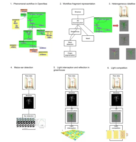
Phenomenal is continuously evolving with new state-of-the-art methods that are added, thus yielding new biological insights (see Figure 1). A typical work-flow is shown in Figure 1.1. It is composed of different fragments, i.e., reusable
Skeletonize Mesh 3D reconstruction Binarize Stem detection Organ segmentation
1. Phenomenal workflow in OpenAlea 2. Workflow fragment representation 3. Heterogeneous dataflow
4. Maize ear detection
Ear detection Binarize Raw data
5. Light interception and reflection in greenhouse 3D reconstruction Binarize Raw data Light interception 6. Light competition 3D reconstruction Binarize Raw data Light competition
Fig. 1: Use Cases in Plant Phenotyping. 1) The Phenomenal workflow in Ope-nAlea’s visual programming environment. The different colors represent different workflow fragments. 2) A conceptual view of the same workflow. 3) Raw and in-termediate data such as RGB images, 3D plant volumes, skeleton, and mesh. 4-5-6) Three different SWfs that reuse the same workflow fragments to address different scientific questions.
sub-workflows. In Figure 1.2, the different fragments are for binarization, 3D reconstruction, skeletonization, stem detection, organ segmentation and mesh generation. Other fragments such as greenhouse or field reconstruction, or sim-ulation of light interception, can be reused.
Based on these different workflow fragments, different users can conduct dif-ferent biological analyses using the same datasets. The SWf shown in Figure 1.4 reuses the Binarize fragment to predict the flowering time in maize. In Figure 1.5, the same Binarize fragment is reused and the 3D reconstruction fragment is added to reconstruct the volume of the 1,680 plants in 3D. Finally, in the SWf shown in Figure 1.6, the previous SWf is reused, but with different parameters to study the environmental versus genetic influence of biomass accumulation.
These three studies have in common both the plant species (in our case maize plants) and share some workflow fragments. At least, scientists want to compare their results on previous datasets and extend the existing workflow with their own developed actors or fragments. To save both time and resources, they want to reuse the intermediate results that have already been computed rather than recompute them from scratch.
The Phenoarch platform is one of the Phenome nodes in Montpellier. It has a capacity of 1,680 plants with a controlled environment (e.g., temperature, humidity, irrigation) and automatic imaging through time. The total size of the raw image dataset for one experiment is 11 Terabytes.
Currently, processing a full experiment with the phenomenal workflow on local computational resources would take more than one month, while scientists require this to be done over the night (12 hours). Furthermore, they need to restart an analysis by modifying parameters, fix errors in the analysis or extend it by adding new processing activities. Thus, we need to use more computational resources in the cloud including both large data storage that can be shared by multiple users.
3
Cloud SWfMS Architecture
In this section, we present our SWfMS architecture that integrates caching and reuse of intermediate data in the cloud. We motivate our design decisions and describe our architecture in two ways: first, in terms of functional layers (see Figure 2), which shows the different functions and components; then, in terms of nodes and components (see Figure 3), which are involved in the processing of SWfs.
Our architecture capitalizes on the latest advances in distributed and parallel computing to offer performance and scalability [13]. We consider a distributed architecture with on premise servers, where raw data is produced (e.g., by a phenotyping experimental platform in our use case), and a cloud site, where the SWf is executed. The cloud site (data center) is a shared-nothing cluster, i.e. a cluster of server machines, each with processor, memory and disk. We choose shared-nothing as it is the most scalable architecture for big data analysis.
In the cloud, metadata management has a critical impact on the efficiency of SWf scheduling as it provides a global view of data location, e.g. at which nodes some raw data is stored, and enables task tracking during execution [9]. We organize the metadata in three repositories: catalog, provenance database and cache index. The catalog contains all information about users (access rights, etc.), raw data location and SWfs (code libraries, application code). The prove-nance database captures all information about SWf execution. The cache index contains information about tasks and intermediate data produced, as well as the location of files that store the intermediate data. Thus, the cache index itself is small (only file references) and the cached data can be managed using the under-lying file system. A good solution for implementing these metadata repositories is a modern key-value store, such as Cassandra (https://cassandra.apache. org), which provides efficient key-based access, scalability and fault-tolerance through replication in a shared-nothing cluster.
The raw data (files) are intially produced at some servers, e.g. in our use case, at the phenotyping platform and get transferred to the cloud site. The cache data (files) are produced at the cloud site after SWf execution. A good solution to store these files in a cluster is a distributed file system like Lustre (http://lustre.org) which is used a lot in HPC as it scales to high numbers of files.
SWf manager (activity execution) SWf manager (activity execution)
Catalog ProvDB Cache index Catalog ProvDB Cache index
SWf data manager (files, data transfer, …) SWf data manager (files, data transfer, …)
Scheduler Cache Manager Task Manager Scheduler Cache Manager Task Manager
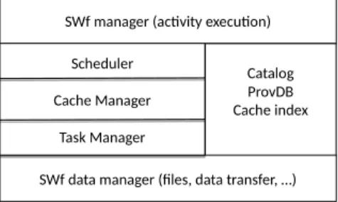
Fig. 2: SWfMS Functional Architecture
Figure 2 extends the SWfMS architecture proposed in [10], which distin-guishes various layers, to support intermediate data caching. The SWf manager is the component that the user clients interact with to develop, share and ex-ecute worksflows, using the metadata (catalog, provenance database and cache index). It determines the workflow activities that need to be executed, and gen-erates the associated tasks for the scheduler. It also uses the cache index for SWf preprocessing to identify the intermediate data to reuse and the tasks that need not be re-executed.
The scheduler exploits the catalog and provenance database to decide which tasks should be scheduled to cloud sites. The task manager controls task execu-tion and uses the cache manager to decide whether the task’s output data should
be placed in the cache. The cache manager implements the adaptive cache pro-visioning algorithm described in Section 4. The SWf data manager deals with data storage, using a distributed file system.
Figure 3. SWfMS Technical Architecture
Cloud site Cat Cat Prov DB Prov DB Cache index Cache index Master Node (SWf mgr, schedulers) Standby Master Node Server Server Data Node (SWf data mgr) Compute Node (SWf task mgr) Data
Data (SWf data mgr)Data Node Compute Node (SWf task mgr) Data Data Raw data Raw data Server Server Raw data Raw data
Fig. 3: SWfMS Technical Architecture
Figure 3 shows how these components are involved in SWf processing, using the traditional master-worker model. There are three kinds of nodes, master, compute and data nodes, which are all mapped to cluster nodes at configuration time, e.g. using a cluster manager like Yarn ( http://hadoop.apache.org). The master node includes the SWf manager, scheduler and cache manager, and deals with the metadata. The master node is lightly loaded as most of the work of serving clients is done by the compute and data nodes (or worker nodes), which perform task management and execution, and data management, respectively. So, it is not a bootleneck. However, to avoid any single point of failure, there is a standby master node that can perform failover upon the master node’s failure. Let us now illustrate briefly how SWf processing works. User clients con-nect to the cloud site’s master node. SWf execution is controlled by the master node, which identifies, using the SWf manager, which activities in the fragment can take advantage of cached data, thus avoiding task execution. The scheduler schedules the corresponding tasks that need to be processed on compute nodes which in turn will rely on data nodes for data access. It also adds the transfers of raw data from remote servers that are needed for executing the SWf. For each task, the task manager decides whether the task’s output data should be placed in the cache taking into account storage costs, data size, network costs. When a task terminates, the compute node sends to its master the task’s execution information to be added in the provenance database. Then, the master node updates the provenance database and may trigger subsequent tasks
4
Cache Management
We start by introducing some terms and concepts. A SWf W (A, D) is the abstract representation of a directed acyclic graph (DAG) of computational ac-tivities A and their data dependencies D. There is a dependency between two activities if one consumes the data produced by the other. An activity is a de-scription of a piece of work and can be a computational script (computational activity), some data (data activity) or some set-oriented algebraic operator like map or filter [11]. The parents of an activity are all activities directly connected to its inputs. A task t is the instantiation of an activity during execution with specific associated input data. The input Input(t) of t is the data needed for the task to be computed, and the output Output(t) is the data produced by the execution of t. Whenever necessary, for clarity, we alternatively use the term intermediate data instead of output data. Execution data corresponds to the input and output data related to a task t. For the same activity, if two tasks
ti and tj have the equal inputs then they produce the same output data, i.e.,
Input(ti) = Input(tj) ⇒ Output(ti) = Output(tj). A SWf’s input data is the
raw data generated by the experimental platforms, e.g., a phenotyping platform.
An executable workflow for workflow W (A, D) is Wex(A, D, T, Input), where T
is a DAG of tasks corresponding to activities in A and Input is the input data. In our solution, cache management is involved during two main steps: SWf preprocessing and cache provisioning. SWf preprocessing occurs just before ex-ecution and is done by the SWf manager using the cache index. The goal is
to transform an executable workflow Wex(A, D, T, Input) into an equivalent,
simpler subworkflow Wex0 (A0, D0, T0, Input0), where A0 is a subgraph of A with
dependencies D0, T0is a subgraph of T corresponding to A0 and Input0∈ Input.
This is done by removing from the executable workflow all tasks and correspond-ing input data for which the output data is in the cache. The preprocesscorrespond-ing step uses a recursive algorithm that traverses the DAG starting from the leaf nodes (corresponding to tasks). For each task t, if Output(t) is already in the cache, this means that the entire subgraph of T whose leaf is t can be removed.
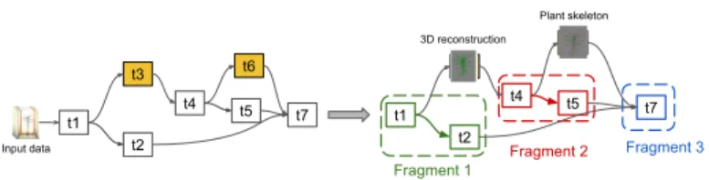
Figure 4 illustrates the preprocessing step on the Phenomenal SWf. The yellow tasks have their output data stored in the cache. They are replaced by the corresponding data as input for the subgraphs of tasks that need to be executed.
Fig. 4: DAG of tasks before pre-processing (left) and the selected fragments that need to be executed (right).
The second step, cache provisioning, is performed during workflow execution. Traditional (in memory) caching involves deciding, as data is read from disk into memory, which data to replace to make room, using a cache replacement algorithm, e.g. LRU. In our context, using a disk-based cache, the question is different, i.e. to decide which task output data to place in the cache using a cache provisioning algorithm. This algorithm is implemented by the cache manager and used by the task manager when executing a task.
A simple cache provisioning algorithm, which we will use as baseline, is to use a greedy method that simply stores all tasks’ output data in the cache. However, since SWf executions produce huge quantities of output data, this approach would incur high storage costs. Worse, for some short duration tasks, accessing cache data from disk may take much more time than re-executing the corresponding task subgraph from the input data in memory.
Thus, we propose a cache provisioning algorithm with an adaptive method that deals with the variations in task execution times and output data. The principle is to compute, for each task t, a score based on the sizes of the input and output data it consumes and produces, and the execution time of t. During workflow execution, the execution time of each task t, denoted by ExT ime(t), is stored in the provenance database. If t has already been executed, ExT ime(t) already exists in the provenance database. When t is re-executed, its execution time is recomputed and ExT ime(t) is updated as the average between the new and old execution times.
The adaptive aspect of our solution is to take into account task compression behavior. With a high compression ratio, it may be efficient to store the output data rather than the input data and recomputing it. In contrary, with a high expansion ratio, storing the input data rather than the output may save disk space.
Let size(Input(t)) and size(Output(t)) denote the input and output data size of a task t, respectively. The data compression ratio of a task quantifies the reduction of the input data processed by the task, i.e.,
CompressRatio(t) = size(Input(t))
size(Output(t)) (1)
Based on this data compression ratio, a cache provisioning score, denoted by CacheScore, is defined. For a task t, let F be a constant to normalize the time
factor, ωs and ωt represent the weight for the storage cost and execution time,
they are determined by the user and ωs+ ωt= 1, the cache provisioning score
is obtained by:
CacheScore(t) = ωs∗ CompressRatio(t) + ωt∗
Texec(t)
F (2)
The cache score reveals the relevancy of caching the output data of t and takes into account the compression metric and execution time. According to the weights provided by the user, she may prefer to give more importance to the compression ratio or executions time, depending on the storage capacity and available computational resources.
Then, during each task t execution, the task manager calls the cache manager to compute CacheScore(t). If the computed value is bigger than the threshold provided by the user, then t’s output data will be cached. This threshold is chosen based on the overhead of cache provisioning (i.e., the time spent to store t’s output data) and the cache size.
5
Experimental Evaluation
In this section, we first present our experimental setup. Then, we present our ex-periments and comparisons of different caching methods in terms of speedup and monetary cost in single user and multiuser modes. Finally, we give concluding remarks.
5.1 Experimental Setup
Our experimental setup includes the cloud infrastructure, SWf implementation and experimental dataset.
The cloud infrastructure is composed of one site with one data node (N1) and two identical compute nodes (N2, N3). The raw data is originally stored in an external server. During computation, raw data is transferred to N1, which contains Terabytes of persistent storage capacities. Each compute node has much computing power, with 80 vCPUs (virtual CPUs, equivalent to one core each of a 2.2GHz Intel Xeon E7-8860v3) and 3 Terabytes of RAM, but less persistent storage (20 Gigabytes).
We implemented the Phenomenal workflow (see Section 2) using OpenAlea and deployed it on the different nodes using the Conda multi-OS package man-ager. The master node is hosted on one of the compute node (N2). The metadata repositories are stored on the same node (N2) using the Cassandra key-value store. Files for raw and cached data are shared between the different nodes us-ing the Lustre file system. File transfer between nodes is implemented with ssh. The Phenoarch platform has a capacity of 1,680 plants with 13 images per plant per day. The size of an image is 10 Megabytes and the duration of an experiment is around 50 days. The total size of the raw image dataset represents 11 Terabytes for one experiment. The dataset is structured as 1,680 time series, composed of 50 time points (one per plant and per day).
We use a version of the Phenomenal workflow composed of 9 main activities.
We execute it on a subset of the use case dataset, that is 251 of the size of the
full datatset, or 440 Gigabytes of raw data, which represents the execution of 30,240 tasks.
5.2 Experiments
We execute the workflow on the subset dataset with different number of vCPUs and different caching methods. We consider workflow executions from a single user or multiple users to test the re-execution of the same workflow several times.
We compare three different caching methods: 1) no cache, 2) greedy, and 3) adaptive. Greedy and adaptive are described in Section 4.
In the single user scenario, the execution time corresponds to the transfer time of the raw data from the remote servers, the time to run the workflow and the time for cache provisioning, if any. In the multiuser scenario, the same workflow is executed on the same data several times (up to 6 times).
The raw data is fetched on the data node as follows: a first chunk is fetched from the remote data servers, then the remaining chunks are fetched while the execution starts on the first chunk. As the execution takes longer than transfer-ring the raw data, we only count the time of transfertransfer-ring the first chunk in the execution time.
For the adaptive method, the coefficients ωd and ωtdefined by the user are
set to 0.5 each. The threshold is set to 0.4.
20 40 60 80 100 120 140 160 # vCPUs 2 4 6 8 speedup No cache Greedy Adaptive
(a) Speedup for one execution
20 40 60 80 100 120 140 160 # vCPUs 0 5 10 15 20 25 speedup No cache Greedy Adaptive
(b) Speedup for three executions
Fig. 5: Speedup versus number of vCPUs: without cache (red), greedy caching (blue), and adaptive caching (green).
In the rest of this section, we compare the three methods in terms of speedup and monetary cost.
Speedup. We compare the speedup of the three caching methods. We define
speedup as speedup(n) = Tn
T10 where Tn is the execution time on n vCPUs and
T10 is the execution time of the no cache method on 10 vCPUs.
The workflow execution is distributed on nodes N2 and N3, for different numbers of vCPUs. For one execution, Figure 5.a shows that the fastest method is no cache (red curve). This is normal because there is no additional time to make data persistent and provision the cache. However, the overhead of cache provisioning with the adaptive method is very small (green curve in Figure 5.a) compared with the greedy method (blue curve in Figure 5.a) where all the output data are saved in the cache.
The speedup with adaptive goes up to 94.4% of that with no cache, while the speedup with greedy goes up to 59.9%. For instance, with 80 vCPUs, the
execu-tion time of the adaptive method (i.e., 3,714 seconds) is only 5.8% higher than that of the no cache method (i.e. 3,510 seconds). This is much faster than the greedy method, which adds 68.2% of computation time in comparison with the no cache method. Re-execution with the greedy and adaptive methods have much smaller execution time than the first execution. The greedy method re-execution time is the fastest, with only 2.3% (i.e., 129 seconds) of the no cache method ex-ecution time, because all the output data is already cached. Furthermore, as only the master node is working although no computation is done, the re-execution time is independent of the number of vCPUs and can be computed from a per-sonal computer with limited vCPUs. The adaptive method re-execution time is a bit higher as 16.3% (i.e., 572 seconds) of the no cache method execution time for a gain of 513%. With the adaptive method, some computation still needs to be done when the workflow is re-executed, but such re-execution on the whole dataset can be done in less than a day (i.e., 19.4 hours) on a 10 vCPUs machine, compared with 6.9 days with the no cache method. For three executions, starting without cache, Figure 5.b shows that the adaptive method is much faster than the other methods. The greedy method is faster than the no cache method in this case, because the additional time for the cache provisioning is compensated by the very short re-execution times of the greedy method. With 80 vCPUs, the speedup of the adaptive method (i.e., 18.1) is 54.70% better than that of the greedy method (i.e., 11.7) and 162.31% better than that of the no cache method (i.e., 6.9). The adaptive method is faster on three executions than the other methods, despite having re-execution time higher than the greedy method, because the overhead of the cache provisioning is 57% smaller.
Monetary Cost. To compare the monetary of the three caching methods, we first define execution cost in US$ as follows:
Cost = Costcpu∗ ExT ime + Costdisk∗ T otalCache
where ExT ime is the total time of one or multiple executions in seconds,
T otalCache represents the size of the data in the cache in Gigabytes. Costcpu
and Costdisk are the pricing coefficients determined in $ per cpu per hour and
$ per Gigabyte per month, respectively.
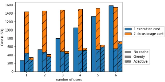
To set the price parameters, we use Amazon’s cost model, i.e., Costdisk is
$0.1 per Gigabyte per month for storage and two instances at $5.424 per hour for
computation, i.e., Costcpuis $10.848 per hour. As we can see from Figure 6, the
monetary cost of the adaptive method is much smaller than the greedy method due to the amount of cached data produced by the adaptive method (i.e., 390 Gigabytes for the whole experimentation), which is much smaller than for the greedy method (i.e., 3.9 % of the total output data). In terms of monetary cost, the greedy method becomes more efficient than the no cache method at the sixth user in the month. The adaptive method is 28.40% less costly than the no cache method and 254.44% less costly than the greedy method for two executions. For six executions, the adaptive method is still 120.16% less costly than no cache method and 114.38% less costly than the greedy method.
5.3 Discussion
The adaptive method has better speedup compared to the no cache and greedy methods, with performance gains up to 162.31% and 54.70% respectively for three executions. The direct execution time gain for each re-execution is 344.9% for the adaptive method in comparison with the no cache method (i.e., 3.9 hours instead of 17.7). One requirement from the use case was to make workflow execution time shorter than half a day (12 hours). The adaptive method allows for the user to re-execute the workflow on the total dataset (i.e., 11 Terabytes) in less than 4 hours. In terms of monetary costs, the adaptive method yields very good gains, up to 120.16% with 6 workflow re-executions in comparison to the no cache method and up to 254.44% for two workflow re-executions in comparison to the greedy method.
We also conducted other experiments based on the Phenomenal use case, typical of practical situations. However, because of space limitations, we can only summarize the results for two experiments: 1) execute a SWf that has al-ready been executed with different parameters, and 2) extend an existing SWf by adding new activities. The first experiment corresponds to the situation where the user tests other possibilities with different parameters. When some param-eters are changed, all the tasks depending on them and the one below need to be re-executed. For the greedy method, the overhead in cache provisioning and the storage cost increase rapidly as the number of parameters changes goes up. But the adaptive method has small overhead due to less data storage, and thus the increase of the storage cost is an order of magnitude smaller than that with greedy.
In the second experiment, the structure of the workflow is modified by adding new activities as discussed in Section 2. Similar to what happens with re-execution of a single SWf, the monetary cost of the greedy method is higher than the no cache method for up to 6 executions with different fragments or different parameters. And the execution time of greedy is always better than no cache. The adaptive method is both faster and cheaper than both no cache and greedy.
6
Conclusion
In this paper, we proposed an adaptive caching solution for efficient execution of data-intensive workflows in the cloud. Our solution automatically manages the storage and reuse of intermediate data and adapts to the variations in task execution times and output data size. The adaptive aspect our solution is to take into account task compression behavior.
We implemented our solution in the OpenAlea system and performed exten-sive experiments on real data with the Phenomenal workflow, with 11 Terabytes of raw data. We compared three methods : no cache, greedy, and adaptive. Our experimental validation shows that the adaptive method allows caching only the relevant output data for subsequent re-executions by other users, without incur-ring a high storage cost for the cache. The results show that adaptive caching can yield major performance gains, e.g., up to 120.16% with 6 workflow re-executions.
This work solves an important issue in experimental science like biology, where scientists extend existing workflows with new methods or new parameters to test their hypotheses on datasets that have been previously analyzed.
7
Acknowledgments
This work was supported by the #DigitAg French Convergence Lab. on Dig-ital Agriculture (http://www.hdigitag.fr/com), the SciDISC Inria associated team with Brazil, the Phenome-Emphasis project (ANR-11-INBS-0012) and IFB (ANR-11-INBS-0013) from the Agence Nationale de la Recherche and the France Grille Scientific Interest Group.
References
1. Adams, I.F., Long, D.D., Miller, E.L., Pasupathy, S., Storer, M.W.: Maximizing efficiency by trading storage for computation. In: HotCloud (2009)
2. Altintas, I., Barney, O., Jaeger-Frank, E.: Provenance collection support in the kepler scientific workflow system. In: International Provenance and Annotation Workshop. pp. 118–132 (2006)
3. Artzet, S., Brichet, N., Chopard, J., Mielewczik, M., Fournier, C., Pradal, C.: Openalea.phenomenal: A workflow for plant phenotyping (Sep 2018). https://doi.org/10.5281/zenodo.1436634
4. Callahan, S.P., Freire, J., Santos, E., Scheidegger, C.E., Silva, C.T., Vo, H.T.: Vistrails: visualization meets data management. In: ACM SIGMOD Int. Conf. on Management of Data (SIGMOD). pp. 745–747 (2006)
5. Cohen-Boulakia, S., Belhajjame, K., Collin, O., Chopard, J., Froidevaux, C., Gaig-nard, A., Hinsen, K., Larmande, P., Le Bras, Y., Lemoine, F., et al.: Scientific work-flows for computational reproducibility in the life sciences: Status, challenges and opportunities. Future Generation Computer Systems (FGCS) 75, 284–298 (2017) 6. Deelman, E., Singh, G., Livny, M., Berriman, B., Good, J.: The cost of doing science on the cloud: the montage example. In: International Conference forHigh Performance Computing, Networking, Storage and Analysis. pp. 1–12 (2008) 7. Garijo, D., Alper, P., Belhajjame, K., Corcho, O., Gil, Y., Goble, C.: Common
motifs in scientific workflows: An empirical analysis. Future Generation Computer Systems (FGCS) 36, 338–351 (2014)
8. Kelling, S., Hochachka, W.M., Fink, D., Riedewald, M., Caruana, R., Ballard, G., Hooker, G.: Data-intensive science: a new paradigm for biodiversity studies. BioScience 59(7), 613–620 (2009)
9. Liu, J., Morales, L.P., Pacitti, E., Costan, A., Valduriez, P., Antoniu, G., Mattoso, M.: Efficient scheduling of scientific workflows using hot metadata in a multisite cloud. IEEE Trans. on Knowledge and Data Engineering pp. 1–20 (2018)
10. Liu, J., Pacitti, E., Valduriez, P., Mattoso, M.: A survey of data-intensive scientific workflow management. Journal of Grid Computing 13(4), 457–493 (2015) 11. Ogasawara, E., Dias, J., Oliveira, D., Porto, F., Valduriez, P., Mattoso, M.: An
algebraic approach for data-centric scientific workflows. Proc. of the VLDB En-dowment (PVLDB) 4(12), 1328–1339 (2011)
12. de Oliveira, D., Bai˜ao, F.A., Mattoso, M.: Towards a taxonomy for cloud computing from an e-science perspective. In: Cloud Computing. Computer Communications and Networks., pp. 47–62. Springer (2010)
13. ¨Ozsu, M.T., Valduriez, P.: Principles of Distributed Database Systems, Third Edi-tion. Springer (2011)
14. Pradal, C., Artzet, S., Chopard, J., Dupuis, D., Fournier, C., Mielewczik, M., Ne-gre, V., Neveu, P., Parigot, D., Valduriez, P., et al.: Infraphenogrid: a scientific workflow infrastructure for plant phenomics on the grid. Future Generation Com-puter Systems (FGCS) 67, 341–353 (2017)
15. Pradal, C., Cohen-Boulakia, S., Heidsieck, G., Pacitti, E., Tardieu, F., Valduriez, P.: Distributed management of scientific workflows for high-throughput plant phe-notyping. ERCIM News 113, 36–37 (2018)
16. Roitsch, T., Cabrera-Bosquet, L., Fournier, A., Ghamkhar, K., Jim´enez-Berni, J., Pinto, F., Ober, E.S.: Review: New sensors and data-driven approaches—a path to next generation phenomics. Plant Science (2019)
17. Tardieu, F., Cabrera-Bosquet, L., Pridmore, T., Bennett, M.: Plant phenomics, from sensors to knowledge. Current Biology 27(15), R770–R783 (2017)
18. Yuan, D., Yang, Y., Liu, X., Chen, J.: A cost-effective strategy for intermediate data storage in scientific cloud workflow systems. In: IEEE Int. Symp. on Parallel & Distributed Processing (IPDPS). pp. 1–12 (2010)
19. Yuan, D., Yang, Y., Liu, X., Li, W., Cui, L., Xu, M., Chen, J.: A highly practical approach toward achieving minimum data sets storage cost in the cloud. IEEE Trans. on Parallel and Distributed Systems 24(6), 1234–1244 (2013)
20. Zhang, J., Votava, P., Lee, T.J., Chu, O., Li, C., Liu, D., Liu, K., Xin, N., Nemani, R.: Bridging vistrails scientific workflow management system to high performance computing. In: 2013 IEEE Ninth World Congress on Services. pp. 29–36. IEEE (2013)