EUROPEAN ORGANISATION FOR NUCLEAR RESEARCH (CERN)
JHEP 03 (2020) 145
DOI:10.1007/JHEP03(2020)145
CERN-EP-2019-162 3rd July 2020
Search for new resonances in mass distributions of
jet pairs using 139 fb
√
−1
of
p p collisions at
s
= 13 TeV with the ATLAS detector
The ATLAS Collaboration
A search for new resonances decaying into a pair of jets is reported using the dataset of proton–proton collisions recorded at
√
s = 13 TeV with the ATLAS detector at the Large Hadron Collider between 2015 and 2018, corresponding to an integrated luminosity of 139 fb−1. The distribution of the invariant mass of the two leading jets is examined for local excesses above a data-derived estimate of the Standard Model background. In addition to an inclusive dijet search, events with jets identified as containing b-hadrons are examined specifically. No significant excess of events above the smoothly falling background spectra is observed. The results are used to set cross-section upper limits at 95% confidence level on a range of new physics scenarios. Model-independent limits on Gaussian-shaped signals are also reported. The analysis looking at jets containing b-hadrons benefits from improvements in the jet flavour identification at high transverse momentum, which increases its sensitivity relative to the previous analysis beyond that expected from the higher integrated luminosity.
© 2020 CERN for the benefit of the ATLAS Collaboration.
Reproduction of this article or parts of it is allowed as specified in the CC-BY-4.0 license.
1 Introduction
Many models of physics beyond the Standard Model (SM) predict the existence of new heavy particles which couple to quarks and/or gluons. Such heavy particles could be produced in proton–proton collisions at the Large Hadron Collider (LHC) and then decay into quarks and gluons, creating two energetic jets in the detector. In the SM, dijet events are produced mainly by quantum chromodynamics (QCD) processes. QCD predicts dijet events with a smoothly decreasing invariant mass distribution, mjj. A new particle
decaying into quarks or gluons would emerge instead as a resonance in the mjjspectrum.
If the new particle has a sizeable coupling to b-quarks and decays into b ¯b, bq or bg pairs, the identification of jets containing b-hadrons (b-tagging) in the decay final state could significantly enhance the sensitivity to such a new particle. This analysis searches for resonant excesses in the mjjdistribution of the two most
energetic jets with an inclusive jet selection and with separate selections where at least one or exactly two jets are identified as containing a b-hadron.
Dijet resonance searches have been performed at previous hadron colliders covering the dijet invariant mass range from 110 GeV to 1.4 TeV [1–4]. At the LHC, the most recent searches probe masses up to 7.5 TeV [5, 6]. The lowest inspected mjjvalue in the recent LHC searches is above 1 TeV and is dictated by the trigger
and data-acquisition systems of the experiments. Searching for resonances below the TeV mass range is well motivated and alternative approaches employing more sophisticated trigger or analysis strategies have resulted in novel searches [7–12]. For new resonances decaying into jets containing b-hadrons, dedicated searches have been performed [13,14].
In this analysis, the dataset recorded at √
s = 13 TeV with the ATLAS detector is used, corresponding to an integrated luminosity of 139 fb−1. The mjjspectrum ranging from 1.1 TeV to 8 TeV is probed, and the
results are interpreted in the context of several new physics scenarios, which include excited quarks q∗ (q = (u, d, c, s, b)) from compositeness models [15,16]; heavy Z0and W0gauge bosons [17–19]; a chiral excitation of the W boson, denoted W∗[20,21]; a leptophobic Z0dark-matter mediator model [22–24]; quantum black holes [25, 26]; and Kaluza–Klein gravitons [27, 28]. In addition, limits on generic Gaussian-shaped narrow-resonance signals [29] are derived.
2 ATLAS detector
The ATLAS detector [30] at the LHC covers nearly the entire solid angle around the collision point.1 It consists of an inner tracking detector surrounded by a thin superconducting solenoid, electromagnetic and hadronic calorimeters, and a muon spectrometer incorporating three large superconducting toroidal magnets. The inner-detector system is immersed in a 2 T axial magnetic field and provides charged-particle tracking in the range |η| < 2.5.
The high-granularity silicon pixel detector covers the vertex region and typically provides four measurements per track, the first hit normally being in the insertable B-layer installed before Run 2 [31,32]. It is followed by the silicon microstrip tracker which usually provides eight measurements per track. These silicon
1 ATLAS uses a right-handed coordinate system with its origin at the nominal interaction point (IP) in the centre of the detector and the z-axis along the beam pipe. The x-axis points from the IP to the centre of the LHC ring, and the y-axis points upwards. Cylindrical coordinates (r, φ) are used in the transverse plane, φ being the azimuthal angle around the z-axis. The pseudorapidity
detectors are complemented by the transition radiation tracker, which enables radially extended track reconstruction up to |η| = 2.0 and contributes to electron identification.
The calorimeter system covers the pseudorapidity range |η| < 4.9. Within the region |η| < 3.2, electromagnetic calorimetry is provided by barrel and endcap high-granularity lead/liquid-argon (LAr) calorimeters, with an additional thin LAr presampler covering |η| < 1.8, to correct for energy loss in material upstream of the calorimeters. Hadronic calorimetry is provided by the steel/scintillator-tile calorimeter, segmented into three barrel structures within |η| < 1.7, and two copper/LAr hadronic endcap calorimeters. The solid angle coverage is completed with forward copper/LAr and tungsten/LAr calorimeter modules optimised for electromagnetic and hadronic measurements, respectively.
The outermost layers of ATLAS consist of an external muon spectrometer within |η| < 2.7, incorporating three large toroidal magnet assemblies with eight coils each.
Interesting events were selected to be recorded by the first-level trigger system implemented in custom hardware, followed by selections made by algorithms implemented in software in the high-level trigger computer farm [33]. The first-level trigger reduces the selection rate from the 40 MHz bunch crossing rate to below 100 kHz, which the high-level trigger further reduces in order to record events to disk at a rate of about 1 kHz.
3 Simulated event samples
Monte Carlo (MC) simulations are used to model the expected benchmark signals and to validate the SM background estimation.
In most of the sample generation, the leading-order (LO) NNPDF2.3 parton distribution functions (PDF) [34] and the A14 Pythia tuned parameter set for the modelling of parton showers, hadronisation and the underlying event [35] were adopted, unless otherwise described below.
MC events from QCD multijet processes were generated with Pythia v8.186 [36]. The renormalisation and factorisation scales were set to the average transverse momentum pTof the two leading (highest pT)
jets. Generated events were reweighted to next-to-leading-order (NLO) predictions using mjj-dependent
correction factors [37–39]. To validate the modelling of the background, the MC simulation is normalized to the data and the shapes of various kinematic variables in simulation are compared with the data. The MC simulation is found to agree with the data, with a difference of up to approximately 20% in the tail regions.
Due to the limited size of the simulated samples and the large theoretical uncertainties of QCD processes, the background is estimated by fitting each of the data mjjspectra as described in Section5.
Several models of new physics were simulated, including heavy gauge bosons, a chiral excitation of the W boson, excited quarks, quantum black holes and Kaluza–Klein gravitons. The sequential standard model (SSM) Z0boson [17] has the same couplings to the SM fermions as the SM Z boson, so the bottom-quark decay branching fraction B(Z0→ b ¯b) is 13.8%. The intrinsic width of the SSM Z0boson is approximately 3% of the resonance mass. Events from the SSM Z0model were generated in the b ¯b decay channel with Pythia v8.186 at LO, and the cross-sections were then corrected to the NLO predictions [40].
A leptophobic Z0model with axial-vector couplings to SM quarks and containing a Dirac fermion dark matter (DM) candidate is considered [24]. The events from Z0decaying into q ¯q where q = (u, d, s, c, b)
were generated with MadGraph5_aMC@NLO 2.4.3 [40] with the DM mass fixed to 10 TeV and the coupling to dark matter (gχ) set to 1.5. The mediator Z0mass ranges from 1 TeV to 7 TeV, and the coupling to SM quarks (gq) varies from 0.1 to 0.5. In this scenario, the Z
0
does not decay into the DM candidate and so the dijet signal depends only upon the coupling to quarks and the mass of the Z0resonance. The chosen gq= 0.5 coupling corresponds to a width of 12% of the resonance mass, nearly the maximum width to which this search is sensitive. For the resonance searches with b-tagging, dedicated samples of Z0signals decaying into b ¯b final states were simulated using the same generator set-up as for the inclusive samples. In this leptophobic case, the bottom-quark decay branching fraction B(Z0→ b ¯b) is 18.9%.
A heavy charged W0gauge boson model [19] with V − A couplings was simulated similarly to the SSM Z0 scenario, using Pythia v8.186 at LO. The mass of the W0ranges from 1 TeV to 6.5 TeV and only hadronic decays of the W0were simulated, with all six quark flavours included.
Events with a chiral excitation of the W boson, W∗, arising from a W compositeness model [20, 21], were generated with CalcHep v3.6 [41], and then processed with Pythia v8.210 for the simulation of non-perturbative effects. The angular distribution of the decay products differs strongly from those of all other models considered in this analysis and has an excess more towards the forward region, which motivates using a different kinematic selection for this signal. The decays of the W∗ were set to be leptophobic and include all SM quarks. Event samples of W∗bosons were generated with masses ranging from 1.8 TeV to 6.0 TeV.
Excited quark (q∗) signal samples [15,16] were generated with Pythia v8.186, assuming spin-½ excited quarks with the same coupling constants as SM quarks. Both light flavour (u, d, s) and heavy flavour (c, b) quarks were taken into account in the event generation. The generated q∗masses range from 2 TeV to 8 TeV. The compositeness scale was set to the excited-quark mass. Only the decay into a gluon and an up-or down-type quark was simulated; this is the dominant process in the dijet final state, with a branching ratio of 85%. Excited b-quark (b∗) signal samples were produced specifically for searches in the b-tagged dijet categories. The same mass range as for the q∗signal samples was simulated with analogous generator settings. All decay modes were simulated with the dominant mode being the bg channel, with a branching fraction of 85%, and the remaining decay modes being bγ, bZ and tW .
In models with large extra dimensions [42], the fundamental scale of gravity MDis lowered to a few TeV.
Quantum black holes (QBH) [25,26], the quantum analogues of ordinary black holes, can be produced at or above this scale at the LHC. Once produced, QBH would decay into two-body final states, mainly jets. Events from a QBH model were generated with BlackMax [43] for six extra dimensions, using the CTEQ6L1 PDF set [44] and with MDranging from 4 TeV to 10 TeV.
In the Randall–Sundrum extra dimension model [27,28], the Kaluza–Klein (KK) spin-2 graviton decays preferentially into gluons and quarks. Graviton signal samples were generated with Pythia v8.212 assuming the curvature parameter k/MPL = 0.2, where MPLis the four-dimensional reduced Planck scale.
The KK graviton samples were simulated in the G → b ¯b decay mode, with masses ranging from 1.25 TeV to 7 TeV.
The generated background samples from QCD processes were passed through a full ATLAS detector simulation [45] using Geant 4 [46]. The signal MC samples were passed through a fast simulation which relies on a parameterisation of the calorimeter response [47]. The decay of b- and c-hadrons was performed consistently using the EvtGen v1.2.0 decay package [48]. To account for additional proton–proton interactions (pile-up) from the same and neighbouring bunch crossings, a number of inelastic pp interactions were generated with Pythia v8.186 using the NNPDF23LO PDF set [49] and the ATLAS
simulated events were weighted so that the distributions of the average number of collisions per bunch crossing in simulation and in data match.
4 Data and event selection
The data for this analysis were collected by the ATLAS detector from pp collisions at the LHC with a centre-of-mass energy of
√
s = 13 TeV in the years from 2015 to 2018. With requirements that all detector systems were functional and recording high-quality data, the dataset corresponds to an integrated luminosity of 139 fb−1. The uncertainty in the combined 2015–2018 integrated luminosity is 1.7% [51], obtained using the LUCID-2 detector [52] for the primary luminosity measurements. Events are selected using a trigger that requires at least one jet with pTgreater than 420 GeV, the lowest-pT non-prescaled
single-jet trigger.
Collision vertices are reconstructed from at least two tracks with pT > 0.5 GeV. The primary vertex is
selected as the one with the highestÍ p2Tof the associated tracks.
In event reconstruction, calorimeter cells with an energy deposit significantly above the calorimeter noise are grouped together according to their contiguity to form topological clusters [53]. These are then grouped into jets using the anti-ktalgorithm [54,55] with a radius parameter of R = 0.4. Jet energies and directions are corrected by jet calibrations as described in Ref. [56]. Events are rejected if any jet with pT > 150 GeV
is compatible with noise bursts, beam-induced background or cosmic rays using the ‘loose’ criteria defined in Ref. [57].
Jets containing a b-hadron are identified using a deep-learning neural network, DL1r, for the first time at ATLAS. The DL1r b-tagging is based on distinctive features of b-hadrons in terms of the impact parameters of tracks and the displaced vertices reconstructed in the inner detector. The inputs of the DL1r network also include discriminating variables constructed by a recurrent neural network (RNNIP) [58], which exploits the spatial and kinematic correlations between tracks originating from the same b-hadron. This approach is found chiefly to improve the performance for jets with high pT [59]. Operating points are
defined by a single cut-value on the discriminant output distribution and are chosen to provide a specific b-jet efficiency for an inclusive t ¯t MC sample. A 77% efficiency b-tagging operating point is adopted, which gives maximal overall signal sensitivity across the various signal models and masses considered in the b-tagged categories. The b-tagging performance has a strong dependence on the jet pT: the efficiency
drops from 65% for a b-jet pTof around 500 GeV to 10% for a pTof around 2 TeV. Estimated from MC
simulation, the corresponding mis-tag rate of charm jets drops from 15% to 2% over the same pTinterval,
and that of light-flavour jets remains at the level of 1%. Simulation-to-data scale factors are applied to the simulated event samples to compensate for differences in the b-tagging efficiency between data and simulation. These scale factors are measured as a function of jet pTusing a likelihood-based method in
a sample highly enriched in t ¯t events [60]. Given that the number of b-jets in data is limited for jet pT
> 400 GeV, additional uncertainties are assessed by varying in the simulation the underlying quantities that are known to affect the b-tagging performance. The differences between the b-tagging efficiency after each variation and the nominal b-tagging efficiency are then used to construct an extrapolation uncertainty to extend the validity of the correction factors into the higher jet-pT range used in this analysis. The
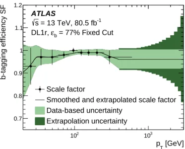
simulation-to-data scale factor as a function of jet pTfor the 77% operating point of the DL1r b-tagging
algorithm adopted in this search is shown in Figure1. More details about the procedure for the extraction and extrapolation of the b-tagging scale factors can be found in Ref. [60].
[GeV] T p 2 10 103 b-tagging efficiency SF 0.7 0.8 0.9 1 1.1 1.2 Scale factor
Smoothed and extrapolated scale factor Data-based uncertainty Extrapolation uncertainty ATLAS -1 = 13 TeV, 80.5 fb s = 77% Fixed Cut b ε DL1r,
Figure 1: Simulation-to-data scale factor as a function of jet pTfor the 77% operating point of the DL1r b-tagging algorithm. The scale factors are measured with a likelihood-based method in a sample highly enriched in t ¯t events using 2015–2017 data, as described in Ref. [60], with uncertainties due to the limited size of data sample, detector calibration and physics modelling. An additional uncertainty is included to extrapolate the measured uncertainties to the high-pTregion of interest (pT> 400 GeV), and has contributions related to the reconstruction of tracks and jets, the modelling of the b-hadrons and the interaction of long-lived b-hadrons with the detector material.
The analysis selections and the corresponding signal models investigated are summarised in Table1. Events must contain at least two jets with pT greater than 150 GeV and the azimuthal angle between the two
leading jets must be greater than 1.0. To maximise the sensitivities to various signal models, the events are classified into an inclusive category with no b-jet tagging requirement, a one-b-tagged category (1b), requiring at least one of the two leading jets to be b-tagged, and a two-b-tagged category (2b), with both of the two leading jets being b-tagged. For categories selecting b-jets, the two leading jets must be within |η| < 2.0.
To reduce the dominant background contribution from QCD processes, a selection based on half of the rapidity separation between the two leading jets, y∗= (y1− y2)/2, is implemented, where y1and y2are the
rapidities of the leading jet and subleading jet respectively. The signal dijet events are produced through s-channel processes, which favour small |y∗|, while a large fraction of the background events are from QCD t-channel processes and have large | y∗|. The |y∗| cut values are optimised for various categories and signals. In the inclusive selection, | y∗|< 0.6 is required for the considered signals, except W∗. Due to the fact that a larger | y∗| is favoured in the W∗decays, a looser requirement | y∗| < 1.2 is adopted in the search for W∗signals. In the b-tagged categories, where the two leading jets have |η| < 2.0, a selection | y∗| < 0.8 is made.
A lower bound on the dijet invariant mass mjjis required to ensure a fully efficient selection without any
kinematic bias; it is determined by the single-jet trigger’s efficiency turn-on and also depends on the | y∗| requirement, as shown in Table1. Within the acceptance of the mjjand | y
∗| selections, the leading jet’s
pTis above the single-jet trigger’s threshold. For the inclusive selection, the acceptance of QBH and q∗ signals is around 55% for all the masses considered, while that of W0and Z0ranges from approximately 20% to 45%, depending on the resonance mass. For the W∗selection, the acceptance increases from 30%
to 70% for W∗mass values from 2 TeV to 6 TeV. For the b-tagged categories, the acceptance of b∗and Z0(b ¯b) increases from 20% and reaches a plateau of around 70% at a mass of 2.5 TeV.
The signal selection efficiencies from the b-tagging requirement (per-event b-tagging efficiencies) shown in Figure2are derived after applying the rest of the event selection. The efficiency decreases as mjjincreases,
since the b-tagging efficiency decreases when the jet pT increases. In the 1b category, the efficiency for
final states containing two b-quarks, such as a Z0signal, is higher than for the b∗signal. At high mass, because the gluon from the b∗decay is more likely to split into a b ¯b pair, the per-event b-tagging efficiency of the b∗signal is enhanced and closer to what is observed in simulated Z0events.
[TeV]
jj
m 1 1.5 2 2.5 3 3.5 4 4.5 5
Event Tagging Efficiency
0 0.2 0.4 0.6 0.8 1 1 b-tag ≥ ), b DM mediator Z'(b 1 b-tag ≥ b*, ), 2 b-tag b DM mediator Z'(b
ATLAS Simulation, s = 13 TeV
DL1r, Fixed cut 77% WP
Figure 2: The probability of an event to pass the b-tagging requirement after the rest of the event selection, shown as a function of the resonance mass mjjand for the 1b and 2b analysis categories.
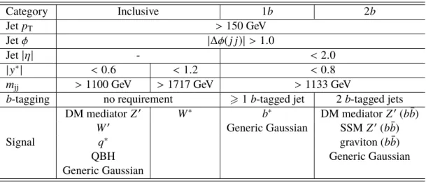
Table 1: Summary of the event selection requirements and benchmark signals being tested in each analysis category. Only the two jets with highest pTenter in the event selection. The exact values of the mjjlower bounds also depend on the jet energy resolution uncertainty.
Category Inclusive 1b 2b
Jet pT > 150 GeV
Jet φ |∆φ(j j)| > 1.0
Jet |η| - < 2.0
| y∗| < 0.6 < 1.2 < 0.8
mjj > 1100 GeV > 1717 GeV > 1133 GeV
b-tagging no requirement > 1 b-tagged jet 2 b-tagged jets
Signal DM mediator Z0 W∗ b∗ DM mediator Z0(b ¯b) W0 Generic Gaussian SSM Z0(b ¯b) q∗ graviton (b ¯b) QBH Generic Gaussian Generic Gaussian
5 Dijet mass spectrum
The SM production of dijet events is dominated by QCD multijet processes, which yield a smoothly falling mjjspectrum. To determine the SM contribution, the sliding-window fitting method [5] is applied to the data, with a nominal fit using a parametric function:
f (x)= p1(1 − x)p2xp3+p4ln x
where x = mjj/
√
s and p1,2,3,4are the four fitting parameters. The background in each mjjbin is extracted
from the data by fitting in a mass window centred around that bin. The window size is chosen to be the largest possible window that satisfies the fit requirements described later in this section.
Several data-driven background mjjspectra are used to validate the background fitting strategy. On these
spectra, ‘signal injection tests’ and ‘spurious signal tests’ are performed to validate the sliding-window fit. For the b-tagged categories, the background-only spectra are derived from control regions (CRs) which are constructed by reversing the requirement on | y∗| or removing the b-tagging requirement. In these CRs the signal leakage is expected to be small, and this is confirmed by the MC simulation. In the CRs with the | y∗| < 0.8 requirement reversed, per-event fractions passing b-tagging selections are derived as functions of pT and η of the two leading jets for both the 1b and 2b categories, which fully take into
account the correlations between the leading and subleading jets. The dijet spectra from QCD processes in the b-tagged signal regions are obtained from the CR with no b-tagging requirement (using the signal region | y∗| selection), multiplied by the appropriate b-tagging efficiencies. For the inclusive category, in the absence of a background-dominated control region, a test spectrum corresponding to an integrated luminosity of 139 fb−1is created to perform these tests by scaling up the background-only fit to the 37 fb−1 dataset, which is already published in Ref. [5] with no evidence of new physics, and then fluctuating the content of each bin around the fit value according to a Poisson distribution. No significant bias is observed in the tests, as described below.
In the signal injection tests, various signal models are added to the expected background distribution to assess whether or not the sliding-window procedure is able to fit the combined distribution and measure the correct signal yield. This test is designed to evaluate how sensitive the sliding-window fit is to all the tested signal types. For each of the benchmark and Gaussian-shaped signals, the extracted signal yield is consistent with that injected within the statistical uncertainty.
In the spurious signal tests, signal-plus-background fits are run on the background-only spectra for different signal masses and the extracted signal yield is taken as an estimate of the spurious signal. This test evaluates the robustness of the background fitting strategy and the capability of the fit function to model the background. All signals considered for the inclusive categories show no bias, with the exception of Gaussian-shaped resonances with relative widths of 15% where a spurious signal yield of up to 12% of the statistical uncertainty of the estimated background from the fit is observed at high mass, where data counts are limited. In the b-tagged categories, the spurious signal yield observed for all the signals considered is between 10% and 20% of the statistical uncertainty of the estimated background fit. A corresponding systematic uncertainty is assigned for affected signals as described in Section6.
The statistical significance of any localised excess in the mjjdistribution is quantified using the BumpHunter
test [61, 62]. The BumpHunter calculates the significance of any excess found in continuous mass intervals in all possible locations of the binned mjjdistribution. The search window’s width varies from a
the scan, BumpHunter computes the significance of the difference between the data and the background. The interval that deviates most significantly from the smooth spectrum is defined by the set of bins that have the smallest probability of arising from a Poisson background fluctuation. The probability of random fluctuations in the background-only hypothesis to create an excess at least as significant as the one observed anywhere in the spectrum, the BumpHunter p-value, is determined by performing a series of pseudo-experiments drawn from the background estimate, with the look-elsewhere effect [63] considered. The fitting quality is assessed via the BumpHunter p-value. In a good fit, any localised excess is expected to arise from fluctuations in the fitted background distribution. In determining the window size of the sliding-window fit, a fit is accepted if the corresponding BumpHunter p-value is greater than 0.01. Figure3shows the observed mjjdistributions for the various categories. The bin widths for each category
are chosen to approximate the mjjresolution, which broadens with increasing mjjmass. Predictions for
benchmark signals are scaled to larger cross-sections, from 10 to 1000 times their expected values, for display purposes. The vertical lines indicate the most discrepant interval identified by the BumpHunter test. No significant deviation from the background-only hypothesis is observed in the data spectra. In the inclusive category, the BumpHunter p-values of the most discrepant regions are 0.89 for dijet events with | y∗| < 0.6 and 0.88 for events with |y∗| < 1.2. In the b-tagged categories, the BumpHunter p-values of the most discrepant regions are 0.69 for 1b and 0.83 for 2b. The lower panel in each plot of Figure3 shows the significance of the bin-by-bin differences between the data and the fit, as calculated from Poisson probabilities, considering only statistical uncertainties.
6 Systematic uncertainties
The statistical uncertainty of the fit due to the limited size of the data sample and the uncertainty due to the choice of fit function are considered as systematic uncertainties affecting the data-driven background determination.
To estimate these uncertainties, a large number of pseudo-data sets (∼ 10 000) are generated as Poisson fluctuations from the nominal distribution. The statistical uncertainty in the values of the parameters in the fit function is derived by repeating the sliding-window fitting procedure on the pseudo-data. The uncertainty in each mjjbin is taken to be the root mean square of the fit results in that bin for all pseudo-experiments,
which increases from approximately 0.1% at mjj= 2 TeV to 30%–40% in the high mjjtail region. These
uncertainties, and the ones throughout this Section, are expressed as variations relative to the nominal values.
The uncertainty due to the choice of background parameterisation is estimated by fitting the pseudo-data with the nominal function and alternative parametric functions. To determine the alternative functional form, several fits are performed using variations of the nominal function with at most one additional free parameter. The functional form used to estimate the systematic uncertainty is taken as the function giving the largest difference from the nominal fit while still fulfilling the fit quality criteria. For the inclusive category, the alternative function has the form p1(1 − x)p2xp3+p4ln x+p5xwhile for the b-tagged categories,
where the b-tagging efficiency biases the mjjdistribution, the form p1(1 − x)p2+p3xxp4+p5ln xis adopted.
The difference between the alternative background prediction and the nominal one, averaged across the set of pseudo-data, is considered as a systematic uncertainty, which reaches 10% in the highest mass regions investigated in this analysis.
1 2 3 4 5 6 7 8 [TeV] jj Reconstructed m 1 − 10 1 10 2 10 3 10 4 10 5 10 6 10 7 10 8 10 9 10 Events 1 2 3 4 5 6 7 8 [TeV] jj m 2 − 0 2 Significance ATLAS -1 =13 TeV, 139 fb s Inclusive Data Background fit BumpHunter interval = 4 TeV * q *, m q = 6 TeV * q *, m q -value = 0.89 p 10 × σ *, q (a) 2 3 4 5 6 7 8 9 [TeV] jj Reconstructed m 1 − 10 1 10 2 10 3 10 4 10 5 10 6 10 7 10 8 10 9 10 Events 2 3 4 5 6 7 8 9 [TeV] jj m 2 − 0 2 Significance ATLAS -1 =13 TeV, 139 fb s W* Selection Data Background fit BumpHunter interval = 4 TeV W* W*, m = 5 TeV W* W*, m -value = 0.88 p 1000 × σ W*, (b) 2 3 4 5 6 [TeV] jj Reconstructed m 1 − 10 1 10 2 10 3 10 4 10 5 10 6 10 7 10 8 10 Events 2 3 4 5 6 [TeV] jj m 2 − 0 2 Significance ATLAS -1 =13 TeV, 139 fb s 1 b-tag ≥ Data Background fit BumpHunter interval = 2 TeV * b *, m b = 3 TeV * b *, m b -value = 0.69 p 100 × σ *, b (c) 1.5 2 2.5 3 3.5 4 4.5 [TeV] jj Reconstructed m 1 − 10 1 10 2 10 3 10 4 10 5 10 6 10 7 10 Events 1.5 2 2.5 3 3.5 4 4.5 [TeV] jj m 2 − 0 2 Significance ATLAS -1 =13 TeV, 139 fb s 2 b-tag Data Background fit BumpHunter interval = 2 TeV Z' DM Z', m = 3 TeV Z' DM Z', m -value = 0.83 p 10 × σ =0.25, q DM Z' g (d)
Figure 3: Dijet invariant mass distributions from multiple categories: (a) inclusive dijet with | y∗|< 0.6, (b) inclusive dijet with | y∗|< 1.2, (c) dijet with at least one b-tagged jet and (d) dijet with both jets b-tagged. The vertical lines indicate the most discrepant interval identified by the BumpHunter test, for which the p-value is stated in the figure.
An additional systematic uncertainty is considered, based on the spurious signal tests. In the inclusive category, this systematic uncertainty is required only for the Gaussian-shaped signal with a width of 15% of its mass, since for the other signal hypotheses no bias is seen. For the b-tagged categories, this uncertainty is considered for each signal according to the size of the observed effect. The effect of this uncertainty on the signal cross-sections is found to be less than 5% of the excluded values for all benchmark and Gaussian-shaped signals considered.
The main systematic uncertainties in the MC signal samples include those associated with the modelling of the jet energy scale (JES), the jet energy resolution (JER) and the b-tagging efficiency. JES and JER variations are applied to all the signals and affect the signal templates. They are estimated using jets in 13 TeV data and simulation in various methods as described in Ref. [56]. The JES uncertainty is less than 2% of the jet pTfor dijet invariant mass below 5 TeV and around 4% for higher mass. The JER uncertainty
ranges from 3% to 6% across the whole dijet invariant mass range investigated.
In the categories selecting one or two jets from b-hadrons, the systematic uncertainty of the b-tagging efficiency dominates. The uncertainty is measured using data enriched in t ¯t events for jet pT < 400 GeV
and extrapolated to higher-pTregions [60]. Dedicated simulations are used to extrapolate the measured
uncertainties to the high-pTregion of interest. Contributions related to the reconstruction of tracks and jets,
the modelling of the b-hadrons and the interaction of long-lived b-hadrons with the detector material are considered. Among the uncertainties associated with the reconstruction of tracks, those found to affect the b-tagging performance the most are the ones related to the track impact-parameter resolution, the fraction of fake tracks, the description of the detector material, and the track multiplicity per jet. The uncertainty increases from 2% for a jet pTof around 90 GeV to 20% for a jet pTof around 3 TeV. The overall b-tagging
uncertainty affecting the normalisation of the Gaussian-shaped signals is taken into account.
A luminosity uncertainty of 1.7% is applied to the normalisation of the signal samples. Uncertainties in the signal acceptance associated with the choice of PDF and the scale choices are found to be approximately 1% for most signals, reaching 4% for high mass values.
7 Signal interpretation
Since no significant deviation from the expected background is observed, constraints on various signal models that would produce a resonance in the dijet invariant mass distribution are derived using a frequentist framework [64]. Upper limits on the signal cross-section times acceptance times branching ratio are extracted at 95% confidence level (CL) using the CLsmethod [65] with a binned profile likelihood ratio as
the test statistic. For the 1b and 2b categories, the upper limits are set on the signal cross-section times acceptance times b-tagging selection efficiency times branching ratio. The expected limits are calculated with the asymptotic approximation to the test statistic’s distribution [66] and using pseudo-experiments generated according to the values of the background uncertainties from the maximum-likelihood fit. Pseudo-experiments are employed for the interpretation of the signals populating the high-mass part of the spectra where the relative deviation from the asymptotic approximation is found to be more than 1%. The calculated limits are logarithmically interpolated. No uncertainty is applied to the signal theoretical cross-sections. The systematic uncertainties of the background and signal samples are incorporated into the limits by varying all the uncertainty sources according to Gaussian probability distributions. For the signal models considered here, the new physics resonance’s couplings are strong compared with the scale of perturbative QCD at the signal mass, so that the interference with QCD terms can be neglected.
2 3 4 5 6 7 8 [TeV] q* m 5 − 10 4 − 10 3 − 10 2 − 10 1 − 10 1 BR [pb] × A × σ Theory Observed 95% CL Expected 95% CL σ 1 ± σ 2 ± ATLAS -1 = 13 TeV, 139 fb s q*, inclusive (a) 4 5 6 7 8 9 10 [TeV] QBH m 6 − 10 5 − 10 4 − 10 3 − 10 2 − 10 1 − 10 1 BR [pb] × A × σ Theory Observed 95% CL Expected 95% CL σ 1 ± σ 2 ± ATLAS -1 = 13 TeV, 139 fb s QBH, inclusive (b) 2 3 4 5 6 [TeV] W' m 4 − 10 3 − 10 2 − 10 1 − 10 1 BR [pb] × A × σ Theory Observed 95% CL Expected 95% CL σ 1 ± σ 2 ± ATLAS -1 = 13 TeV, 139 fb s W', inclusive (c) 2 2.5 3 3.5 4 4.5 5 5.5 6 [TeV] W* m 4 − 10 3 − 10 2 − 10 1 − 10 1 BR [pb] × A × σ Theory Observed 95% CL Expected 95% CL σ 1 ± σ 2 ± ATLAS -1 = 13 TeV, 139 fb s W*, inclusive (d)
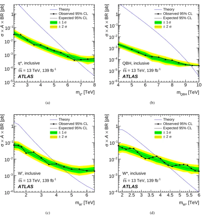
Figure 4: The 95% CL upper limits on the cross-section times acceptance times branching ratio into two jets as a function of the mass of (a) q∗, (b) QBH, (c) W0and (d) W∗signals. The expected upper limit and corresponding ±1σ and ±2σ uncertainty bands are also shown. These exclusion upper limits are obtained using the inclusive dijet selection, with the selection described in the text and summarised in Table1.
Table 2: The lower limits on the masses of benchmark signals at 95% CL.
Category Model Lower limit on signal mass at 95% CL
Observed Expected Inclusive q∗ 6.7 TeV 6.4 TeV QBH 9.4 TeV 9.4 TeV W0 4.0 TeV 4.2 TeV W∗ 3.9 TeV 4.1 TeV
DM mediator Z0, gq= 0.20 3.8 TeV 3.8 TeV
DM mediator Z0, gq= 0.50 4.6 TeV 4.9 TeV
1b b∗ 3.2 TeV 3.1 TeV
2b
DM mediator Z0gq= 0.20 2.8 TeV 2.8 TeV
DM mediator Z0, gq= 0.25 2.9 TeV 3.0 TeV
SSM Z0, 2.7 TeV 2.7 TeV
graviton, k/MPL= 0.2 2.8 TeV 2.9 TeV
The upper limits obtained from the inclusive category for the signal cross-sections of q∗, QBH, W0and W∗ are shown in Figure4. The constraints on the leptophobic DM mediator Z0model are shown in Figure5. For the upper limits on the universal coupling gqof the Z
0
model, signal points are simulated with 0.5 TeV spacing in mass and spacing as fine as 0.05 in gq. A smooth curve is drawn between points by interpolating
in gqfollowed by an interpolation in Z 0
mass. For a given mass, the cross-sections rise with gq, and thus
the upper-left unfilled area is excluded. The upper limits on the signal yields from the 1b category for the b∗signal are shown in Figure6and those from the 2b category for the Z0and graviton signals are shown in Figure7. The lower limits on the signal masses for each of the benchmark models are summarised in Table2. For the leptophobic DM mediator Z0 model the signal constraint from the 2b category is comparable to that from the inclusive category at a signal mass of around 1.5 TeV, and weaker at higher masses mainly due to the loss of b-tagging efficiency. For new states with a larger branching ratio into b-quark final states, the b-tagged categories will have greater sensitivity.
Exclusion upper limits are also set on the cross-section times acceptance times branching fraction into two jets (effective cross-section) of a hypothetical signal modelled as a Gaussian peak in the particle-level mjj
distribution, as shown in Figure8. Gaussian-shaped signal models are tested for different mass hypotheses and various possible signal widths at the detector reconstruction level. Signal widths range from the detector resolution width of approximately 3% up to a relative width of 15%. Broader resonances are not considered in this analysis as the presence of the signal would significantly affect the background estimate obtained using the sliding-window fit. A MC-based transfer matrix connecting the particle-level and reconstruction-level observables is used to fold in the effects of the detector response to the particle-level signals [5]. For the inclusive category, the upper limits on the effective cross-sections of a Gaussian-shaped signal are approximately 30–70 fb at a mass of 1.5 TeV and 0.08–0.2 fb at a mass of 6 TeV. For the 1b and 2b categories, the upper limits are approximately 5–20 fb and 4–6 fb, respectively, at a mass of 1.5 TeV. In the 1b category, the highest reach in mass is 5 TeV, with upper limits of 0.1–0.4 fb. In the 2b category, the highest reach in mass is 4.5 TeV, with upper limits close to 0.04 fb.
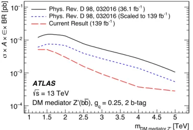
The b-tagged analysis benefits from substantial improvements in the b-jet identification algorithm and associated systematic uncertainties compared with the previous ATLAS result in Ref. [13]. The current and previous expected 95% CL upper limits on the cross-section times branching ratio times acceptance times b-tagging efficiency are shown in Figure9as a function of the Z0mass in the DM benchmark model.
1.5 2 2.5 3 3.5 4 4.5 5 [TeV] DM Mediator Z’ m 0 0.1 0.2 0.3 0.4 0.5 q g ATLAS -1 =13 TeV, 139 fb s 95% CL upper limits σ 1-2 ± Expected Observed
Figure 5: The upper limits on the DM mediator Z0signal at 95% CL from the inclusive category, with the selection described in the text and summarised in Table1. The 95% CL upper limits are set on the universal quark coupling gq as a function of the Z0mass. The observed limits (solid) and expected limits (dashed) with ±1σ and ±2σ uncertainty bands are shown.
1.5 2 2.5 3 3.5 4 4.5 5 [TeV] b* m 4 − 10 3 − 10 2 − 10 1 − 10 1 BR [pb] × ∈ × A × σ Theory Observed 95% CL Expected 95% CL σ 1 ± σ 2 ± ATLAS -1 = 13 TeV, 139 fb s 1 b-tag ≥ b*,
Figure 6: The 95% CL upper limit on the cross-section times acceptance times b-tagging efficiency times branching ratio as a function of the mass of the b∗signal. The expected limit and corresponding ±1σ and ±2σ uncertainty bands are also shown. These exclusion limits are obtained using the 1b category, with the selection described in the text and summarised in Table1.
1.5 2 2.5 3 3.5 4 4.5 5 [TeV] DM mediator Z' m 5 − 10 4 − 10 3 − 10 2 − 10 1 − 10 BR [pb] × ∈ × A × σ Theory Observed 95% CL Expected 95% CL σ 1 ± σ 2 ± ATLAS -1 = 13 TeV, 139 fb s = 0.25 q ), g b DM mediator Z'(b 2 b-tag (a) 1.5 2 2.5 3 3.5 4 [TeV] SSM Z' m 4 − 10 3 − 10 2 − 10 1 − 10 BR [pb] × ∈ × A × σ Theory Observed 95% CL Expected 95% CL σ 1 ± σ 2 ± ATLAS -1 = 13 TeV, 139 fb s ), 2 b-tag b SSM Z'(b (b) 1.5 2 2.5 3 3.5 4 4.5 5 [TeV] G m 5 − 10 4 − 10 3 − 10 2 − 10 1 − 10 BR [pb] × ∈ × A × σ Theory Observed 95% CL Expected 95% CL σ 1 ± σ 2 ± ATLAS -1 = 13 TeV, 139 fb s = 0.2, 2 b-tag PL M ), k/ b G(b (c)
Figure 7: The 95% CL upper limit on the cross-section times acceptance times b-tagging efficiency times branching ratio as a function of the signal mass in the (a) DM mediator Z0with gq= 0.25, (b) SSM Z
0
and (c) graviton with k/MPL= 0.2 models. The expected limit and corresponding ±1σ and ±2σ uncertainty bands are also shown. These exclusion limits are obtained using the 2b category, with the selection described in the text and summarised in Table1.
1 2 3 4 5 6 7 [TeV] X m 4 − 10 3 − 10 2 − 10 1 − 10 BR [pb] × A × σ = 0% X / m X σ = 3% X / m X σ = 5% X / m X σ = 7% X / m X σ = 10% X / m X σ = 15% X / m X σ = 0% X / m X σ Exp. 95% CL upper limit for Obs. 95% CL upper limit for:
ATLAS
-1
= 13 TeV, 139 fb s
Gaussian signals, inclusive
(a) 1 1.5 2 2.5 3 3.5 4 4.5 5 [TeV] X m 4 − 10 3 − 10 2 − 10 1 − 10 BR [pb] × ∈ × A × σ = 0% X / m X σ = 3% X / m X σ = 5% X / m X σ = 7% X / m X σ = 10% X / m X σ = 15% X / m X σ = 0% X / m X σ Exp. 95% CL upper limit for Obs. 95% CL upper limit for:
ATLAS -1 = 13 TeV, 139 fb s 1 b-tag ≥ Gaussian signals, (b) 1 1.5 2 2.5 3 3.5 4 4.5 [TeV] X m 5 − 10 4 − 10 3 − 10 2 − 10 BR [pb] × ∈ × A × σ = 0% X / m X σ = 3% X / m X σ = 5% X / m X σ = 7% X / m X σ = 10% X / m X σ = 15% X / m X σ = 0% X / m X σ Exp. 95% CL upper limit for Obs. 95% CL upper limit for:
ATLAS
-1
= 13 TeV, 139 fb s
Gaussian signals, 2 b-tag
(c)
Figure 8: The 95% CL upper limit on the cross-section times kinematic acceptance times branching ratio for resonances with a generic Gaussian shape, as a function of the Gaussian mean mass mXin the (a) inclusive, (b) 1b and (c) 2b categories. For the limits with one or two b-jets the b-tagging efficiency is included. Different widths, from 0% up to 15% of the signal mass, are considered. Gaussian-shape signals with 0% widths correspond to signal widths smaller than the experimental resolution. For a Gaussian-shaped signal with a relative width of 15%, the limits are truncated at high mass when the broad signal starts to overlap the upper end of the mjjspectrum.
A statistical scaling of the expected upper limits from the previous result (36.1 fb−1) to the current dataset of 139 fb−1is also shown, assuming no change to the previous analysis strategy or its uncertainties. A factor of up to 3.5 improvement beyond that expected from the increase of integrated luminosity in the expected upper limits is observed across the range of masses investigated. The upper limit of the previous result was obtained with the Bayesian method of Ref. [67] and with a looser b-tagging requirement.
[TeV] DM mediator Z’ m 1 1.5 2 2.5 3 3.5 4 4.5 5 BR [pb] × ∈ × A × σ 4 − 10 3 − 10 2 − 10 1 − 10 Phys. Rev. D 98, 032016 (36.1 fb-1 ) ) -1
Phys. Rev. D 98, 032016 (Scaled to 139 fb ) -1 Current Result (139 fb ATLAS = 13 TeV s = 0.25, 2 b-tag q ), g b DM mediator Z’(b
Figure 9: The expected 95% CL upper limits on the cross-section times acceptance times b-tagging efficiency times branching ratio as a function of the DM mediator Z0mass for the current and previous iterations of the analysis. The upper limit of the previous result was obtained with the Bayesian method of Ref. [67] and is also shown scaled to the 139 fb−1integrated luminosity of the current result to illustrate the effect of the analysis improvements. The current b-tagging requirement is tighter than the previous one for high-pTjets, resulting in a data sample with limited size for mjjabove 4 TeV. The background rejection, instead, has improved significantly across the entire mjjspectrum inspected by the analysis.
8 Conclusion
A search for new resonances decaying into a pair of jets has been performed with dijet events using 139 fb−1 of proton–proton collisions recorded at
√
s= 13 TeV with the ATLAS detector at the Large Hadron Collider between 2015 and 2018. The invariant mass spectra of the two highest-momentum jets are analysed inclusively, and with at least one or exactly two jets identified as b-jets. No significant excess is observed above the data-driven estimates of the smoothly falling distributions predicted by the Standard Model. Constraints on various signal models are derived and presented together with model-independent limits on Gaussian-shaped signals. For example, excited quarks q∗with masses below 6.7 TeV are excluded at 95% CL. For the SSM Z0model, Z0masses below 2.7 TeV are excluded at 95% CL. The analysis with b-tagging benefits from substantial improvements in the b-jet identification algorithm at high transverse momentum, resulting in an improvement in sensitivity beyond that expected from the integrated luminosity increase.
Acknowledgements
We thank CERN for the very successful operation of the LHC, as well as the support staff from our institutions without whom ATLAS could not be operated efficiently.
We acknowledge the support of ANPCyT, Argentina; YerPhI, Armenia; ARC, Australia; BMWFW and FWF, Austria; ANAS, Azerbaijan; SSTC, Belarus; CNPq and FAPESP, Brazil; NSERC, NRC and CFI, Canada; CERN; CONICYT, Chile; CAS, MOST and NSFC, China; COLCIENCIAS, Colombia; MSMT CR, MPO CR and VSC CR, Czech Republic; DNRF and DNSRC, Denmark; IN2P3-CNRS and CEA-DRF/IRFU, France; SRNSFG, Georgia; BMBF, HGF and MPG, Germany; GSRT, Greece; RGC and Hong Kong SAR, China; ISF and Benoziyo Center, Israel; INFN, Italy; MEXT and JSPS, Japan; CNRST, Morocco; NWO, Netherlands; RCN, Norway; MNiSW and NCN, Poland; FCT, Portugal; MNE/IFA, Romania; MES of Russia and NRC KI, Russia Federation; JINR; MESTD, Serbia; MSSR, Slovakia; ARRS and MIZŠ, Slovenia; DST/NRF, South Africa; MINECO, Spain; SRC and Wallenberg Foundation, Sweden; SERI, SNSF and Cantons of Bern and Geneva, Switzerland; MOST, Taiwan; TAEK, Turkey; STFC, United Kingdom; DOE and NSF, United States of America. In addition, individual groups and members have received support from BCKDF, CANARIE, Compute Canada and CRC, Canada; ERC, ERDF, Horizon 2020, Marie Skłodowska-Curie Actions and COST, European Union; Investissements d’Avenir Labex, Investissements d’Avenir Idex and ANR, France; DFG and AvH Foundation, Germany; Herakleitos, Thales and Aristeia programmes co-financed by EU-ESF and the Greek NSRF, Greece; BSF-NSF and GIF, Israel; CERCA Programme Generalitat de Catalunya and PROMETEO Programme Generalitat Valenciana, Spain; Göran Gustafssons Stiftelse, Sweden; The Royal Society and Leverhulme Trust, United Kingdom. The crucial computing support from all WLCG partners is acknowledged gratefully, in particular from CERN, the ATLAS Tier-1 facilities at TRIUMF (Canada), NDGF (Denmark, Norway, Sweden), CC-IN2P3 (France), KIT/GridKA (Germany), INFN-CNAF (Italy), NL-T1 (Netherlands), PIC (Spain), ASGC (Taiwan), RAL (UK) and BNL (USA), the Tier-2 facilities worldwide and large non-WLCG resource providers. Major contributors of computing resources are listed in Ref. [68].
References
[1] UA1 Collaboration, Two-jet mass distributions at the CERN proton-antiproton collider,Phys. Lett. B 209 (1988) 127.
[2] UA2 Collaboration, A Search for new intermediate vector mesons and excited quarks decaying to two jets at the CERN ¯pp collider,Nucl. Phys. B 400 (1993) 3.
[3] CDF Collaboration, Search for new particles decaying into dijets in proton-antiproton collisions at√ s = 1.96 TeV,Phys. Rev. D 79 (2009) 112002, arXiv:0812.4036 [hep-ex].
[4] D0 Collaboration, Measurement of Dijet Angular Distributions at √
s= 1.96 TeV and Searches for Quark Compositeness and Extra Spatial Dimensions,Phys. Rev. Lett. 103 (2009) 191803, arXiv: 0906.4819 [hep-ex].
[5] ATLAS Collaboration, Search for new phenomena in dijet events using 37 fb−1of pp collision data collected at
√
s = 13 TeV with the ATLAS detector,Phys. Rev. D 96 (2017) 052004, arXiv: 1703.09127 [hep-ex].
[6] CMS Collaboration, Search for narrow and broad dijet resonances in proton–proton collisions at√ s = 13 TeV and constraints on dark matter mediators and other new particles,JHEP 08 (2018) 130, arXiv:1806.00843 [hep-ex].
[7] ATLAS Collaboration, Search for Low-Mass Dijet Resonances Using Trigger-Level Jets with the ATLAS Detector in pp Collisions at
√
s = 13 TeV, Phys. Rev. Lett. 121 (2018) 081801, arXiv: 1804.03496 [hep-ex].
[8] ATLAS Collaboration, Search for low-mass resonances decaying into two jets and produced in association with a photon using pp collisions at
√
s = 13 TeV with the ATLAS detector,Phys. Lett. B
795 (2019) 56, arXiv:1901.10917 [hep-ex].
[9] ATLAS Collaboration, Search for light resonances decaying to boosted quark pairs and produced in association with a photon or a jet in proton–proton collisions at
√
s= 13 TeV with the ATLAS detector,Phys. Lett. B 788 (2019) 316, arXiv:1801.08769 [hep-ex].
[10] CMS Collaboration, Search for low mass vector resonances decaying to quark–antiquark pairs in proton–proton collisions at
√
s = 13 TeV,Phys. Rev. Lett. 119 (2017) 111802, arXiv:1705.10532 [hep-ex].
[11] CMS Collaboration, Search for low mass vector resonances decaying into quark–antiquark pairs in proton–proton collisions at
√
s= 13 TeV,JHEP 01 (2018) 097, arXiv:1710.00159 [hep-ex]. [12] CMS Collaboration, Search for low-mass resonances decaying into bottom quark–antiquark pairs
in proton–proton collisions at √
s = 13 TeV,Phys. Rev. D 99 (2019) 012005, arXiv:1810.11822 [hep-ex].
[13] ATLAS Collaboration, Search for resonances in the mass distribution of jet pairs with one or two jets identified as b-jets in proton–proton collisions at
√
s = 13 TeV with the ATLAS detector,Phys. Rev. D 98 (2018) 032016, arXiv:1805.09299 [hep-ex].
[14] CMS Collaboration, Search for Narrow Resonances in the b-Tagged Dijet Mass Spectrum in Proton–Proton Collisions at
√
s= 8 TeV,Phys. Rev. Lett. 120 (2018) 201801, arXiv:1802.06149 [hep-ex].
[15] U. Baur, I. Hinchliffe and D. Zeppenfeld, Excited quark production at hadron colliders,Int. J. Mod. Phys. A 02 (1987) 1285.
[16] U. Baur, M. Spira and P. Zerwas, Excited-quark and -lepton production at hadron colliders,Phys. Rev. D 42 (1990) 815.
[17] P. Langacker, The physics of heavy Z’ gauge bosons, Rev. Mod. Phys. 81 (2009) 1199, arXiv: 0801.1345 [hep-ph].
[18] E. Eichten, I. Hinchliffe, K. Lane and C. Quigg, Supercollider physics,Rev. Mod. Phys. 56 (1984) 579, Erratum:Rev. Mod. Phys. 58 (1986) 1065.
[19] G. Altarelli, B. Mele and M. Ruiz-Altaba, Searching for new heavy vector bosons in p ¯p colliders,Z. Phys. C 45 (1989) 109, Erratum:Z. Phys. C 47 (1990) 676.
[20] M. V. Chizhov and G. Dvali, Origin and phenomenology of weak-doublet spin-1 bosons,Phys. Lett. B 703 (2011) 593, arXiv:0908.0924 [hep-ph].
[21] M. V. Chizhov, V. A. Bednyakov and J. A. Budagov, A unique signal of excited bosons in dijet data from pp-collisions,Phys. Atom. Nucl. 75 (2012) 90, arXiv:1010.2648 [hep-ph].
[22] J. Abdallah et al., Simplified models for dark matter searches at the LHC,Phys. Dark Universe 9 (2015) 8, arXiv:1506.03116 [hep-ph].
[23] M. Fairbairn, J. Heal, F. Kahlhoefer and P. Tunney, Constraints on Z’ models from LHC dijet searches and implications for dark matter,JHEP 09 (2016) 018, arXiv:1605.07940 [hep-ph].
[24] D. Abercrombie et al., Dark Matter Benchmark Models for Early LHC Run-2 Searches: Report of the ATLAS/CMS Dark Matter Forum, (2015), arXiv:1507.00966 [hep-ex].
[25] D. Gingrich, Quantum black holes with charge, colour and spin at the LHC, J. Phys. G 37 (2010) 105008, arXiv:0912.0826 [hep-ph].
[26] X. Calmet, W. Gong and S. Hsu, Colorful quantum black holes at the LHC,Phys. Lett. B 668 (2008) 20, arXiv:0806.4605 [hep-ph].
[27] L. Randall and R. Sundrum, Large Mass Hierarchy from a Small Extra Dimension,Phys. Rev. Lett.
83 (1999) 3370, arXiv:hep-ph/9905221.
[28] B. C. Allanach et al., Exploring Small Extra Dimensions at the Large Hadron Collider,JHEP 12 (2002) 039, arXiv:hep-ph/0211205.
[29] ATLAS Collaboration, Search for new phenomena in the dijet mass distribution using pp collision data at
√
s = 8 TeV with the ATLAS detector,Phys. Rev. D 91 (2015) 052007, arXiv:1407.1376 [hep-ex].
[30] ATLAS Collaboration, The ATLAS Experiment at the CERN Large Hadron Collider,JINST 3 (2008) S08003.
[31] ATLAS Collaboration, ATLAS Insertable B-Layer Technical Design Report, ATLAS-TDR-19, 2010, url:https://cds.cern.ch/record/1291633.
[32] B. Abbott et al., Production and integration of the ATLAS Insertable B-Layer,JINST 13 (2018) T05008, arXiv:1803.00844 [physics.ins-det].
[33] ATLAS Collaboration, Performance of the ATLAS trigger system in 2015, Eur. Phys. J. C 77 (2017) 317, arXiv:1611.09661 [hep-ex].
[34] R. D. Ball et al., Parton distributions with LHC data, Nucl. Phys. B 867 (2013) 244, arXiv: 1207.1303 [hep-ph].
[36] T. Sjöstrand, S. Mrenna and P. Z. Skands, A brief introduction to PYTHIA 8.1, Comput. Phys. Commun. 178 (2008) 852, arXiv:0710.3820 [hep-ph].
[37] Z. Nagy, Three Jet Cross Sections in Hadron-Hadron collisions at Next-To-Leading Order,Phys. Rev. Lett. 88 (2002) 122003, arXiv:hep-ph/0110315.
[38] Z. Nagy, Next-to-leading order calculation of three jet observables in hadron hadron collision,Phys. Rev. D 68 (2003) 094002, arXiv:hep-ph/0307268.
[39] S. Catani and M. H. Seymour, A general algorithm for calculating jet cross-sections in NLO QCD, Nucl. Phys. B 485 (1997) 291, arXiv:hep-ph/9605323, Erratum:Nucl. Phys. B 510, 503(1998). [40] J. Alwall et al., The automated computation of tree-level and next-to-leading order differential cross sections, and their matching to parton shower simulations,JHEP 07 (2014) 079, arXiv:1405.0301 [hep-ph].
[41] A. Belyaev, N. D. Christensen and A. Pukhov, CalcHEP 3.4 for collider physics within and beyond the Standard Model,Comput. Phys. Commun. 184 (2013) 1729, arXiv:1207.6082 [hep-ph]. [42] N. Arkani-Hamed, S. Dimopoulos and G. Dvali, The hierarchy problem and new dimensions at a
millimeter,Phys. Lett. B 429 (1998) 263, arXiv:hep-ph/9803315.
[43] D.-C. Dai et al., BlackMax: A black-hole event generator with rotation, recoil, split branes, and brane tension,Phys. Rev. D 77 (2008) 076007, arXiv:0711.3012 [hep-ph].
[44] J. Pumplin et al., New Generation of Parton Distributions with Uncertainties from Global QCD Analysis,JHEP 07 (2002) 012, arXiv:hep-ph/0201195.
[45] ATLAS Collaboration, The ATLAS Simulation Infrastructure,Eur. Phys. J. C 70 (2010) 823, arXiv: 1005.4568 [physics.ins-det].
[46] S. Agostinelli et al., Geant4 – a simulation toolkit,Nucl. Instrum. Meth. A 506 (2003) 250.
[47] ATLAS Collaboration, The simulation principle and performance of the ATLAS fast calorimeter simulation FastCaloSim, ATL-PHYS-PUB-2010-013, 2010, url: https : / / cds . cern . ch / record/1300517.
[48] D. J. Lange, The EvtGen particle decay simulation package,Nucl. Instrum. Meth. A 462 (2001) 152.
[49] A. D. Martin, W. Stirling, R. Thorne and G. Watt, Parton distributions for the LHC,Eur. Phys. J. C
63 (2009) 189, arXiv:0901.0002 [hep-ph].
[50] ATLAS Collaboration, The Pythia 8 A3 tune description of ATLAS minimum bias and inelastic measurements incorporating the Donnachie–Landshoff diffractive model, ATL-PHYS-PUB-2016-017, 2016, url:https://cds.cern.ch/record/2206965.
[51] ATLAS Collaboration, Luminosity determination in pp collisions at √
s= 13 TeV using the ATLAS detector at the LHC, ATLAS-CONF-2019-021, 2019, url:https://cds.cern.ch/record/ 2677054.
[52] G. Avoni et al., The new LUCID-2 detector for luminosity measurement and monitoring in ATLAS, JINST 13 (2018) P07017.
[53] ATLAS Collaboration, Topological cell clustering in the ATLAS calorimeters and its performance in LHC Run 1,Eur. Phys. J. C 77 (2017) 490, arXiv:1603.02934 [hep-ex].
[54] M. Cacciari, G. P. Salam and G. Soyez, The anti-ktjet clustering algorithm,JHEP 04 (2008) 063, arXiv:0802.1189 [hep-ph].
[55] M. Cacciari, G. P. Salam and G. Soyez, FastJet user manual,Eur. Phys. J. C 72 (2012) 1896, arXiv: 1111.6097 [hep-ph].
[56] ATLAS Collaboration, Jet energy scale measurements and their systematic uncertainties in proton– proton collisions at
√
s= 13 TeV with the ATLAS detector,Phys. Rev. D 96 (2017) 072002, arXiv: 1703.09665 [hep-ex].
[57] ATLAS Collaboration, Selection of jets produced in 13 TeV proton–proton collisions with the ATLAS detector, ATLAS-CONF-2015-029, 2015, url:https://cds.cern.ch/record/2037702. [58] ATLAS Collaboration, Identification of Jets Containing b-Hadrons with Recurrent Neural Networks
at the ATLAS Experiment, ATL-PHYS-PUB-2017-003, 2017, url: https://cds.cern.ch/ record/2255226.
[59] ATLAS Collaboration, Optimisation and performance studies of the ATLAS b-tagging algorithms for the 2017-18 LHC run, ATL-PHYS-PUB-2017-013, 2017, url: https://cds.cern.ch/ record/2273281.
[60] ATLAS Collaboration, ATLAS b-jet identification performance and efficiency measurement with t ¯t events in pp collisions at √s = 13 TeV, Eur. Phys. J. C 79 (2019) 970, arXiv: 1907.05120 [hep-ex].
[61] CDF Collaboration, Global search for new physics with 2.0 fb−1 at CDF, Phys. Rev. D 79 (2009) 011101, arXiv:0809.3781 [hep-ex].
[62] G. Choudalakis, On hypothesis testing, trials factor, hypertests and the BumpHunter, 2011, arXiv: 1101.0390 [physics.data-an].
[63] E. Gross and O. Vitells, Trial factors for the look elsewhere effect in high energy physics,Eur. Phys. J. C 70 (2010) 525, arXiv:1005.1891 [hep-ex].
[64] M. Baak et al., HistFitter software framework for statistical data analysis, Eur. Phys. J. C 75 (2015) 153, arXiv:1410.1280 [hep-ex].
[65] A. L. Read, Presentation of search results: the C LStechnique,J. Phys. G 28 (2002) 2693.
[66] G. Cowan, K. Cranmer, E. Gross and O. Vitells, Asymptotic formulae for likelihood-based tests of new physics,Eur. Phys. J. C 71 (2011) 1554, arXiv:1007.1727 [physics.data-an], Erratum: Eur. Phys. J. C 73 (2013) 2501.
[67] A. Caldwell, D. Kollar and K. Kroninger, BAT – The Bayesian Analysis Toolkit, Comput. Phys. Commun. 180 (2009) 2197, arXiv:0808.2552 [physics.data-an].
[68] ATLAS Collaboration, ATLAS Computing Acknowledgements, ATL-SOFT-PUB-2020-001, url: https://cds.cern.ch/record/2717821.
The ATLAS Collaboration
G. Aad102, B. Abbott129, D.C. Abbott103, A. Abed Abud71a,71b, K. Abeling53, D.K. Abhayasinghe94, S.H. Abidi167, O.S. AbouZeid40, N.L. Abraham156, H. Abramowicz161, H. Abreu160, Y. Abulaiti6, B.S. Acharya67a,67b,n, B. Achkar53, S. Adachi163, L. Adam100, C. Adam Bourdarios5, L. Adamczyk84a, L. Adamek167, J. Adelman121, M. Adersberger114, A. Adiguzel12c, S. Adorni54, T. Adye144,
A.A. Affolder146, Y. Afik160, C. Agapopoulou65, M.N. Agaras38, A. Aggarwal119, C. Agheorghiesei27c, J.A. Aguilar-Saavedra140f,140a,ag, F. Ahmadov80, W.S. Ahmed104, X. Ai18, G. Aielli74a,74b, S. Akatsuka86, T.P.A. Åkesson97, E. Akilli54, A.V. Akimov111, K. Al Khoury65, G.L. Alberghi23b,23a, J. Albert176, M.J. Alconada Verzini161, S. Alderweireldt36, M. Aleksa36, I.N. Aleksandrov80, C. Alexa27b,
T. Alexopoulos10, A. Alfonsi120, F. Alfonsi23b,23a, M. Alhroob129, B. Ali142, M. Aliev166, G. Alimonti69a, S.P. Alkire148, C. Allaire65, B.M.M. Allbrooke156, B.W. Allen132, P.P. Allport21, A. Aloisio70a,70b, A. Alonso40, F. Alonso89, C. Alpigiani148, A.A. Alshehri57, M. Alvarez Estevez99, D. Álvarez Piqueras174, M.G. Alviggi70a,70b, Y. Amaral Coutinho81b, A. Ambler104, L. Ambroz135, C. Amelung26, D. Amidei106, S.P. Amor Dos Santos140a, S. Amoroso46, C.S. Amrouche54, F. An79, C. Anastopoulos149, N. Andari145, T. Andeen11, C.F. Anders61b, J.K. Anders20, A. Andreazza69a,69b, V. Andrei61a, C.R. Anelli176,
S. Angelidakis38, A. Angerami39, A.V. Anisenkov122b,122a, A. Annovi72a, C. Antel54, M.T. Anthony149, E. Antipov130, M. Antonelli51, D.J.A. Antrim171, F. Anulli73a, M. Aoki82, J.A. Aparisi Pozo174, L. Aperio Bella15a, J.P. Araque140a, V. Araujo Ferraz81b, R. Araujo Pereira81b, C. Arcangeletti51, A.T.H. Arce49, F.A. Arduh89, J-F. Arguin110, S. Argyropoulos78, J.-H. Arling46, A.J. Armbruster36, A. Armstrong171, O. Arnaez167, H. Arnold120, Z.P. Arrubarrena Tame114, G. Artoni135, S. Artz100, S. Asai163, N. Asbah59, E.M. Asimakopoulou172, L. Asquith156, J. Assahsah35d, K. Assamagan29, R. Astalos28a, R.J. Atkin33a, M. Atkinson173, N.B. Atlay19, H. Atmani65, K. Augsten142, G. Avolio36, R. Avramidou60a, M.K. Ayoub15a, A.M. Azoulay168b, G. Azuelos110,as, H. Bachacou145, K. Bachas68a,68b, M. Backes135, F. Backman45a,45b, P. Bagnaia73a,73b, M. Bahmani85, H. Bahrasemani152, A.J. Bailey174, V.R. Bailey173, J.T. Baines144, M. Bajic40, C. Bakalis10, O.K. Baker183, P.J. Bakker120, D. Bakshi Gupta8, S. Balaji157, E.M. Baldin122b,122a, P. Balek180, F. Balli145, W.K. Balunas135, J. Balz100, E. Banas85, A. Bandyopadhyay24, Sw. Banerjee181,i, A.A.E. Bannoura182, L. Barak161, W.M. Barbe38,
E.L. Barberio105, D. Barberis55b,55a, M. Barbero102, G. Barbour95, T. Barillari115, M-S. Barisits36, J. Barkeloo132, T. Barklow153, R. Barnea160, S.L. Barnes60c, B.M. Barnett144, R.M. Barnett18, Z. Barnovska-Blenessy60a, A. Baroncelli60a, G. Barone29, A.J. Barr135, L. Barranco Navarro45a,45b, F. Barreiro99, J. Barreiro Guimarães da Costa15a, S. Barsov138, R. Bartoldus153, G. Bartolini102, A.E. Barton90, P. Bartos28a, A. Basalaev46, A. Basan100, A. Bassalat65,an, M.J. Basso167, R.L. Bates57, S. Batlamous35e, J.R. Batley32, B. Batool151, M. Battaglia146, M. Bauce73a,73b, F. Bauer145, K.T. Bauer171, H.S. Bawa31,l, J.B. Beacham49, T. Beau136, P.H. Beauchemin170, F. Becherer52, P. Bechtle24, H.C. Beck53, H.P. Beck20,r, K. Becker52, M. Becker100, C. Becot46, A. Beddall12d, A.J. Beddall12a, V.A. Bednyakov80, M. Bedognetti120, C.P. Bee155, T.A. Beermann182, M. Begalli81b, M. Begel29, A. Behera155, J.K. Behr46, F. Beisiegel24, A.S. Bell95, G. Bella161, L. Bellagamba23b, A. Bellerive34, P. Bellos9,
K. Beloborodov122b,122a, K. Belotskiy112, N.L. Belyaev112, D. Benchekroun35a, N. Benekos10,
Y. Benhammou161, D.P. Benjamin6, M. Benoit54, J.R. Bensinger26, S. Bentvelsen120, L. Beresford135, M. Beretta51, D. Berge46, E. Bergeaas Kuutmann172, N. Berger5, B. Bergmann142, L.J. Bergsten26, J. Beringer18, S. Berlendis7, G. Bernardi136, C. Bernius153, F.U. Bernlochner24, T. Berry94, P. Berta100, C. Bertella15a, I.A. Bertram90, O. Bessidskaia Bylund182, N. Besson145, A. Bethani101, S. Bethke115, A. Betti42, A.J. Bevan93, J. Beyer115, D.S. Bhattacharya177, P. Bhattarai26, R. Bi139, R.M. Bianchi139, O. Biebel114, D. Biedermann19, R. Bielski36, K. Bierwagen100, N.V. Biesuz72a,72b, M. Biglietti75a, T.R.V. Billoud110, M. Bindi53, A. Bingul12d, C. Bini73a,73b, S. Biondi23b,23a, M. Birman180, T. Bisanz53,
J.P. Biswal161, D. Biswas181,i, A. Bitadze101, C. Bittrich48, K. Bjørke134, K.M. Black25, T. Blazek28a, I. Bloch46, C. Blocker26, A. Blue57, U. Blumenschein93, G.J. Bobbink120, V.S. Bobrovnikov122b,122a, S.S. Bocchetta97, A. Bocci49, D. Boerner46, D. Bogavac14, A.G. Bogdanchikov122b,122a, C. Bohm45a, V. Boisvert94, P. Bokan53,172,53, T. Bold84a, A.S. Boldyrev113, A.E. Bolz61b, M. Bomben136, M. Bona93, J.S. Bonilla132, M. Boonekamp145, C.D. Booth94, H.M. Borecka-Bielska91, A. Borisov123, G. Borissov90, J. Bortfeldt36, D. Bortoletto135, D. Boscherini23b, M. Bosman14, J.D. Bossio Sola104, K. Bouaouda35a, J. Boudreau139, E.V. Bouhova-Thacker90, D. Boumediene38, S.K. Boutle57, A. Boveia127, J. Boyd36, D. Boye33c,ao, I.R. Boyko80, A.J. Bozson94, J. Bracinik21, N. Brahimi102, G. Brandt182, O. Brandt32, F. Braren46, B. Brau103, J.E. Brau132, W.D. Breaden Madden57, K. Brendlinger46, L. Brenner46,
R. Brenner172, S. Bressler180, B. Brickwedde100, D.L. Briglin21, D. Britton57, D. Britzger115, I. Brock24, R. Brock107, G. Brooijmans39, W.K. Brooks147d, E. Brost121, J.H Broughton21,
P.A. Bruckman de Renstrom85, D. Bruncko28b, A. Bruni23b, G. Bruni23b, L.S. Bruni120, S. Bruno74a,74b, M. Bruschi23b, N. Bruscino73a,73b, P. Bryant37, L. Bryngemark97, T. Buanes17, Q. Buat36, P. Buchholz151, A.G. Buckley57, I.A. Budagov80, M.K. Bugge134, F. Bührer52, O. Bulekov112, T.J. Burch121, S. Burdin91, C.D. Burgard120, A.M. Burger130, B. Burghgrave8, J.T.P. Burr46, C.D. Burton11, J.C. Burzynski103, V. Büscher100, E. Buschmann53, P.J. Bussey57, J.M. Butler25, C.M. Buttar57, J.M. Butterworth95, P. Butti36, W. Buttinger36, C.J. Buxo Vazquez107, A. Buzatu158, A.R. Buzykaev122b,122a, G. Cabras23b,23a,
S. Cabrera Urbán174, D. Caforio56, H. Cai173, V.M.M. Cairo153, O. Cakir4a, N. Calace36, P. Calafiura18, A. Calandri102, G. Calderini136, P. Calfayan66, G. Callea57, L.P. Caloba81b, A. Caltabiano74a,74b, S. Calvente Lopez99, D. Calvet38, S. Calvet38, T.P. Calvet155, M. Calvetti72a,72b, R. Camacho Toro136, S. Camarda36, D. Camarero Munoz99, P. Camarri74a,74b, D. Cameron134, R. Caminal Armadans103, C. Camincher36, S. Campana36, M. Campanelli95, A. Camplani40, A. Campoverde151, V. Canale70a,70b, A. Canesse104, M. Cano Bret60c, J. Cantero130, T. Cao161, Y. Cao173, M.D.M. Capeans Garrido36, M. Capua41b,41a, R. Cardarelli74a, F. Cardillo149, G. Carducci41b,41a, I. Carli143, T. Carli36, G. Carlino70a, B.T. Carlson139, L. Carminati69a,69b, R.M.D. Carney45a,45b, S. Caron119, E. Carquin147d, S. Carrá46, J.W.S. Carter167, M.P. Casado14,e, A.F. Casha167, D.W. Casper171, R. Castelijn120, F.L. Castillo174, V. Castillo Gimenez174, N.F. Castro140a,140e, A. Catinaccio36, J.R. Catmore134, A. Cattai36, V. Cavaliere29, E. Cavallaro14, M. Cavalli-Sforza14, V. Cavasinni72a,72b, E. Celebi12b, F. Ceradini75a,75b,
L. Cerda Alberich174, K. Cerny131, A.S. Cerqueira81a, A. Cerri156, L. Cerrito74a,74b, F. Cerutti18, A. Cervelli23b,23a, S.A. Cetin12b, Z. Chadi35a, D. Chakraborty121, W.S. Chan120, W.Y. Chan91, J.D. Chapman32, B. Chargeishvili159b, D.G. Charlton21, T.P. Charman93, C.C. Chau34, S. Che127, S. Chekanov6, S.V. Chekulaev168a, G.A. Chelkov80,al, M.A. Chelstowska36, B. Chen79, C. Chen60a, C.H. Chen79, H. Chen29, J. Chen60a, J. Chen39, S. Chen137, S.J. Chen15c, X. Chen15b, Y-H. Chen46, H.C. Cheng63a, H.J. Cheng15a, A. Cheplakov80, E. Cheremushkina123, R. Cherkaoui El Moursli35e, E. Cheu7, K. Cheung64, T.J.A. Chevalérias145, L. Chevalier145, V. Chiarella51, G. Chiarelli72a, G. Chiodini68a, A.S. Chisholm21, A. Chitan27b, I. Chiu163, Y.H. Chiu176, M.V. Chizhov80, K. Choi66, A.R. Chomont73a,73b, S. Chouridou162, Y.S. Chow120, M.C. Chu63a, X. Chu15a,15d, J. Chudoba141, A.J. Chuinard104, J.J. Chwastowski85, L. Chytka131, D. Cieri115, K.M. Ciesla85, D. Cinca47, V. Cindro92, I.A. Cioară27b, A. Ciocio18, F. Cirotto70a,70b, Z.H. Citron180,j, M. Citterio69a, D.A. Ciubotaru27b,
B.M. Ciungu167, A. Clark54, M.R. Clark39, P.J. Clark50, C. Clement45a,45b, Y. Coadou102, M. Cobal67a,67c, A. Coccaro55b, J. Cochran79, H. Cohen161, A.E.C. Coimbra36, L. Colasurdo119, B. Cole39, A.P. Colijn120, J. Collot58, P. Conde Muiño140a,140h, S.H. Connell33c, I.A. Connelly57, S. Constantinescu27b,
F. Conventi70a,at, A.M. Cooper-Sarkar135, F. Cormier175, K.J.R. Cormier167, L.D. Corpe95,
M. Corradi73a,73b, E.E. Corrigan97, F. Corriveau104,ae, M.J. Costa174, F. Costanza5, D. Costanzo149, G. Cowan94, J.W. Cowley32, J. Crane101, K. Cranmer125, S.J. Crawley57, R.A. Creager137,