275 Candidates and 149 Validated Planets
Orbiting Bright Stars in K-2 Campaigns 0-10
The MIT Faculty has made this article openly available.
Please share
how this access benefits you. Your story matters.
Citation
Mayo, Andrew W., et al., "275 Candidates and 149 Validated
Planets Orbiting Bright Stars in K-2 Campaigns 0-10."
Astronomical Journal 155, 3 (March 2018): no. 136 doi http://
dx.doi.org/10.3847/1538-3881/AAADFF ©2018 Author(s)
As Published
http://dx.doi.org/10.3847/1538-3881/AAADFF
Publisher
American Astronomical Society
Version
Final published version
Citable link
https://hdl.handle.net/1721.1/124535
Terms of Use
Article is made available in accordance with the publisher's
policy and may be subject to US copyright law. Please refer to the
publisher's site for terms of use.
275 Candidates and 149 Validated Planets Orbiting Bright Stars in
K2 Campaigns 0–10
Andrew W. Mayo1,2,3,20,21 , Andrew Vanderburg3,4,20,22 , David W. Latham3 , Allyson Bieryla3 , Timothy D. Morton5 , Lars A. Buchhave1,2 , Courtney D. Dressing6,7,22 , Charles Beichman8, Perry Berlind3, Michael L. Calkins3 , David R. Ciardi8 , Ian J. M. Crossfield9, Gilbert A. Esquerdo3 , Mark E. Everett10 , Erica J. Gonzales11,20, Lea A. Hirsch6 , Elliott P. Horch12 , Andrew W. Howard13 , Steve B. Howell14 , John Livingston15 , Rahul Patel16 , Erik A. Petigura13,23 ,
Joshua E. Schlieder17, Nicholas J. Scott14 , Clea F. Schumer3, Evan Sinukoff13,18 , Johanna Teske19,24, and Jennifer G. Winters3
1
DTU Space, National Space Institute, Technical University of Denmark, Elektrovej 327, DK-2800 Lyngby, Denmark;awm@space.dtu.dk
2
Centre for Star and Planet Formation, Natural History Museum of Denmark & Niels Bohr Institute, University of Copenhagen, Øster Voldgade 5-7, DK-1350 Copenhagen K., Denmark
3
Harvard–Smithsonian Center for Astrophysics, 60 Garden Street, Cambridge, MA 02138, USA 4
Department of Astronomy, University of Texas at Austin, Austin, TX 76712, USA 5
Department of Astrophysical Sciences, 4 Ivy Lane, Peyton Hall, Princeton University, Princeton, NJ 08544, USA 6
Astronomy Department, University of California, Berkeley, CA 94720, USA 7
Division of Geological & Planetary Sciences, California Institute of Technology, 1200 East California Boulevard MC 150-21, Pasadena, CA 91125 USA 8
NASA Exoplanet Science Institute, California Institute of Technology, Pasadena, CA 91125, USA 9
Department of Physics and Kavli Institute for Astrophysics and Space Research, Massachusetts Institute of Technology, Cambridge, MA 02139, USA 10National Optical Astronomy Observatory, 950 North Cherry Avenue, Tucson, AZ 85719, USA
11
Department of Astronomy and Astrophysics, University of California, Santa Cruz, CA 95064, USA 12
Department of Physics, Southern Connecticut State University, 501 Crescent Street, New Haven, CT 06515, USA 13
Cahill Center for Astrophysics, California Institute of Technology, Pasadena, CA 91125, USA 14
Space Science and Astrobiology Division, NASA Ames Research Center, Moffett Field, CA 94035, USA 15
Department of Astronomy, The University of Tokyo, 7-3-1 Hongo, Bunkyo-ku, Tokyo 113-0033, Japan 16
Infrared Processing and Analysis Center, California Institute of Technology, Pasadena, CA 91125, USA 17
NASA Goddard Space Flight Center, Greenbelt, MD 20771, USA 18
Institute for Astronomy, University of Hawai‘i at Mānoa, Honolulu, HI96822, USA 19
Carnegie Observatories, 813 Santa Barbara Street, Pasadena, CA 91101, USA
Received 2017 December 15; revised 2018 January 18; accepted 2018 January 25; published 2018 March 6
Abstract
Since 2014, NASA’s K2 mission has observed large portions of the ecliptic plane in search of transiting planets and has detected hundreds of planet candidates. With observations planned until at least early 2018, K2 will continue to identify more planet candidates. We present here 275 planet candidates observed during Campaigns 0–10 of the K2 mission that are orbiting stars brighter than 13 mag (in Kepler band) and for which we have obtained high-resolution spectra(R = 44,000). These candidates are analyzed using the vespa package in order to calculate their false-positive probabilities(FPP). We find that 149 candidates are validated with an FPP lower than 0.1%, 39 of which were previously only candidates and 56 of which were previously undetected. The processes of data reduction, candidate identification, and statistical validation are described, and the demographics of the candidates and newly validated planets are explored. We show tentative evidence of a gap in the planet radius distribution of our candidate sample. Comparing our sample to the Kepler candidate sample investigated by Fulton et al., we conclude that more planets are required to quantitatively confirm the gap with K2 candidates or validated planets. This work, in addition to increasing the population of validated K2 planets by nearly 50% and providing new targets for follow-up observations, will also serve as a framework for validating candidates from upcoming K2 campaigns and the Transiting Exoplanet Survey Satellite, expected to launch in 2018.
Key words: methods: data analysis– planets and satellites: detection – techniques: photometric Supporting material: machine-readable tables
1. Introduction
Thefield of exoplanets is relatively young compared to most other disciplines of astronomy: the announcement of the first exoplanet orbiting a star similar to our own was made only in 199525 (Mayor & Queloz 1995). Since then, the field has
expanded rapidly, with several thousand exoplanets having now been discovered. With many upcoming extremely large telescopes, the number of known exoplanets and our under-standing of them will only increase.
One of the most important moments in the history of exoplanet science was the beginning of the Kepler mission (Borucki et al. 2008). Launched in 2009, the Kepler space telescope
observed over 100,000 stars in a single patch of sky for four years in order to look for transits. Kepler has been an overwhelming success. According to the NASA Exoplanet Archive26(accessed 2018 February 14), it is currently responsible for 2341 verified exoplanets, more than every other exoplanet survey combined.
The Astronomical Journal, 155:136 (25pp), 2018 March https://doi.org/10.3847/1538-3881/aaadff
© 2018. The American Astronomical Society. All rights reserved.
20
National Science Foundation Graduate Research Fellow. 21
Fulbright Fellow. 22
NASA Sagan Fellow. 23
NASA Hubble Fellow. 24
Carnegie Origins Fellow, jointly appointed by Carnegie DTM & Carnegie Observatories.
25
The exoplanet 51 Peg b was not fully confirmed to be a planet until the absolute mass was measured by Martins et al.(2015). Moreover, a reported
brown dwarf discovered in 1989 (Latham et al. 1989) may in fact be an
exoplanet, depending on its inclination. 26https://exoplanetarchive.ipac.caltech.edu/
Unfortunately, in 2013 the second of four reaction wheels on the Kepler spacecraft failed, preventing the spacecraft from looking at its designated field and bringing an end to the original mission. Fortunately, a follow-up mission, called K2, was developed that used the spacecraft’s thrusters as a makeshift third reaction wheel (Howell et al. 2014). Unlike
the original Kepler mission, the K2 mission must observe new fields roughly every 83 days.27As a result, K2 observations are
divided into“campaigns”, each corresponding to a field. With every new campaign, K2 observes more bright stars and finds more planets orbiting these stars, so there are new bright targets available for follow-up such as radial velocity (RV) measurements or transmission spectroscopy. K2 has led to the discovery of numerous candidate and confirmed planets (Crossfield et al. 2015; Foreman-Mackey et al. 2015; Montet et al.2015; Vanderburg et al.2015b,2016b; Adams et al.2016; Barros et al. 2016; Crossfield et al. 2016; Schlieder et al.
2016; Sinukoff et al. 2016; Pope et al. 2016; Dressing et al. 2017b; Hirano et al. 2017; Martinez et al. 2017), as
well as to the identification of planets orbiting rare types of stars, including particularly bright nearby dwarf stars(Petigura et al.2015; Vanderburg et al.2016a; Christiansen et al.2017; Crossfield et al. 2017; Niraula et al. 2017; Rodriguez et al. 2017a, 2017b), young, pre-main-sequence stars (Mann
et al. 2016; David et al. 2016), and disintegrating planetary
material transiting a white dwarf(Vanderburg et al.2015a).
Here, we take advantage of the large number of bright stars observed by K2 and present the identification and follow-up of a sample of 275 exoplanet candidates orbiting stars (brighter than 13 mag) in the Kepler bandpass identified from K2 Campaigns 0 through 10. Since the beginning of the K2 mission, we have also obtained spectra for all of our candidates, as well as many high-resolution imaging observations, in order to measure the candidate host stars’ parameters and identify nearby stars (both types of follow-up aid in identification and ruling out of false-positive scenarios). We also attempt to validate28 our candidates with vespa, a statistical validation tool developed by Morton (2012, 2015b), finding 149 to be
validated with a false-positive probability (FPP) lower than 0.1%. Of these newly validated exoplanets, 39 were previously only exoplanet candidates and 56 have not been previously detected. This work will increase the validated K2 planet sample from 212(according to the Mikulski Archive for Space Telescopes29; accessed 2018 February 14) to 307, an increase
of nearly 50%. Similarly, this work increases the K2 candidate sample by∼20%.
In this paper, we describe the identification and analysis of our candidate sample, as well as our validation process and the resulting validated planet sample. Section 2 discusses the process by which we use K2 data to identify exoplanet candidates. Section3describes our ground-based observations of the planet candidate host stars detected by K2. Section 4
explains the analysis of the K2 light curves and the follow-up spectroscopy and high-contrast imaging. Section5details how we use vespa to calculate FPPs for our planet candidates. Section 6 presents the results of our candidate identification, vetting, follow-up observations, and analysis in detail for a single, instructive planet. Then the results for the entire planet candidate sample are similarly presented. In Section 7 we discuss the results of our work, including confirmation of features in the exoplanet population previously identified using data from the original Kepler mission. Finally, we summarize and conclude in Section8.
2. Pixels to Planets
In this section, we first explain how K2 observations are collected, then we describe the process by which systematic errors are removed from K2 data, and finally we discuss the analysis of the systematics-corrected K2 data in order to identify planet candidates.
2.1. K2 Observations
Since 2014, the K2 mission has served as the successor to the original Kepler mission. By observingfields along the ecliptic plane and firing its thrusters approximately once every six hours, the probe can maintain an unstable equilibrium against solar radiation. However, the spacecraft can only point toward a givenfield for roughly 83 days before re-pointing (in order to keep sunlight on the spacecraft panels and out of its telescope). Because of on-board data storage constraints, not all data collected by the CCD array can be retained and transmitted to the ground. As a result, targets must be identified within each campaignfield prior to observation so that non-target data can be discarded and a postage stamp (a small group of pixels) around each target can be saved and transmitted to the ground. In the original Kepler mission, the primary objective was to determine the frequency of Earth-like planets orbiting Sun-like stars (Batalha et al. 2010a). Although some planet search
targets were selected during mission adjustments and others were selected through a Guest Observer (GO) program for secondary science objectives, most targets were selected pre-launch for the primary objective. However, K2 operates in a very different manner. For each K2 campaign, targets are exclusively selected through the GO program, which evaluates observing proposals submitted by the astronomical community for any scientific objective, not just exoplanet-related objec-tives. Ideally, GO proposals have scientifically compelling goals that can be achieved through K2 observations and cannot easily be achieved with other instruments or facilities.
In a typical K2 campaign, the number of targets ranges between 10,000 and 40,000 with long-cadence observations (≈30-minute integration), and about 50–200 with short-cadence observations (≈1-minute integration). Exceptions include C0, which served primarily as a proof-of-concept campaign to show that the K2 mission was viable, and C9,
27
Roughly 75 of those days are devoted to science. 28
The difference between an exoplanet candidate and a validated exoplanet is very important. During the original Kepler mission, an exoplanet candidate was a transit signal that had passed a battery of astrophysical false-positive and instrumental false-alarm tests. In K2, however, the usage is looser; the term is commonly used to refer to any exoplanet signal that a particular team has identified as a possible planet. So long as the reasoning is sound and the results are published, the signal is effectively a candidate. A validated planet is a candidate that has been vetted with follow-up observations and determined quantitatively to be far more likely an exoplanet than a false positive(according to some likelihood threshold). Validated planets, because confidence in their planethood is higher than for a regular candidate, are far more promising targets than planet candidates for follow-up observations, characterization, and eventual confirmation. We note that validation is not the same as confirmation, which is ideally attained through a reliable mass determination. In this work, we are in general not attempting to“confirm” planets. Confirmation is more rigorous than validation, in the same way that validation is more rigorous than candidacy. Confirmation is usually accomplished via the RV method, the TTV method, or, less commonly, methods such as a full photodynamical modeling solution (e.g., Carter et al. 2011) or Doppler tomography (e.g., Zhou
et al.2016).
29
which focused on microlensing targets in the Galactic Bulge. Both C0 and C9 had fewer targets than normal in both long cadence and short cadence. It should also be noted that there are occasional overlaps between campaignfields. Despite fewer new targets, overlaps provide a longer baseline of observations for targets of interest in the overlapping region.
This paper focuses on Campaigns 0 through 10 (excluding Campaign 9). However, the process implemented in this research can easily be extended and applied to additional K2 campaigns.
2.2. K2 Data Reduction
Because of the loss of two reaction wheels, the Kepler telescope is perpetually drifting off target and must be regularly corrected by thruster fires, causing shifts in the pixels that targets fall on. These shifts, coupled with variable sensitivity between pixels on the telescope CCDs and variable amounts of starlight falling inside photometric apertures, lead to systematic variations in the signal from K2 targets, introducing noise into the photometric measurements. Howell et al.(2014) estimated
that raw K2 precision is roughly a factor of 3–4 times worse than the original Kepler precision (depending on stellar magnitude). Fortunately, an understanding of the motion of the Kepler spacecraft allows for modeling and correction of the induced systematic noise. In particular, we rely on the method of systematic correction described by Vanderburg & Johnson (2014, hereafter referred to asVJ14), as well as the updates to
the method described in Vanderburg et al. (2016a, hereafter referred to as V16). We briefly describe here the method
developed byVJ14.
First, 20 different aperture masks were chosen for each target star, 10 circular masks of varying size and 10 masks shaped liked the Kepler pixel response function (PRF) for the target with varying sensitivity cutoffs. These masks were used to perform simple aperture photometry to produce 20 different “raw” light curves. Then the motion of the target star across the CCD was estimated by calculating centroid position for each cadence.30 Next, the recurrent path of the centroid across the CCD between thruster fires was identified. Data collected during thruster fires were identified and removed. Then, for each of the 20 raw light curves produced, low-frequency variations (>1.5 days) were removed with a basis spline, and the relationship between centroid position andflux was fit with a piecewise function. Because the centroid path would shift on timescales longer than 5–10 days, the flux-centroid piecewise function was applied separately to each light-curve segment of 5–10 days. This function was then used to correct the raw data so that low-frequency variations could be recalculated. This process was then repeated iteratively until convergence. Finally, after all 20 raw light curves per star were processed in this way, a “best” aperture was chosen to maximize photometric precision. An example of a light curve before and after the full data reduction procedure can be seen in Figure 1
for the planet host EPIC 212521166. We note that light from any nearby companion star could potentially enter the best aperture mask, which may lead to a diluted transit and an underestimated planet radius (Ciardi et al. 2015; Hirsch
et al. 2017). However, we expected this effect to be small
even when present and therefore did not correct for it.
2.3. Identifying Threshold-crossing Events
After the roll systematics were removed from the photometry according to the method described by VJ14, we conducted a transit search of each K2 target using the method of Vanderburg et al.(2016b). We give a short description of the
transit search process here.
First, low-frequency variations were removed via a basis spline and outliers were removed. Then a box-least-squares (BLS) periodogram (Kovács et al.2002) was calculated over
periods between 2.4 hr and half the length of the campaign. All periodic decreases in brightness with a signal-to-noise ratio (S/N)>9 were investigated. If putative transits lasted longer than 20% of their period, were composed of a single data point, or changed depth by over 50% when the lowest point was removed, the signal was removed and the BLS periodogram recalculated. Any detection passing these tests was deemed a threshold-crossing event (TCE). We identified ∼30,000 TCEs across C0–C10 in this manner.
Each TCE was fit with the Mandel & Agol (2002) transit
model to estimate transit parameters, then the TCE was removed from the light curve, and the BLS periodogram was recalculated. After all TCEs had been identified, they subsequently underwent “triage,” in which each candidate was inspected by eye in order to remove obvious astrophysical false positives and instrumental false alarms from subsequent analysis. TCEs identified as neither type of false signal passed the triage phase and moved on to a“vetting” phase.
2.4. Identifying K2 Candidates
During vetting, we subjected the surviving TCEs to a battery of additional tests to identify astrophysical false positives and instrumental false alarms. Some of these tests were identical or similar to the tests conducted for the Kepler mission, while others are specific to K2 data. For each test we produced a
Figure 1.Example of the K2 systematics reduction process on the light curve of the planet host EPIC 212521166. The blue points show the light curve before correcting for the systematics induced by the roll motion of the Kepler spacecraft, while the yellow points show the same light curve after those systematics have been removed via the data reduction process summarized in Section2.2and documented in Vanderburg & Johnson(2014) and Vanderburg
et al.(2016b). The remaining downward dips in the corrected (yellow) light
curve are transits of a mini-Neptune sized exoplanet, validated in this work and previously confirmed in Osborn et al. (2017).
30
Although it is possible to produce light curves by decorrelating with centroid positions measured from each star, we used the centroids measured from one hand-selected isolated, bright K2 target per campaign, which we found gives better results.
3
diagnostic plot, examples of which are shown in Figures 2–4. Here we describe the tests we conducted in more detail.
1. The times of the in-transit points of a TCE were compared against the position of the Kepler spacecraft at these times, as many instrumental false alarms were composed of data points near the edges of Kepler rolls where the K2 flat field is less well constrained, and our analysis method can leave in systematics. The plots we used to identify these false alarms are shown in Figures2
and 3.
2. We compared the signal of a TCE in light curves produced using multiple different photometric apertures. This test is a powerful way to identify signals caused by instrumental systematics (as these systematics present differently in different photometric apertures), as well as
identifying astrophysical false positives, such as when a candidate transit signal was due to contamination from a nearby star. An example of these tests is shown in Figure3. We note that although this test rules out transits or eclipses originating from a nearby companion, it does not rule out the possibility of light contamination from a nearby companion, which could dilute the observed transit and lead to an underestimation of the planetary radius(Ciardi et al.2015; Hirsch et al. 2017).
3. Individual transits of a TCE were visually inspected, since instrumental false alarms were less likely to have consistent, planet-like transit depths or shapes (see Figure 2). This metric is qualitatively similar to the
“transit patrol” metrics introduced in the DR25 Kepler planet candidate catalog (in particular the Rubble,
Figure 2.Diagnostic plots for EPIC 212521166.01. Left column,first (top) and second rows: K2 light curves without and with low-frequency variations removed, respectively. The low-frequency variations alone are modeled in red in thefirst row, whereas the best-fit transit model is shown in red in the second row. Vertical brown dotted lines denote the regions into which the light curve was separated to correct roll systematics. Left column, third and fourth rows: phase-folded, low-frequency corrected K2 light curves. In the third row, the full light curve is shown(points more than one half-period from the transit are gray), whereas in the fourth row, only the light curve near transit is shown. The red line is the best-fit model, and the blue points are binned data points. Middle column, first and second rows: arclength of centroid position of star vs. brightness, after and before roll systematics correction, respectively. Red points denote in-transit data. In the second row, small orange points denote the roll systematics correction made to the data. Middle column, third row: separate plotting and modeling of odd(left panel) and even (right panel) transits, with orange and blue data points, respectively. The black line is the best-fit model, the horizontal red line denotes the modeled transit depth, and the vertical red line denotes the mid-transit time(this is useful for detecting binary stars with primary and secondary eclipses). Middle column, fourth row: light curve data in and around the expected secondary eclipse time(for zero eccentricity). Blue data points are binned data, the horizontal red line denotes a relative flux=1, and the two vertical red lines denote the expected beginning and end of the secondary eclipse. Right column: individual transits(vertically shifted from one another) with the best-fit model in red and the vertical blue lines denoting the beginning and end of transit.
Marshall, Chases, and Zuma tests; Thompson et al.
2017).
4. Flux-centroid motion, phase variations(possibly caused by relativistic beaming, reflected light, or ellipsoidal effects), differences in depth between odd- and even-numbered transits, and secondary eclipses were all searched for as evidence of astrophysical false positives. Similar tests have been used since the beginning of the Kepler mission (Batalha et al. 2010b). Example
diag-nostic plots for identifying phase variations, the differ-ence between even- and odd-numbered transits, and secondary eclipses near phase 0.5 are shown in Figure2; flux-centroid shift tests are shown in Figure 3. We searched for secondary eclipses at arbitrary phases (not necessarily near phase=0.5) using the model-shift uniqueness test designed by Coughlin et al. (2016). We
show diagnostic plots for the model-shift uniqueness test in Figure4.
5. We searched for astrophysical false-positive scenarios by ephemeris matching. Sometimes the pixels surrounding a target star can be contaminated with a small amount of light from other nearby stars. When those nearby stars are variable themselves (like eclipsing binaries), the varia-bility from the nearby stars can be introduced into the target’s light curve (Coughlin et al.2014). We identified
cases where this happened by searching for planet candidates that have the same period(or integer multiples of the same period) and time of transit as eclipsing binaries observed by K2 using the same criteria as Coughlin et al. (2014). We found no examples of
matched ephemerides due to direct PRF overlap that we had not also identified in our tests with multiple
Figure 3.Diagnostic plots for EPIC 212521166.01. Left column,first (top), second, and third rows: images from the first Digital Sky Survey, the second Digital Sky Survey, and K2, respectively, each with a scale bar near the top and an identical red polygon to show the shape of the photometric aperture chosen for reduction. The K2 image is rotated into the same orientation as the two archival images(north is up). Middle column, top row: multiple panels of uncorrected brightness vs. arclength, chronologically ordered and separated into the divisions in which the roll systematics correction was calculated. In-transit data points are shown in red, orange points denote the brightness correction applied to remove systematics. Middle column, bottom row: variations in the centroid position of the K2 image. In-transit points are red. The discrepancy(in standard deviations) between the mean centroid position in transit and out-of-transit is shown on the right side of the plot. Right column, first row: the K2 light curve near transit as calculated using three differently sized apertures: small mask(top panel), medium mask (middle panel), and large mask (bottom panel), each with the identical best-fit model in red. Aperture-size dependent discrepancies in depth could suggest background contamination from another star. Right column, third row: the K2 image overlaid with the three masks from the previous plot shown(in this figure, the large mask is fully outside the postage stamp and is therefore not visible).
5
photometric apertures, but we did find two instances where candidate transit signals were caused by charge transfer inefficiency along one of the columns of the Kepler detector. We excluded a candidate around EPIC 212435047 caused by contamination from the eclipsing binary EPIC 212409377 located along the same CCD column about 2000 arcsec away, and we excluded a candidate around EPIC 202710713 contaminated by the eclipsing binary EPIC 202685801 located along the same CCD column at a distance of about 300 arcsec.
6. We estimated the S/N of a TCE by taking the difference between the mean baselineflux and the in-transit flux and dividing by the quadrature sum of the standard deviation of the flux in those two regions. We defined the boundaries of the in-transit region in two ways and calculated the S/N for both choices. In one case we used every data point collected between the second and third contact(minus a single long-cadence Kepler exposure on either side). This estimate of S/N could sometimes not be calculated if the transit was grazing. In the other case we used the central 20% of data collected from the first to fourth contact (which could be calculated even if the transit was grazing). Following standard practice from the Kepler mission, if both of these values(or just the latter in
the grazing case) were below 7.1σ, the candidate was excluded (7.1σ is the minimum significance level for a signal to qualify as a TCE in the Kepler Science Pipeline; Jenkins et al. 2010). We only encountered two such
candidates: EPIC 220474074 and EPIC 201289302. Although it is possible to automate diagnostic tests of this type(see, for example, the Robovetter that was designed for the main Kepler mission; Coughlin et al. 2016), we performed
vetting tests 1–4 by eye.
Any TCE surviving all of these vetting stages was promoted to planet candidate (∼1000 were promoted in this way). All candidates orbiting sufficiently bright host stars (see Section 3.1) were then subjected to our validation process.
275 candidates satisfied these requirements and were subjected to validation. Their associated stellar parameters are listed in Table3.
3. Supporting Observations
In this section, we describe the follow-up observations we conducted to better characterize the candidate host stars. These observations are crucial for improving stellar parameters(e.g., Dressing et al.2017a; Mann et al.2017; Martinez et al.2017), Figure 4.Model-shift uniqueness diagnostic plots for EPIC 212521166.01. We cross-correlated the phase-folded light curve of each planet candidate with the best-fitting transit model for the candidate. The two plots in the top row show the cross-correlation function as a function of orbital phase with different scaling on the Y-axis. The tallest peak in the response is the primary transit, and the three vertical lines show the phase of the highest significance putative secondary event (red) , the second-highest significance putative secondary event (orange), and the highest significance upside-down secondary event (blue). The bottom row of plots show the three segments of the light curve surrounding the highest and second-highest significance putative secondary eclipses, and the highest significance upside-down event. Gray and purple data points are unbinned and binned observations, respectively. Comparing the amplitudes of these three events gives an indication of their significance. Here, the two most significant putative secondary eclipses have a similar amplitude to the most significant upside-down event, indicating that they are all likely spurious. Wefind no significant secondary eclipse in the light curve of EPIC 212521166.01.
which in turn can help differentiate between a transiting planet and various false-positive scenarios (i.e., stellar binary config-urations) that might prefer different regions of stellar parameter space. Wefirst discuss high-resolution optical spectroscopy of the planet candidate host stars from the Tillinghast Reflector Echelle Spectrograph (TRES), followed by speckle imaging from the Differential Speckle Survey Instrument (DSSI) and the NASA Exoplanet Star and Speckle Imager (NESSI) at the WIYN telescope,31 the Gemini South telescope, and the Gemini North telescope, and finally, adaptive optics (AO) imaging from Keck Observatory, Palomar Observatory, Gemini South Observatory, Gemini North Observatory, and the Large Binocular Telescope Observatory.
3.1. TRES Observations
All of the spectra used in this work were obtained with TRES, a spectrograph with a resolving power of R=44,000 and one of two spectrographs for the 1.5 m Tillinghast telescope at the Whipple Observatory on Mt. Hopkins in Arizona. We obtained at least one usable TRES spectrum of each of the planet candidate host stars that we consider in this work and that we subject to our validation process (see Section 4.2 for our definition of “usable”). With a few exceptions, we only observed candidates brighter than 13 mag in the Kepler band with TRES because of the lengthy integration time required to collect spectra of stars fainter than this and the difficulty of subsequent follow-up observations (for example, with precise radial velocities) at other facilities. This limitation reduced the number of candidates we considered for validation significantly, from ∼1000 to 275. In the future, observing these fainter candidates, either with TRES or other spectrographs on larger telescopes, could potentially more than double the number of K2 planets for our analysis.
3.2. Speckle Observations
We observed many of our planet candidates with speckle imaging from either the 3.5m WIYN telescope, the Gemini-South 8.1m telescope, or the Gemini-North 8.1m telescope. Together, the three telescopes collected 162 speckle images of 73 stars with DSSI (Horch et al. 2009). DSSI is a
speckle-imaging instrument that travels between different telescopes. For each of the 73 targets, we collected DSSI speckle images at narrowbandfilters centered at 6920 and 8800 Å (at least one of each for every target). These observations were made in 2015 September and October, as well as in 2016 January, April, and June.
Furthermore, 160 speckle images were collected for a distinct sample of 70 stars at the WIYN telescope using NESSI, which is essentially a newer version of the DSSI instrument. For each of the 70 targets, we collected NESSI speckle images at narrowband filters centered at 5620 and 8320Å (at least one of each). These observations were made in 2016 October through November and 2017 March through May. A list of the observed stars can be found in Table1.
3.3. AO Observations
In addition to speckle imaging, we also observed many of our planet candidate host stars with AO imaging.
We collected 47 AO images for 45 stars on the Keck II 10m telescope in K filter with the Near Infra Red Camera 2 (NIRC2); 5 of these stars were also imaged using NIRC2 in J band. All of these observations were made during 2015 April, July, August, and October and in 2016 January and February. We collected 27 AO images for 27 stars on the Palomar 5.1m Hale telescope in K filter with the Palomar High Angular Resolution Observer (PHARO, Hayward et al. 2001); 6 of
these stars were also imaged using PHARO in J band. All of these observations were made during 2015 February, May, and August and in 2016 June, September, and October.
We collected 19 AO images for 18 stars on the Gemini-North 8.1m telescope in K band with the Near InfraRed Imager and spectrograph (NIRI, Hodapp et al. 2003). These
observations were made during 2015 October and November and in 2016 June and October.
We collected a single AO image on the Large Binocular Telescope in Kfilter with the L/M-band mid-infraRed Camera (LMIRCam, Leisenring et al. 2012). This observation was
made in 2015 January.
There was some overlap between instruments; overall, AO images were collected for a total of 80 systems. A list of the observed stars can be found in Table1.
4. Data Analysis
After all of the photometry had been reduced and all of the necessary follow-up observations had been collected, the next step was to analyze the data, calculate relevant parameters, and prepare the results for the validation process. In this section, we explain the process of fitting a model to our reduced light curves(to determine transit parameters and create folded light curves), analyzing our spectra (to calculate stellar parameters), and extracting and reducing data from our high-contrast images (to create contrast curves).
4.1. K2 Light Curves
4.1.1. Simultaneous Fitting of K2 Systematics and Transit Parameters
In Sections 2.2, 2.3, and 2.4, we described the process of correcting K2 photometry for instrumental systematics and exploring the reduced light curves for candidates. After these steps were completed, the planet candidates needed to be more thoroughly characterized. In order to assess transit and orbital parameters, we reproduced the K2 light curves for these planet candidates by rederiving the systematics correction while simultaneously modeling the transits in the light curve. As in our original systematics correction, the light curve was divided
Table 1 High-resolution Imaging
EPIC Filter Instrument
201110617 562 NESSI
201110617 832 NESSI
201111557 562 NESSI
(This table is available in its entirety in machine-readable form.)
31
The WIYN Observatory is a joint facility of the University of Wisconsin-Madison, Indiana University, the National Optical Astronomy Observatory, and the University of Missouri.
7
into multiple sections and the systematics correction was applied to each section separately. A piecewise linear function wasfit with breaks roughly every 0.25 arcsec (varying slightly by target) to the arclength versus brightness relationship described in Section 2.2 (arclength is a one-dimensional
measure of position along the path an image centroid traces out on the Kepler CCD camera). The low-frequency variations in the light curve were modeled with a cubic spline (with breakpoints every 0.75 days), and the transits themselves were modeled with the Mandel & Agol(2002) transit model. The fit
was performed using a Levenberg–Marquardt optimization (Markwardt 2009), and all of the parameters from the
optimization (besides the transit parameters) were used in order to correct the systematics of the light curve (once again) and remove the low-frequency variations (once again). Since these parameters were determined in a simultaneousfit with the transits, the quality of the resulting light-curve reduction tended to be better than that of the original light curves.
4.1.2. Final Estimation of Transit Parameters and Uncertainties
After we produced the systematics-corrected, low-frequency-extracted light curves, we analyzed them further in order to estimate final transit parameter values and their uncertainties. We based our model on the BATMAN Python package (Kreidberg 2015), which we used to calculate our synthetic
transit light curves. We fit the transit light curves of all planet candidates around a given star simultaneously so that over-lapping transits could be modeled, assuming that each of the planets were non-interacting and on circular orbits. For each planet candidate,five parameters were included: the epoch (i.e., time of first transit), the period, the inclination, the ratio of planetary to stellar radius (Rp/R*), and the semimajor axis normalized to the stellar radius (a/R*). Additionally, two parameters for a quadratic limb-darkening law were included (Kipping2013), as well as a parameter to allow the baseline to
vary (in case there was an erroneous systematic offset from flux=1 outside of transit), and a noise parameter that assigned the same uncertainties to each flux measurement (since flux error bars were not calculated in the K2 data reduction process). For all of these planet and system parameters we assumed a uniform prior, except for the Rp/R*parameter for each planet, which we gave a log-uniform prior.
For each candidate system, the transit parameters in this model were estimated using emcee (Foreman-Mackey et al.
2013), a Python package that runs simulations using a Markov
chain Monte Carlo(MCMC) algorithm with an affine-invariant ensemble sampler (Goodman & Weare 2010). In each
simulation, the parameter space for a system with n candidates was sampled with 8+10n chains (equal to twice the number of model parameters). The MCMC process was run for either 10,000 steps or until convergence, whichever came last. Convergence was defined according to the scale-reduction factor (Gelman & Rubin 1992), a diagnostic that compares
variance for individual chains against variance of the whole ensemble. A simulation was considered converged when the scale-reduction factor was less than 1.1 for each parameter. The Gelman–Rubin scale-reduction factor is properly defined for chains from distinct, non-communicating MCMC processes; however, we found that our simulations visually converged many times more quickly than the Gelman–Rubin diagnostic, so we decided the diagnostic would be sufficient for our
purposes. An example of a converged modelfit against transit data can be seen in Figure5.
Additionally, each simulation was checked after the mini-mum number of steps(10,000) and at the end of the simulation for any chains in the ensemble that could be easily categorized as“bad,” i.e., trapped in a minimum of parameter space with a poorer bestfit than the minimum of the ensemble majority. In detail, a chain was classified as “bad” if both of the following applied:
1. The Kolmogorov–Smirnov statistic between the chain with the highest likelihood step and the chain in question was greater than 0.5.
2. q q <l g 1 100( n), where θl is the local maximum likelihood (the maximum likelihood within the chain in question), θgis the global maximum likelihood through-out the ensemble, and n is the total number of steps. This test is our own invention, which is more likely to classify a chain as bad when its maximum likelihood is farther from the global maximum likelihood. This test also accounts for the length of the simulation, since the maximum likelihood within each chain should be closer to the global maximum likelihood for longer simulations. We include a factor of 100 in the denominator to make the test sufficiently conservative, such that it only finds bad chains very rarely and only those extremely unlikely to rejoin the ensemble in the lifetime of the simulation. If a chain was deemed bad after 10,000 steps, its position in parameter space was updated to that of a good chain from the previous step of the simulation. If a chain was deemed bad at the end of the simulation, it was simply removed and not replaced. Both after 10,000 steps and at the end of the simulation, bad chains only occurred about 15% of the time, typically for only one or two chains in the ensemble.
Transit fit parameters for all 275 candidates are listed in Table 2 (along with some stellar parameters and validation
results). A representative sample of the converged posteriors for each exoplanet system transit fit has been archived at10.5281/zenodo.1164791.
Figure 5.Fit of our transit model to corrected and normalized light curve data for EPIC 212521166.01. The yellow points are the observed data, normalized and phase-folded to the orbital period of the planet. The black line is our transit model with the median parameter values determined from an MCMC process. The dark blue and light blue regions are 1σ and 3σ confidence intervals, respectively.
Table 2 Planet Candidate Parameters
K2 Name EPIC T0(BJD-2454833) P(days) a/R* i(deg) Rp/R* Rp(R⊕) R* (Re) M* (Me) Kp FPP Disposition Notes
K2-156 b 201110617.01 2750.1409±0.0028 0.813149 0.0000490.000050 -+ 4.4-+1.10.7 84.0+-7.64.3 0.0170-+0.00110.0014 1.14+-0.080.10 0.616-+0.0160.019 0.642+-0.0220.019 12.947 <1.00e-04 Planet L 201111557.01 2750.1621±0.0021 2.30237-+0.000100.00011 12.6-+8.02.8 87.4-+9.51.9 0.0169-+0.00670.0015 1.31-+0.120.52 0.711-+0.0190.020 0.746±0.023 11.363 1.22e-03 Candidate L 201127519.01 2752.5513-+0.00120.0011 6.17837-+0.000170.00019 17.3-+2.01.1 88.8-+1.00.8 0.1151-+0.00340.0049 9.91-+0.360.53 0.789-+0.0170.025 0.857-+0.0230.021 11.558 L Candidate c Notes. a
Unless there is a deep secondary eclipse or ellipsoidal variations in the light curve,vespa cannot distinguish between a planet-sized star and a planet. In this case, Rp>8R⊕and RV measurements cannot rule out the foreground eclipsing binary scenario. Therefore, no FPP value is reported.
b
Companion in aperture, therefore no FPP is reported. c
AO/Speckle companion, therefore no FPP is reported. d
Composite spectrum, therefore no FPP is reported. e
Large RV amplitude variations confirm a binary in the system, therefore no FPP is reported. f
vespa failed to find an FPP.
(This table is available in its entirety in machine-readable form.)
9 The Astronomical Journal, 155:136 (25pp ), 2018 March Mayo et al.
4.2. TRES Spectroscopy
Wefirst visually inspected each of the spectra collected with TRES for our candidate host stars. Our main goal in visually inspecting the spectra was to identify cases in which the spectra were composite or otherwise indicative of multiple stars in the system. We looked at diagnostic plots produced by the TRES pipeline, which showed various echelle orders and a cross-correlation between a synthetic template spectrum and a single spectral order around 5280Å.
After identifying composite spectra and confirming that the others were apparently single-lined, we prepared the spectra before determining the host stars’ parameters. In particular, we manually removed cosmic rays from the spectra that might bias or otherwise affect the spectroscopic parameters we measured. We focused on three echelle orders in particular, orders 22, 23, and 24 (covering 5059–5158, 5135–5236, and 5214–5317 Å, respectively), which are within the range we used to measure spectroscopic parameters.
After we visually inspected each spectrum and removing cosmic rays, we analyzed each TRES spectrum using the Stellar Parameter Classification (SPC) tool, developed by Buchhave et al.(2012). SPC determines key stellar parameters
through a comparison of the input spectrum(between 5050 and 5360Å) to a library grid of synthetic model spectra, developed by Kurucz(1992). The library is four-dimensional, varying in
effective temperature Teff, surface gravity logg, metallicity [m/H], and line broadening (a good proxy for projected rotational velocity, or vsini). [m/H] is estimated rather than [Fe/H] because all metallic absorption features are used to determine metallicity rather than just iron lines.(SPC assumes that all relative metal abundances are the same as in the Sun, and [m/H] simply scales all solar abundances by the same factor.) This library grid spans Tefffrom 3500 K to 9750 K in 250 K increments, logg from 0.0 to 5.0(cgs) in 0.5 increments, [m/H] from −2.5 to +0.5 in 0.5 dex increments, and line broadening from 0 km s−1 to 200 km s−1 in progressively spaced increments (from 1 km s−1 up to 20 km s−1). In total, the library contains 51,359 synthetic spectra. The stellar parameters derived using SPC can be found in Table3.
We also calibrated TRES against Duncan et al.(1991) for the
SHKstellar activity index, a measure of the strength of emission in the cores of the H and K CaIIspectral absorption features. Our calibration was only performed over a range of 0.244<B−V<1.629, 0.055<SHK<2.070, and vsini <20 km s−1. Additionally, we required a photon count of more than 250,000 in the R and V continuum regions (3901.07 ± 10 Å and 4001.07 ± 10 Å, respectively). Within these ranges, we were able to calculate SHK for 28 of our
spectra collected for four stars. Although there are relatively few K2 planet candidates bright enough for this measurement on a 1 m telescope, it will be much more common with Transiting Exoplanet Survey Satellite(TESS). A note has been made for the relevant stars in Table3 and the full results are listed in Table4. There is also a detailed description of the SHK calibration process for TRES in theAppendix.
In cases where we observed a candidate host star more than once with TRES, we attempted to identify or rule out large velocity variations indicating a stellar companion to the host star.(For this purpose we collected one new TRES spectrum each for EPIC 220250254 and EPIC 210965800, but otherwise exclusively used the spectra from which we derived stellar parameters.) We phased the radial velocities to the photometric ephemeris andfit a sinusoid to the velocities at the period and ephemeris of each candidate(and assuming a circular orbit) in order to estimate the companion mass and mass uncertainty. If the companion mass was more than 3σlower than 13 Jupiter masses, we ruled out the eclipsing binary scenario (see Section 5.1). If the semi-amplitude of the companion mass
was more than 1 km s−1, we labeled the system as a binary. Five systems were labeled binaries in this manner. If neither of the above cases was true, no action was taken.
Out of the 233 candidate host stars, 43 had more than one TRES spectrum available. The stellar parameters calculated for the spectra of such candidates were combined via a weighted average based on the peak height of the cross-correlation function. The scatter between multiple spectra for the same candidate was not large relative to the assumed systematic errors. For example, Buchhave et al.(2012) set an internal error
floor of 50 K for effective temperature; we found an average standard deviation of 40 K between spectra of the same candidate, and the scatter was less 100 K for ∼90% of candidates with multiple spectra.
There were some instances in which a TRES spectrum was not considered good enough for stellar parameter estimation with SPC. In particular, we did not use any spectrum for which the S/N per resolution element was <20 or the cross-correlation function peak height of the spectrum was <0.8. Furthermore, we did not use any spectra that yielded SPC results outside of certain trustworthy ranges. Specifically, we only used spectra that yielded 4250<Teff<6500 and line broadening<50 km s−1. It should also be noted that all spectra used to determine stellar parameters were collected with TRES on or before 2017 June 10(although some usable spectra have since been collected, they were not retroactively included in our stellar parameter analysis). No planet candidate underwent the validation process unless their host star had at least one spectrum(collected with TRES) that satisfied these criteria.
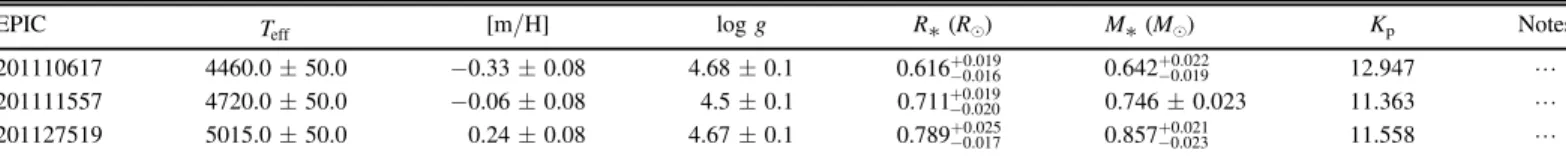
Table 3 Stellar Parameters
EPIC Teff [m/H] log g R* (Re) M* (Me) Kp Notes
201110617 4460.0±50.0 −0.33±0.08 4.68±0.1 0.616+-0.0190.016 0.642-+0.0190.022 12.947 L 201111557 4720.0±50.0 −0.06±0.08 4.5±0.1 0.711-+0.0200.019 0.746±0.023 11.363 L 201127519 5015.0±50.0 0.24±0.08 4.67±0.1 0.789 0.0170.025 -+ 0.857 0.023 0.021 -+ 11.558 L Notes. a
Stellar parameters for this star are derived from a single spectrum with a cross-correlation function peak height<0.9 (but >0.8). We have decided that the resulting stellar parameters are trustworthy for this analysis, but provide a note for the reader’s discretion.
b
SHKvalues have been determined for this star and can be found in Table4. (This table is available in its entirety in machine-readable form.)
4.3. Contrast Curves
We quantified the constraints placed on the presence of additional companions in our high-resolution(speckle and AO) imaging by calculating contrast curves. A contrast curve specifies at a given distance from the target star how bright a companion star would have to be in order to be detected.
After the speckle observations were collected, the data were reduced according to the method described in Furlan et al. (2017), yielding a high-contrast image of a candidate. Then
local minima and maxima were analyzed relative to the star’s peak brightness to determine Δm (average sensitivity) and its uncertainties within bins of radial distance from the target star. The contrast curves used in this research were the 5σupper limit onΔm as a function of radial distance. A more detailed description of the data reduction process can be found in Howell et al. (2011). An example of a contrast curve can be
seen in Figure 6.
As for AO observations, the creation of corresponding contrast curves was performed by injecting fake sources into the images and varying their brightness in order to determine the brightness threshold for the detection algorithm being used. This process is described in greater detail in Crossfield et al. (2016) and Ziegler et al. (2017).
Note that these processes of creating a contrast curve were the same regardless of wavelength. So in the instances that multiple speckle or AO images at different wavelengths were available, multiple contrast curves were created that were all used in the validation process for a given candidate.
5. False-positive Probability(FPP) Analysis 5.1. The Application ofvespa to Planet Candidates Our validation work relied primarily on a method called validation of exoplanet signals using a probabilistic algorithm, orvespa, a public package (Morton2015b) based on the work
of Morton(2012). It operates within a Bayesian framework and
calculates the FPP, the probability that a candidate is an astrophysical false positive rather than a true positive (i.e., a planet).
After photometry, spectroscopy, and any available high-contrast imaging had been collected and reduced for a candidate system, that system underwent our validation procedure using vespa. For each candidate, the following information was supplied:
1. A folded light curve containing the planetary transit and roughly one transit duration of baseline on either side. Identical error bars were assigned to all data points based on the noise parameter determined by our transit-fitting procedure. From this light curve, other planets in the system were removed using the best-fit parameters determined by thefitting procedure.
2. A secondary threshold limit. We calculated this limit by first cutting out all transits from all candidates in a system. Then, for a given candidate, we phase-folded the data to the candidate’s period, binned the baseline flux according to the transit duration of the candidate, calculated the standard deviation between the bin averages, and multiplied by three. Effectively, we assert that a secondary eclipse has not been detected at a 3σ level or higher.
3. A contrast curve. When available, this lowered the FPP by eliminating the possibility of bound or background stars above a certain brightness at a given projected distance, thus reducing the parameter space in which a false-positive scenario could exist. Note thatvespa does
Table 4 Stellar SHKActivity Index
EPIC Date SHK 201437844 2017 Jan 08 0.1666 0.00310.0030 -+ 201437844 2017 Mar 09 0.1698±0.0032 201437844 2017 Mar 09 0.1589±0.0031 201437844 2017 Mar 09 0.1712±0.0031 201437844 2017 Mar 09 0.1651-+0.00290.0030 201437844 2017 Mar 09 0.1624±0.0030 201437844 2017 Mar 09 0.1633 0.00290.0030 -+ 201437844 2017 Mar 09 0.1614±0.0029 201437844 2017 Mar 09 0.1692±0.0029 201437844 2017 Mar 09 0.1622-+0.00290.0030 201437844 2017 Mar 09 0.1635±0.0028 201437844 2017 Mar 09 0.1593-+0.00270.0029 201437844 2017 Mar 09 0.1615-+0.00290.0028 201437844 2017 Mar 09 0.1680-+0.00290.0028 201437844 2017 Mar 09 0.1646±0.0029 201437844 2017 Mar 09 0.1639±0.0028 201437844 2017 Mar 09 0.1651±0.0028 201437844 2017 Mar 09 0.1656±0.0029 201437844 2017 Mar 09 0.1693±0.0029 201437844 2017 Mar 09 0.1641±0.0029 201437844 2017 Mar 09 0.1680±0.0029 205904628 2015 Jul 24 0.1550-+0.00300.0029 205904628 2015 Sep 06 0.1453-+0.00330.0031 211424769 2015 Dec 09 0.3255 0.00390.0040 -+ 211424769 2016 Jan 01 0.3144-+0.00390.0040 211993818 2015 Nov 27 0.4189-+0.00450.0044 211993818 2016 Feb 29 0.3851-+0.00300.0031 211993818 2016 Mar 02 0.3115-+0.00280.0027
Figure 6.Contrast curve developed from a speckle image at 692 nm(6920 Å) for candidate system EPIC 212521166. The contrast curve is plotted asΔm (average sensitivity to a companion in magnitude difference between the primary and secondary) vs. angular separation (in arcseconds). Plus signs and circles are maxima and minima, respectively, of the background sensitivity in the image. The blue squares are the 5σ sensitivity limit within adjacent angular separation annuli. The red line is the contrast curve itself, a splinefit to the sensitivity limit(the blue squares).
11
not require a contrast curve to operate, and in many cases, a candidate host star had no contrast curve data available. However, contrast curves were collected from AO or speckle data and provided to vespa for 186 of our 233 candidate host stars (see Table1).
4. R.A. and Decl. The likelihood of a false-positive scenario is calculated byvespa based on the target star’s location on the celestial sphere. For example, near the Galactic plane, a target star’s FPP will increase significantly due to the crowded field.
5. Teff, log g, and [m/H] (collected from SPC). These constraints help rule out false-positive scenarios that would otherwise be allowed given only stellar magnitude information. Although vespa could operate without these values, we did not apply vespa to any candidate system for which stellar parameters could not be estimated from a TRES spectrum.
6. Stellar magnitudes. The K2 Ecliptic Plane Input Catalog (Huber et al. 2016) was queried to find magnitude
information on each target star in the Kepler J, H, and K bandpasses. The J, H, and K bandpasses originated from the 2MASS catalog (Cutri et al. 2003; Skrutskie et al. 2006). Magnitude uncertainties were not required
or provided for the Kepler bandpass, while uncertainties for the J, H, and K bandpasses were added in quadrature with 0.02 mag of systematic uncertainty to be conservative.
7. Parallaxes. When parallaxes were available from HIP-PARCOS (Perryman et al. 1997) or GAIA (Gaia
Collaboration et al. 2016a, 2016b), they were also
included.
With all this input, vespa makes a representative popula-tion for each false-positive scenario (and the transiting planet scenario). False-positive scenarios considered by vespa include a background(or foreground) eclipsing binary blended with the target star, a hierarchical eclipsing binary system, or a single eclipsing binary system (as well as each of those scenarios with twice the period). Then vespa calculates a prior for each scenario by multiplying the probability that the scenario exists within the photometric aperture, the geometric probability that the scenario leads to an eclipse, and the fraction of instances in which the eclipse is appropriate. Here “appropriate” means that an instance’s eclipse takes place within the photometric aperture, the secondary eclipse (if it exists) is not deep enough to cross the detection threshold, the instance’s primary star has wavelength-dependent magnitudes within 0.1 mag of those provided as input, and the instance’s primary star has Teffand logg that agree with the input values to within 3σ.
Then the likelihood for each scenario is calculated using the folded light curve by fitting against a distribution of transit durations, depths, and ingress/egress slopes calculated from each scenario. When the priors and likelihoods have been determined for each scenario, the last step is simply to combine them for each scenario in order to determine an overall posterior likelihood for every scenario. If the posterior likelihood for the planet scenario is exceedingly higher than all of the other scenarios combined, then the candidate can be classified as a validated planet. In our case, we required the sum of all false-positive scenario probabilities to be <0.001.
The output from vespa includes simulation information from the underlying light-curve fitting process, as well as
figures and text files conveying likelihood information of various false-positive scenarios and the transiting planet scenario. Section 6.1 provides a concrete validation example with characteristic input and output and Table5contains FPP results for all 275 candidates. Additionally, the full vespa input and output for each exoplanet candidate has been archived at10.5281/zenodo.1164791.
As we noted in Section 4.2, for systems where we had collected more than one good TRES spectrum, we phased the RVs to search for or eliminate the possibility of an eclipsing binary scenario.(Small RVs would not rule out hierarchical or background eclipsing binary scenarios since large RVs would be reduced by the third star in the aperture.) In cases where the eclipsing binary scenario could be eliminated, we reduced the probability of the scenario (and the similar scenario analyzed byvespa with twice the period) to zero. We then divided the probability of all the remaining scenarios investigated by vespa by their sum so that the total probability was still one. Systems with multiple planet candidates are more likely to be hosting multiple planets than multiple false-positive signals. In fact, the likelihood of the planet scenario for each individual candidate is consequently boosted relative to false-positive scenarios in multiplanet candidate systems (Latham et al.
2011). To account for this effect, we apply a “multiplicity
boost” to the planet scenario prior in such systems, deflating the FPP by the multiplicity boost factor to account for the nature of these systems. We choose a boost factor of 25 for double-candidate systems and a boost factor of 50 for systems with three or more candidates based on the values used by Lissauer et al. (2012), Vanderburg et al. (2016a), and Sinukoff et al.
(2016). The FPP values reported in Table 2 already have the appropriate multiplicity boost factor applied.
5.2. Criteria for Planet Validation
Following standard practice, we only validated planets for which the following were true, sincevespa assumes we have checked for and ruled out each of them:
1. There is not a composite spectrum.
2. There is not a companion in the aperture. (This was determined from archival imaging.)
3. There is not a companion in AO and/or speckle images. (This was determined from our AO and speckle images as well as from any images for our candidates uploaded to
https://exofop.ipac.caltech.edu/k2/before 2017 August 9.) 4. There is no evidence of a secondary eclipse (at any
arbitrary phase).
5. There is not an ephemeris match(see Section2.4).
If any of the above were false, the FPP was not reported in Table2 and the candidate was not validated regardless of the FPP valuevespa provided.
It is worth noting that six validated planets have recently been shown to be false positives by follow-up observations and analysis(Cabrera et al. 2017; Shporer et al.2017). We briefly
examine whether these instances are a cause for concern in our own results.
In the case of Cabrera et al.(2017), they found that two false
positives exhibited increased transit depths for larger aperture masks (suggesting that a nearby star was responsible for the eclipses), while the third showed a secondary eclipse at phase=0.62 when they used a different data reduction process. The first two false positives would have failed the
Table 5 Detailed FPP Table K2 Name EPIC Secondary Eclipse Threshold (ppm) Aperture Radius
(arcsec) AO/Speckle P(EclipsingBinary)
P(Eclipsing Binary) (x2 Per.) P (Back-ground Eclip-sing Binary) P (Back-ground Eclip-sing Binary) (x2 Per.) P (Hier-archical Eclipsing Binary) P(Hier-archical Eclipsing Binary) (x2 Per.) RV Mass Limit VESPA FPP Multiplicity
Boost Adopted FPP Disposition
K2-156 b 201110617.01 28 14.7 Y 0.00e+00 0.00e+00 <1e-04 <1e-04 <1e-04 <1e-04 Y 2.18e-08 L <1e-04 Planet
201111557.01 47 14.4 Y <1e-04 1.16e-03 <1e-04 <1e-04 <1e-04 <1e-04 N 1.22e-03 L 1.22e-03 Candidate
201127519.01 813 17.9 Y L L L L L L Y L L L Candidate
(This table is available in its entirety in machine-readable form.)
13 The Astronomical Journal, 155:136 (25pp ), 2018 March Mayo et al.
variable-sized mask test we apply via our diagnostic plots, while the secondary eclipse from the third false positive would have been caught through a combination of our data reduction process and the model-shift uniqueness test we apply (Coughlin et al.2016).
As for Shporer et al.(2017), the vespa fit to the available
photometry for each false positive was very poor and all three of the false positives were reported to be very large“planets.” We addressed these concerns in two ways. First, we decided to only use 2MASS photometry in order to avoid systematic errors between photometric bands. Second, we chose not to validate any planet candidates larger than 8 R⊕, since a candidate of that size or larger could actually be a small M dwarf. The only exception to this rule is if there are RV measurements that can rule out the eclipsing binary scenario, in which case we do report the FPP (and validate for FPP<0.001), regardless of planet size.
6. Results
The results section is divided into two parts. In thefirst part, the process of validation is described in detail for a single planet candidate, in order to explain precisely how the photometry and follow-up observations are used. In the second part, our validation process is more widely applied to every selected candidate, and the results for each candidate are reported.
6.1. Validating a Single Planet: EPIC 212521166.01 In order to understand the process that was applied to each of our candidates, it is instructive to look at validation for a single, concrete example. Here, we describe in detail the validation process for a typical planet candidate system, EPIC 212521166 (K2-110). We chose this system because (1) it was detected in our pipeline, and (2) Osborn et al. (2017) have already
confirmed and characterized the planet, which allows us to compare some of the system parameters we calculated with their results.
EPIC 212521166 was observed by K2 during Campaign 6. After we produced a light curve from calibrated K2 pixel data and removed systematics (as described in Section 2.2), we
searched for transits in our processed light curve (as described in Section 2.3). Our transit search pipeline detected a single
TCE with a high S/N, a period of 13.87 days and a depth of about 0.1%. The signal passed triage (see Section 2.3) and
moved on to vetting(see Section 2.4). We confirmed that the
signal was transit-like, and observed no significant secondary eclipse, phase variations, differences in depth between odd and even transits, aperture-size dependent transit depths, or other indications of a false-positive or instrumental false alarm(see Figures 2–4). As a result, we promoted the EPIC 212521166
TCE to a planet candidate.
Upon its identification as a planet candidate, we observed EPIC 212521166 with the TRES spectrograph on the Mt. Hopkins 1.5 m Tillinghast reflector and with the DSSI speckle-imaging camera on the 3.5 m WIYN telescope at Kitt Peak National Observatory. Using the orbital and transit parameters determined with our transit model, the stellar parameters derived from SPC, a folded light curve of the planetary transit, and two contrast curves in r band and z band collected via high-contrast speckle imaging from DSSI on the WIYN telescope (see Figure6), vespa was employed to determine the FPP for
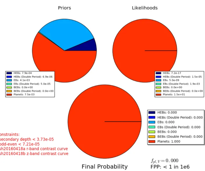
EPIC 212521166.01. The FPP was found to be 8.44×10⁻⁷, which was well below the cutoff threshold, so the planet candidate was classified as validated. The key output figure of vespa can be seen in Figure7.
Like us, Osborn et al.(2017) found EPIC 212521166 to be a
metal-poor K-dwarf star hosting planet candidate with P=13.9 day and Rp=2.6 R⊕. A comparison of planetary and system parameters can be see in Table6. Our analyses and theirs are in good agreement for all parameters. Additionally, Osborn et al.(2017) took the further step of obtaining precise
RV observations to confirm the existence of EPIC 212521166.01, so we can be confident that in this case, the assessment byvespa of a low FPP was well justified.
6.2. Full Validation Results
The process of validation described for EPIC 212521166.01 in the previous section was similarly applied to the remaining candidates suitable for validation. We identified 275 candidates in 233 systems that had at least one usable TRES spectrum, and the FPP was calculated for each of these candidates (see Table2).
Occasionally,vespa failed to return an FPP; in such cases, the lowest data point in the light curve was removed(to aid the initialization process for thevespa trapezoidal transit fit), and vespa was rerun. This approach worked in most cases, but if it failed, the lowest two data points were removed andvespa was rerun. If that was also unsuccessful, then the FPP was not reported.(Most of the time, vespa only failed after these steps because of a Roche lobe overflow error.) 149 candidates in 111 systems had an FPP<0.001 and were thus promoted to validated planet status.
To date, the largest single release of K2 validation results has been Crossfield et al. (2016), with 197 candidates and 104
validated planets in C0–C4. In comparison, 108 of our candidates are from C0–C4, 69 of which are validated. The two samples share 53 candidates in common, 37 of which are validated and 9 of which remain candidates in both analyses. (Additionally, 2 candidates in common are only validated in this work, while 5 are only validated in Crossfield et al.2016.) This leaves 55 candidates in our C0–C4 sample (30 of which are validated) that were undetected by Crossfield et al. (2016),
as well as 146 candidates (62 of which are validated) in the Crossfield et al. (2016) sample that are undetected in our own
C0–C4 sample. Only ∼21% of the total candidates were detected by both analyses, and only ∼26% of the total validated planets were validated by both analyses.
The sample overlap may seem surprisingly small, but it makes more sense when the candidate selection and validation processes are examined. For example, Crossfield et al. (2016)
only considered candidates with 1 day<P<37 day (19% of our C0–C4 sample was outside that range), and we only considered candidates with Kp<13 (48% of their sample was outside that range). If we only consider C0–C4 candidates within those ranges (137 total), both teams find over half of each other’s samples, and the overlap between samples rises to 39% (53 candidates). Similarly, for validated planets within these ranges(77 total), both teams find more than two-thirds of each other’s samples, and the overlap between samples rises to 57%(44 validated planets).
There are many further examples of differences that created discrepancies between the two samples. We required that each planet candidate had at least one usable TRES spectrum (see
Sections 3.1and 4.2), even though in early campaigns, TRES
spectra were not collected for all bright candidates. This led to the exclusion of many otherwise promising candidates that are included in Crossfield et al. (2016). Further discrepancies could
have arisen from the temperature and planet radius cuts applied to our validated planet sample, the elimination of objects with companions closer than 4″in the Crossfield et al. (2016)
candidate sample, and a difference in significance thresholds for TCEs(we used 9σ, while they used 12σ).
Table 7 compares the candidate dispositions found in this work with their previous dispositions (according to the NASA Exoplanet Archive32 and the Mikulski Archive for Space Telescopes33; both accessed 2018 February 14). We should note that 15 of our candidates were not validated in this work even though they have been previously validated elsewhere.
However, all of these candidates were either restricted from being validated by our conservative criteria for validation (see Section5.2), had an FPP value close to our validation cutoff of
FPP=0.001, or were validated using different or additional observations as input to vespa. We also note that our work classifies two targets that have previously been labeled as false positives: EPIC 202900527.01 (K2-51 b) and EPIC 2108940 22.01 (K2-111 b). Shporer et al. (2017) clearly showed EPIC
202900527.01 to be a stellar binary. We do not claim otherwise by labeling it a candidate (since we label all targets with FPP>0.001 as candidates). On the other hand, Crossfield et al. (2016) previously identified EPIC 210894022.01 as a false
positive, but a subsequent, improved vespa run showed the target to in fact be a planet (I. Crossfield 2017, private communication). Therefore we do claim this target to be validated. Another case worth mentioning is the multiplanet system EPIC 228725972, which hosts one validated planet and one candidate ruled out by a companion in the aperture and in a
Figure 7.False-positive probability analysis of EPIC 212521166.01. HEB, EB, and BEB refer to a hierarchical eclipsing binary, eclipsing binary, and background eclipsing binary scenario, respectively. Combining the prior likelihood of a false-positive scenario(given sky position, contrast curve data, and wavelength-dependent magnitudes), as well as the likelihood of the transit photometry under various scenarios, the posterior distribution highly favors the planet scenario, with FPP=8.44×10⁻⁷.(Note: the true FPP value is always reported in a supplementary file, but for FPP<1 in 1e6, the figure produced by vespa simply reports the FPP as<1 in 1e6.)
32https://exoplanetarchive.ipac.caltech.edu/ 33
https://archive.stsci.edu/k2/published_planets/search.php
15