HAL Id: hal-00468602
https://hal.archives-ouvertes.fr/hal-00468602
Submitted on 31 Mar 2010
HAL is a multi-disciplinary open access
archive for the deposit and dissemination of
sci-entific research documents, whether they are
pub-lished or not. The documents may come from
teaching and research institutions in France or
abroad, or from public or private research centers.
L’archive ouverte pluridisciplinaire HAL, est
destinée au dépôt et à la diffusion de documents
scientifiques de niveau recherche, publiés ou non,
émanant des établissements d’enseignement et de
recherche français ou étrangers, des laboratoires
publics ou privés.
Optimal Reconstruction Might be Hard
Dominique Attali, André Lieutier
To cite this version:
Dominique Attali, André Lieutier. Optimal Reconstruction Might be Hard. SoCG 2010 - 26th Annual
Symposium on Computational Geometry, Jun 2010, Snowbird, Utah, United States. pp.334-343,
�10.1145/1810959.1811014�. �hal-00468602�
Optimal Reconstruction Might be Hard
∗[Extended Abstract]
Dominique Attali
Gipsa-lab, Grenoble, France
[email protected]
André Lieutier
Aix-en-Provence, France
[email protected]
ABSTRACT
Sampling conditions for recovering the homology of a set using topological persistence are much weaker than sam-pling conditions required by any known polynomial time algorithm for producing a topologically correct reconstruc-tion. Under the former sampling conditions which we call weak sampling conditions, we give an algorithm that out-puts a topologically correct reconstruction. Unfortunately, even though the algorithm terminates, its time complexity is unbounded. Motivated by the question of knowing if a polynomial time algorithm for reconstruction exists under the weak sampling conditions, we identify at the heart of our algorithm a test which requires answering the follow-ing question: given two 2-dimensional simplicial complexes L⊂ K, does there exist a simplicial complex containing L and contained in K which realizes the persistent homology of L into K? We call this problem the homological simpli-fication of the pair (K, L) and prove that this problem is NP-complete, using a reduction from 3SAT.
Categories and Subject Descriptors
F.2.2 [Analysis of Algorithms and Problem Complex-ity]: Nonnumerical Algorithms and Problems—Geometrical problems and computations, Computations on discrete struc-tures; I.3.5 [Computer Graphics]: Computational Geom-etry and Object Modeling
General Terms
Algorithms, Theory
Keywords
Shape reconstruction, topological persistence, sampling con-ditions, homological simplification, NP-completeness, 3SAT ∗This work is partially supported by ANR Project GIGA ANR-09-BLAN-0331-01.
Permission to make digital or hard copies of all or part of this work for personal or classroom use is granted without fee provided that copies are not made or distributed for profit or commercial advantage and that copies bear this notice and the full citation on the first page. To copy otherwise, to republish, to post on servers or to redistribute to lists, requires prior specific permission and/or a fee.
SCG’10,June 13–16, 2010, Snowbird, Utah, USA. Copyright 2010 ACM 978-1-4503-0016-2/10/06 ...$10.00.
1.
INTRODUCTION
Previous works.
In the last decade, several authors have proposed algo-rithms for reconstructing shapes with topological guaran-tees. First results considered compact smooth surfaces em-bedded in the Euclidean three-dimensional space and as-sumed surfaces to be known through noise-free samples [5, 1, 3, 9, 22, 4]. Since then, an effort has been made to gen-eralize such results to wider classes of shapes and sampling conditions [24, 21, 32, 15, 10, 25].
An important extension allows samples to be noisy: each point of the sample is required to lie within some distance of the sampled shape (the sample is accurate) and each point of the sampled shape must lie within some distance of a sample point (the sample is dense). When both distances are bounded by the same value ε, the sampling condition can be expressed by saying that the Hausdorff distance between the shape and the sample is upper bounded by ε.
In 2006, several algorithms for reconstructing non-smooth objects with topological guarantees have been designed. In [33, 11], Boissonnat and Oudot considered Lipschitz mani-folds while Chazal, Cohen-Steiner and Lieutier in [12] con-sidered a large class of non-smooth compact sets called sets with positive µ-reach. In particular, the latter gave a poly-nomial time algorithm that is able to output what we will call in the paper a faithful reconstruction (see Definition 1). In 2002, a fruitful point of view in computational topol-ogy, called topological persistence, has been introduced [26]. Within this context, the theorem on the stability of persis-tence diagrams [18] allows to infer the homology of shapes known through a sample. The sampling condition is sig-nificantly milder than the one required by the previously mentioned algorithm for computing a faithful reconstruc-tion. We refer to this mild sampling condition sufficient for recovering homology as the weak sampling condition. This condition is tight.
Optimal reconstruction.
We call any algorithm that would be able to produce a faithful reconstruction under the weak sampling condition an optimal reconstruction algorithm. We explain in Sec-tion 2.3 that, even though no realistic version of an opti-mal reconstruction algorithm is known today, the weak sam-pling condition ensures that the sample contains in principle enough information on the sampled shape to produce with-out ambiguity a faithful reconstruction of it. Starting from this observation, we give in Section 2.4 a “naive” algorithm
which, at the expense of not being efficient, produces a faith-ful reconstruction under the weak sampling condition.
The main question we pursue is: can we do better? More precisely, does there exist a polynomial time optimal recon-struction algorithm? Such an algorithm would have ap-plications in several fields such as shape reconstruction or machine learning. While [6] gives a partially positive an-swer for subsets of R2, the question remains open for higher dimensions. Indeed, this problem is closely related to the persistence-sensitive simplification of real-valued functions, whose goal is to filter out topological noise in sub-level sets. Indeed, reconstruction can be thought of as the simplifi-cation of distance functions to the samples. For functions defined on triangulated 2-manifolds, polynomial algorithms have been devised [27, 6, 30]. Still, persistence-sensitive sim-plification of functions in higher dimension remains elusive.
Homological simplification.
In Section 3, we focus on the test at the heart of our naive algorithm. This test requires to answer the following question: given two 2-dimensional simplicial complexes L⊂ K, does there exist a simplicial complex X containing L and contained in K such that the maps induced by the inclusions L ֒→ X and X ֒→ K on all modulo 2 homology groups are respectively surjective and injective. We call this problem the homological simplification of the pair (K, L) and prove that it is NP-complete.
Although this result is negative, we believe that it casts new light on the problem of finding a faithful reconstruc-tion under weak sampling condireconstruc-tions and opens further re-search tracks as mentioned in Section 4. In particular, it suggests that, in order to design efficient reconstruction al-gorithms under weak sampling conditions, one has to make additional hypotheses. For instance, one can assume shapes are embedded in R3 and/or require some specific properties on embedded simplicial complexes.
2.
THE QUEST FOR AN OPTIMAL
RECON-STRUCTION ALGORITHM
Section 2.1 presents the necessary background. Section 2.2 contains our definition of a (homological) faithful re-construction. We then define weak sampling condition and optimal reconstruction algorithms in Section 2.3. Finally, Section 2.4 presents a naive algorithm that outputs a homo-logical faithful reconstruction under a condition approaching the weak sampling condition.
2.1
Background
The goal of this section is to recall three closely related concepts useful for the expression of sampling conditions in shape reconstruction. Given a shapeA, we define the reach r1(A), the µ-reach rµ(A) for any µ ∈ (0, 1] and the weak feature size wfs(A). As we shall see, these quantities are re-lated by the following inequality: r1(A) ≤ rµ(A) ≤ wfs(A). All three concepts can be derived from the critical function of the shape. This leads us to introduce the critical function, which requires first to define the norm of the gradient to the distance function.
The distance function to a compact set plays a central role in several recent works related to topologically guaranteed reconstruction [29, 23, 12]. For a compact setA ⊂ RN, the distance function dA: RN → R+ maps every point q∈ RN
to
dA(q) = min
a∈Aka − qk.
Although not differentiable, dAadmits several extended no-tions of gradient [16, 29]. For our purpose, we will intro-duce a real valued function ΨA : RN \ A → [0, 1] which corresponds to the norm of the gradient defined in [29]. Let
d
dt+(·)|t=0 denote the right derivative with respect to the variable t at t = 0. For q∈ RN
\ A and v ∈ SN −1, one can check [29] that the quantity d
dt+dA(q +tv)|t=0is well-defined and belongs to [−1, 1]. We define ΨAas:
ΨA(q) = max ( 0, sup v∈SN −1 d dt+dA(q + tv)|t=0 ) . Roughly speaking, ΨA(q) quantifies at which maximal speed the distance function to A can increase in a neighborhood of q. We are now ready to recall the definition of the critical function χA introduced in [12]. The critical function maps every positive real number ρ > 0 to the infimum of ΨAover the set of points at distance ρ fromA:
χA(ρ) = inf dA(q)=ρ
ΨA(q).
The critical function is lower semi-continuous [12] and allows to define two quantities, the µ-reach and the weak feature size ofA denoted respectively rµ(A) and wfs(A):
rµ(A) = inf {ρ > 0, χA(ρ) < µ} , wfs(A) = inf {ρ > 0, χA(ρ) = 0} .
The reach of A is equal to r1(A). From the definition, it is clear that r1(A) ≤ rµ(A) ≤ wfs(A) for any µ ∈ (0, 1]. Figure 1 shows the critical function χA for a simple shape A in the Euclidean plane, which consists of the points at distance R from a full rectangle of width ℓ and length L.
R 1 1 √ 2 R + ℓ 2 χA(ρ) ρ A ℓ + 2 R L + 2R R
Figure 1: Left: the shapeA is the outer closed thick curve and its medial axis consists of the five thin inner segments. Right: critical function χA. We have rµ(A) = R for µ >√1 2 and rµ(A) = R + l 2 = wfs(A) for µ≤√1 2.
To shed light on these notions, it is useful to make some connections with the medial axis. The medial axis of A is the set of points q /∈ A which have at least two closest points in A. Alternatively, it is the locus of points q for which ΨA(q) < 1. Any point q for which ΨA(q) = 0 is called a critical point of the distance function and lies on the medial axis. The reach is the minimum of distances between points inA and in its medial axis. The weak feature size is the minimum of distances between points inA and critical points.
For instance, the function ΨAof the shapeA depicted in Figure 1 evaluates to 0 on the horizontal line of the medial axis which constitutes the only critical points in this case, evaluates to √1
2 on the other points of the medial axis and evaluates to 0 on all points of the plane that neither belong toA nor to its medial axis.
For completeness, we also recall the related notion of lo-cal feature size, introduced by Amenta [2] for reconstructing smooth shapes. The local feature size is a real-valued func-tion which maps every point of A to its distance to the medial axis. Notice that the local feature size and its infi-mum, the reach, vanish on non-smooth objects as soon as they contain a sharp concave corner or edge. For this reason, we will focus in Section 2.3 on sampling conditions based on the weak feature size and µ-reaches which apply to a large class of non-smooth shapes.
Given η > 0, the η-offset of A is the set of points at distance η or less fromA, Aη = d−1
A ([0, η]). As in Morse theory, topological changes in offsets occur only at critical values. More precisely, as stated in [28, 14]:
Lemma 1 (Topological Stability of Offsets). If 0 < x < y < wfs(A), then the inclusion map Ax֒→ Ayis a homotopy equivalence.
2.2
Faithful reconstructions
Let us now give our definitions of a faithful reconstruc-tion and a faithful homological reconstrucreconstruc-tion. For the sec-ond definition, we will consider a fixed field F and take co-efficients in F for homology [31, Chapter 1]. Hence, the property of being a faithful homological reconstruction will depend on the choice of F .
Definition 1. We say that a subsetR ⊂ RNis a faithful reconstruction of the compact setA ⊂ RN if there exist real numbers x, y such that 0 < x < y < wfs(A) and the following two properties hold:
• Ax⊂ R ⊂ Ay
• the inclusion maps Ax֒
→ R and R ֒→ Ay are homo-topy equivalences.
We say thatR is a faithful homological reconstruction when the last condition is relaxed by:
• the inclusion maps Ax ֒
→ R and R ֒→ Ay induces isomorphisms on all homology groups.
A faithful reconstruction is always a faithful homological re-construction. As expected, the converse is not true: a punc-tured Poincar´e sphere nested between a point and a ball is an example where inclusions are not homotopy equivalences but yet induce isomorphisms on homology groups [17]. In-terestingly, this example does not embed in R3.
Note that in the above definition, if one of the two inclu-sion mapsAx֒
→ R or R ֒→ Ayis a homotopy equivalence, so is the other one. Indeed, by Lemma 1, Ax ֒
→ Ay is a homotopy equivalence and we can conclude by applying Lemma 2 below. A similar statement can be made for the second part of the definition.
Lemma 2. Consider three nested spacesA ⊂ B ⊂ C. If two of the three inclusions i : A ֒→ B, j : B ֒→ C and k = j◦ i : A ֒→ C are homotopy equivalences, then the third one is also a homotopy equivalence.
Proof. If i and j are homotopy equivalences with homo-topy inverses i′ and j′ respectively, then i′◦ j′ is clearly a homotopy inverse of k = j◦ i.
If j and k are homotopy equivalences with homotopy in-verses j′and k′respectively, then using k = j◦ i we get that j′◦ k = j′◦ j ◦ i ≃ i and k′◦ j is a homotopy inverse of i≃ j′◦ k.
Similarly, if i and k are homotopy equivalences with ho-motopy inverses i′ and k′ respectively, then using k = j◦ i we get that k◦ i′ = j◦ i ◦ i′ ≃ j and i ◦ k′ is a homotopic inverse of j≃ k ◦ i′.
2.3
Sampling conditions
In this section, we compare inputs, preconditions and out-puts of two algorithms that infer information on a shapeA known through a finite sample S. Specifically, the first al-gorithm recovers Betti numbers of A and the second one constructs a faithful approximation of A. Each algorithm relies on a key theorem that states sampling conditions en-suring correctness. Both algorithms are polynomial in the size of the sample. We then define an optimal reconstruction algorithm as one that would produce the output of the sec-ond algorithm with the input and precsec-ondition of the first algorithm.
We recall that the Hausdorff distance between two com-pact setsA and A′ of RN is defined by:
dH(A, A′) =kdA′− dAk
∞= sup q∈RN|dA
′(q)− dA(q)|.
Computing Betti numbers.
A powerful tool for inferring Betti numbers from geomet-ric approximations is topological persistence [26]. Theorem 3 below is a corollary of the Persistence Stability Theorem [18] and can also be derived by flow based arguments [14]. Before stating it, we need the following definition.
Definition 2. LetA ⊂ RN be a compact set and let 0 ≤ x≤ y. The p-th (x, y)-persistent Betti number of A is the rank of the homomorphism induced by inclusionAx֒
→ Ay: βpx,y(A) = rank (Hp(Ax) ֒→ Hp(Ay))
It is worth noting that the (x, y)-persistent Betti numbers are finite whenever x < y [20].
Theorem 3 (Homology Inference [18, 14]). LetA andS be two compact subsets of RNand suppose there exists a real number α > 0 such that
dH(S, A) < α < 1 4wfs(A) Then, βp(A) = βα,3α
p (S).
The above theorem leads immediately to a polynomial time algorithm for inferring Betti numbers of a shape A when the sample S of A is finite. Indeed, writing Kα(S) for the α-complex ofS, the persistent Betti numbers can be expressed as
βpα,3α(S) = rank (Hp(Kα(S)) ֒→ Hp(K3α(S))) . In particular, they can be computed in time cubic the size of K3α(S). Since for a fixed dimension, the size of α-complexes is polynomial in the number of vertices, it follows that βp(A) can also be computed in polynomial time the size of the sample.
Table 1: Input, precondition and output of two polynomial time algorithms derived from Theorem 3 and Theorem 4. The notation “∃A” stands for “there exists a compact set A ⊂ RN”.
S designates a finite set of RN. α and µ designate two real numbers with α > 0 and µ∈ (0, 1].
Input Precondition Output
S, α ∃A, dH(S, A) < α < 14wfs(A) Betti numbers ofA S, α, µ ∃A, dH(S, A) < α < µ
2
5µ2+12rµ(A) a faithful reconstruction ofA
Computing a faithful reconstruction.
For a shape A with a positive µ-reach, authors in [12] describe a simple procedure for computing a faithful recon-struction ofA, given as input a sample S of A. The proce-dure consists merely of outputting an r-offset of the sample, for a suitable value of the offset parameter r (see Theorem 4 below for the precise value of r). In practice, this compu-tation can be replaced by the compucompu-tation of Kr(S), which shares the same homotopy type. Both computations can be done in polynomial time if the sample is finite. The sam-pling condition required by the procedure is that the Haus-dorff distance between the sampleS and the sampled shape A is less than a fraction the µ-reach of A. More precisely:
Theorem 4 (Reconstruction Theorem [12]). LetA andS be two compact subsets of RN and suppose there exists two real numbers α > 0 and µ∈ (0, 1] such that
dH(S, A) < α < µ 2
5µ2+ 12rµ(A) Then,S4αµ2 is a faithful reconstruction ofA.
Comparing sampling conditions.
Table 1 summarizes inputs, preconditions and outputs of the two polynomial time algorithms described above and in-spired by Theorems 3 and 4. Note that the precondition required by the first algorithm which we call the weak pre-condition is equivalent to saying that the following set is non-empty: W (S, α) = X | dH(S, X ) < α < 1 4wfs(X ) ff 6= ∅, (1) whereX ranges over all compact sets of RN. By Theorem 3, all shapes in W (S, α) share the same Betti numbers and the first algorithm returns the Betti numbers of any A ∈ W (S, α). Since rµ(A) is by definition upper bounded by wfs(A), the first precondition is significantly weaker than the second precondition, especially when µ is small. We now claim that, in some sense, the input of the first algorithm together with its weak precondition determines completely the output of the second. Indeed, let us recall from [14] the following theorem:
Theorem 5 ([14]). Let A and X be two compact sub-sets of RN and α > 0 a real number such that
dH(A, X ) < 2α < 1
2min{wfs(A), wfs(X )} Then,X2αis a faithful reconstruction of
A.
SupposeA and X both belong to W (S, α). Applying a tri-angular inequality, we get thatA, X and α fulfill conditions of Theorem 5 and therefore,X2αis a faithful reconstruction of A. Hence, any 2α-offset of a shape X ∈ W (S, α) is a faithful reconstruction of any shapeA ∈ W (S, α). In other words, all shapes in W (S, α) share a common set of faithful reconstructions which contains 2α-offsets of W (S, α). For this reason, we say that, under the weak precondition, in-puts S and α carry in principle enough information about the unknown shape A to determine without ambiguity a faithful reconstruction of it.
Optimal reconstruction algorithms.
The weak precondition is tight, by which we mean that for any η > 0, the set Wη(S, α) = {X compact set of RN
| dH(S, X ) < α <1
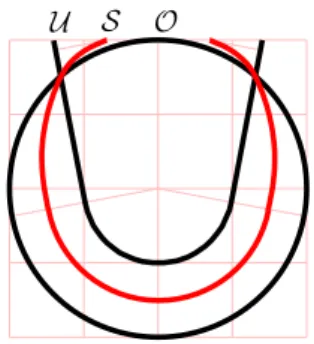
4wfs(X ) + η} may contain objects that do not have the same homology. To construct such an example, consider the two shapes O and U described in [14] and the sample S pictured on Figure 2. By construction, we have wfs(O) = 2, wfs(U) = +∞ and dH(S,O) = dH(S,U) =
1+η
2 . Hence, both O and U belong to Wη(S, 1 2 +
3η 4) but β1(O) 6= β1(U). Therefore, the weak precondition is the weakest amongst the preconditions expressed in terms of Hausdorff distance and critical functions that allows to re-trieve a faithful reconstruction without ambiguity.
U S O
Figure 2: The angle between the two bars in shape U is adjusted such that dH(S, O) = dH(S, U) = 1+η2 .
Because of that, we call any algorithm that would be able to output a faithful reconstruction under the weak pre-condition and associated inputs an optimal reconstruction algorithm. In Section 2.4, we describe a naive algorithm that outputs a faithful homological reconstruction under the weak precondition. We call it “naive” since it has an un-bounded time complexity. The main question motivating our work is whether there exists a polynomial time opti-mal reconstruction algorithm. Section 3 suggests a negative answer if no additional condition is assumed.
2.4
Naive algorithms for reconstruction
Given as input a pair (S, α) satisfying the weak precondi-tion, the previous section suggests the following strategy for computing a faithful reconstruction: enumerate all compact sets in RN and return the 2α-offset of the first compact set X that belongs to W (S, α). Of course, this procedure is un-realistic and the goal of this section is to present an effective version of it. Specifically, given as input a sampleS and two real numbers α and η satisfying the precondition:
∃A, dH(S, A) < α <14(wfs(A) − η), (2) we describe an algorithm that computes a faithful homolog-ical reconstruction ofA and whose pseudocode is given in Table 2. The idea is to replace the enumeration on compact sets by an enumeration on cubical sets and refine the size of the cubes until we find a solution. We also simplify the prob-lem, replacing the search for a faithful reconstruction by the search of a faithful homological simplification. We proceed in two steps. First, we give an algorithm for shapes with a positive µ-reach (NAIVE_1) and then, derive an algorithm for shapes with a lower bounded weak feature size (NAIVE_2).
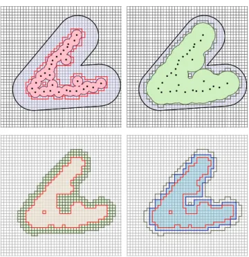
Figure 3: Left: the cubical set (in pink) is nested between two offsets (in light purple) of the V-shaped black curve and is a faithful reconstruction of it. Right: offsetsSl and
Sk of the sample.
We start with some definitions. An ε-voxel is a closed cube with edge length ε and whose vertices belong to the lattice εZN. We call any finite union of ε-voxels an ε-cubical set. Assuming a shapeA has a positive µ-reach, next lemma states the existence of a cubical set which is a faithful re-construction ofA. This is a key ingredient in establishing the correctness of the naive algorithms.
Lemma 6. There exists a positive constant cN depending only upon the ambient dimension N such that the following property holds: for all real numbers x, y and µ∈ (0, 1] and all compact setsA ⊂ RN satisfying rµ(
A) > y > x > 0, there exists a (cNµ(y− x))-cubical set X such that Ax
⊂ X ⊂ Ay and the inclusion mapsAx֒
→ X and X ֒→ Ayare homotopy equivalences. In particular, the cubical set X is a faithful reconstruction ofA (see Figure 3, left).
The proof is in the appendix and relies on a result in [8].
First naive reconstruction algorithm.
Under precondition (2), the algorithmNAIVE_1outputs
ei-ther the empty set or a faithful homological reconstruction
Figure 4: Illustration of algorithm NAIVE_1. Top:
boundaries ofL = Vε(Sl) and
K = Vε(Sk) are depicted in red and dark green. Bottom: the cubical set X in blue is nested between L and K and is a faithful homological reconstruction of A.
ofA. Its pseudocode is given in Table 2, left. The algorithm proceeds as follows. It chooses a voxel size ε, two offset pa-rameters l and k and derives from the sampleS two ε-cubical setsL = Vε(Sl) and
K = Vε(Sk), obtained by collecting all ε-voxels intersecting respectivelySl and
Sk (see Figures 3 and 4). For all cubical setsX containing L and contained in K, the algorithm then considers three nested simplicial complexes L⊂ X ⊂ K triangulating the three cubical sets L ⊂ X ⊂ K in a way that is consistent with the grid. It then returnsX if the simplicial complex X is a homological simplification of the pair (K, L) (see definition below). If no homological simplification X is found between L and K, the algorithm returns the empty set.
Definition 3 (Homological simplification). Let L⊂ K be two simplicial complexes. The simplicial complex X is said to be a homological simplification of the pair (K, L) if L ⊂ X ⊂ K and the maps j∗ : Hp(L) → Hp(X) and i∗: Hp(X)→ Hp(K) induced by inclusions are respectively surjective and injective for all integers p≥ 0 (see Figure 5).
Hp(L) j∗
>Hp(X) i∗
>Hp(K) Figure 5: Notations for Definition 3 and the proof of Lemma 7.
The correctness of the algorithm relies on several lemmas stated in the appendix. Under precondition (2), if X is a homological simplification of the pair (K, L), then Lemma 12 implies thatX = |X| is a faithful homological reconstruction
Table 2: Naive reconstruction algorithms. |X| denotes the underlying space of the simplicial complex X. sc(X ) denotes a triangulation of the cubical set X compatible with inclusion.
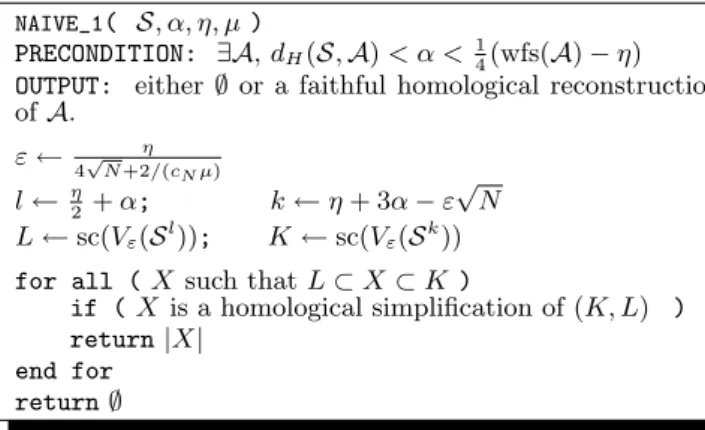
NAIVE_1( S, α, η, µ )
PRECONDITION: ∃A, dH(S, A) < α <14(wfs(A) − η) OUTPUT: either∅ or a faithful homological reconstruction ofA. ε← 4√ η N +2/(cNµ) l← η 2 + α; k← η + 3α − ε √ N L← sc(Vε(Sl)); K ← sc(Vε(Sk)) for all (X such that L⊂ X ⊂ K )
if (X is a homological simplification of (K, L) ) return|X| end for return∅ NAIVE_2(S, α, η ) PRECONDITION: ∃A, dH(S, A) < α <14(wfs(A) − η) OUTPUT:a faithful homological reconstruction ofA µ← 1 α′← α +η 8 η′ ← η 4 while ( TRUE ) X ←NAIVE_1(S, α′, η′, µ) if (X != ∅ ) return X µ←µ2 end while
ofA. Furthermore, under the stronger precondition (3): ∃A, dH(S, A) < α <1
4(rµ(A) − η) , (3) Lemma 11 guarantees that the algorithm always returns a faithful homological simplification (and not∅). Let us bound the time complexity of a more efficient version of the algo-rithm in which voxels are not decomposed into simplices. Let D be the diameter ofS and set D′= D + 2(ν + 3α). It is not difficult to check that this simpler algorithm has time complexity O“2|K||K|3”= O „ 2 “ D′ ε ”N“ D′ ε ”3N« . Indeed, the size of K is O((D′/ε)N). Checking if X is a homological simplification of (K, L) takes cubic time the size of K and the number of cubical setsX between L and K is O(2|K|).
Second naive reconstruction algorithm.
Under precondition (2), the algorithm NAIVE_2outputs a
faithful homological reconstruction ofA after a finite num-ber of iterations. Its pseudocode is given in Table 2, right. Starting with µ = 1, it callsNAIVE_1with decreasing values
of µ untilNAIVE_1returns a faithful homological reconstruc-tion. The algorithm terminates thanks to the lower semi-continuity of the critical function χA. Indeed, χA attains its minimum µ′ > 0 over the interval [η8, 4α + 7η8]. Setting A′ = Aη8, α′ = α + η
8 and η′ = η
4, we have rµ′(A′) > 4α + 3η4 = 4α′+ η′ (see Figure 6 for an explanation) and therefore precondition (3) is satisfied for A = A′, α = α′, µ = µ′ and η = η′. Note that even though the algorithm terminates, its time complexity is unbounded.
χAr(ρ) r 0 µ′ ρ χA(ρ) R
Figure 6: Performing an r-offset translates into translating the critical function to the left by r [12]. Thus, χA(ρ)≥ µ′ on [r, R] implies rµ′(Ar) > R− r.
3.
HOMOLOGICAL SIMPLIFICATION IS
NP-COMPLETE
In this section, we focus on the problem of computing a homological simplification and prove that this problem is NP-complete. We denote the p-th homology group of K by Hp(K) and work with coefficients in the field Z2 of integers modulo 2. A simplicial pair (K, L) consists of a (finite) simplicial complex K and a subcomplex L⊂ K. When clear from the context, we will simply speak of the pair (K, L) and omit “simplicial”. We say that the pair (K, L) is p-dimensional if the simplicial complex K has dimension p.
Definition 4. The homological simplification problem takes as input a simplicial pair (K, L) and asks whether there exists a simplicial complex X which is a homological simpli-fication of the pair (K, L).
The size of the problem is the number of simplices in K. A useful observation is that since we are working with co-efficients in Z2 and homology groups are finite-dimensional vector spaces, X is a homological simplification of the pair (K, L) if and only if X realizes the persistent homology of L into K. Formally, we have:
Lemma 7. Consider a sequence of simplicial complexes L⊂ X ⊂ K. The simplicial complex X is a homological sim-plification of the pair (K, L) if and only if Hp(X) is isomor-phic to the image of the homomorphism Hp(L) → Hp(K) induced by the inclusion L⊂ K, for all integers p ≥ 0.
Proof. See Figure 5. If X is a homological simplifi-cation of the pair (K, L), then the injectivity of the map i∗: Hp(X)→ Hp(K) induced by the inclusion X⊂ K im-plies that Hp(X) is isomorphic to i∗(Hp(X)) and the surjec-tivity of the map j∗: Hp(L)→ Hp(X) induced by inclusion L ⊂ X implies that Hp(X) = j∗(Hp(L)). It follows that Hp(X) is isomorphic to i∗◦ j∗(Hp(L)) for all p.
Conversely, suppose Hp(X) is isomorphic to i∗◦j∗(Hp(L)). Then, j∗ is surjective because dim j∗(Hp(L)) ≥ dim i∗◦ j∗(Hp(L)) = dim Hp(X). Furthermore, i∗ is injective be-cause the surjectivity of j∗implies i∗(Hp(X)) = i∗◦j∗(Hp(L)) which is isomorphic to Hp(X).
Theorem 8. The homological simplification problem of 2-dimensional simplicial pairs is NP-complete.
Proof. To check that a candidate X is a homological simplification of the p-dimensional pair (K, L), it is enough to compute the dimension of the p-th homology group of X and compare it to the rank of the persistent p-th homol-ogy group of K into L, for all p. Since all computations can be done in time cubic in the number of simplices in K, we deduce that the homological simplification problem of p-dimensional simplicial pairs is in NP. In Section 3.1, we prove that this problem is NP-hard for p = 2 by reducing 3SAT to it in polynomial time. Figure 7 summarizes the reduction.
3CNF formula with n clauses
O(n)✲ Pair (K, L) with size O(n)
Satisfying assignment ✛O(n) Homological
simplification X Simplification
❄
Figure 7: Diagram of the reduction.
3.1
Reduction from 3SAT
A Boolean formula E is in 3-conjunctive normal form, or 3CNF, if it is a conjunction (AND) of n clauses c1, c2, . . . , cn, each of which is a disjunction (OR) of three literals, each literal being a Boolean variable or its negation [19]. Specif-ically, E =V
1≤i≤nci and each clause ci has the form ci=“e1ivj1 i ” ∨“e2ivj2 i ” ∨“e3ivj3 i ” , where jik ∈ {1, . . . , m}, vjk
i is a Boolean variable and e k i ∈ {1, ¬} is either the identity symbol 1 or the negation symbol ¬, for 1 ≤ k ≤ 3. The 3SAT problem takes as input a 3CNF formula E and determines whether one can assign a value TRUEor FALSE to each variable of E such that E evaluates to TRUE. An assignment of variables which makes E evaluates to TRUE is called a satisfying assignment. Since the number m of variables used in formula E is at most three times the number n of clauses, i.e. m≤ 3n, we let n be the size of the 3SAT problem. 3SAT is known to be NP-complete.
Reduction algorithm.
We describe a reduction algorithm that transforms in lear time any instance E of the 3SAT problem into an in-stance (K, L) of the homological simplification problem in such a way that (K, L) has a homological simplification if and only if E has a satisfying assignment. Given a 3CNF for-mula E of n clauses c1, . . . , cnand m variables v1, . . . , vm, we construct a 2-dimensional simplicial pair (K, L) as follows; see Figure 8. The simplicial complex L consists of
• a vertex A;
• two vertices Biand Ciand three edges ABi, BiCiand CiA for each clause ci;
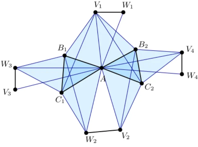
• two vertices Vj and Wj and the edge VjWj for each variable vj. W4 W3 W6 W1 W2 W5 B4 C3 B2 C1 B1 C2 B3 A V1 V2 V3 V4 V5 V6 C5 B5 C4
Figure 8: Simplicial complex L output by the reduc-tion of a formula with five clauses and six variables and triangles in K created by clause c1= v2∨¬v3∨¬v5.
Besides simplices in L, the simplicial complex K contains three triangles per literal and two edges per variable. Specif-ically, if ek
i = 1, we add the three triangles ABiVjk
i, BiCiVjik and CiAVjk
i and their edges. If e k
i =¬, we add the three triangles ABiWjk
i, BiCiWjki and CiAWjik and their edges. Moreover, we add edges AVjand AWjfor all j∈ {1, . . . , m}. Observe that the size of K is only a constant factor larger than the size of E and its construction requires linear time in n. B1 V1 W1 B2 A C1 W2 V2 C2 W4 V4 W3 V3
Figure 9: Pair (K, L) produced by the reduction of formula (v1∨ ¬v2∨ ¬v3)∧ (v1∨ v2∨ v4). L consists of the vertices and bold edges.
Let f∗: Hp(L)→ Hp(K) be the homomorphism induced by the inclusion L ⊂ K. Since K is connected, we have f∗(H0(L)) = Z2. Furthermore, f∗(H1(L)) = 0 since a base of the 1-cycles in L is given by the n cycles σi= ABi+BiCi+ CiA and σiis homologous to 0 in K for each i∈ {1, . . . , n}. Last, f∗(H2(L)) = 0 since L contains no 2-simplices. By Lemma 7, we obtain that X is a homological simplification of the pair (K, L) if and only if H0(X) = Z2, H1(X) = 0 and H2(X) = 0. Keeping this in mind, we establish the
following lemma, in which (K, L) designates the pair output by our reduction algorithm when applied to formula E.
Lemma 9. The pair (K, L) has a homological simplifica-tion if and only if the formula E has a satisfying assignment. Furthermore, given a homological simplification of the pair (K, L), computing a satisfying assignment for E takes linear time.
Proof. Suppose the pair (K, L) has a homological sim-plification X and let us prove that E has a satisfying assign-ment. First, we claim that X cannot contain both edges AVj and AWj, for 1 ≤ j ≤ m. Indeed, if both edges AVj and AWj were in X, we could consider the cycle τ = AVj+ VjWj+ WjA. Since the edge VjWj bounds no tri-angle in K, the cycle τ cannot be homologous to 0 in X, contradicting H1(X) = 0.
The claim allows us to assign to each variable vjeither the value TRUE if the edge AVjbelongs to X or the value FALSE if the edge AWjbelongs to X. If none of the edges AVjand AWjbelong to X, then we assign to vjan arbitrary value in {TRUE, FALSE}; see Figure 10. Note that the computation of this assignment can be done in linear time. We now check that this assignment of boolean values to the variables vj is a satisfying assignment, in other words we show that all clauses ciare satisfied for 1≤ i ≤ n.
Since H1(X) = 0, the 1-cycle ABi+ BiCi+ CiA is a boundary in X. This implies that at least one triangle of X contains ABion its boundary. By construction, ABibelongs to exactly three triangles in K, namely the triangles ABiYk i for 1≤ k ≤ 3 where Yk i designates Vjk i if e k i = 1 and Wjk i if ek
i =¬. It follows that one of the three triangles ABiYik must belong to X and, in turn, at least one of the three edges AYik for 1 ≤ k ≤ 3 is in X. This implies that one of the three literals ekivjk
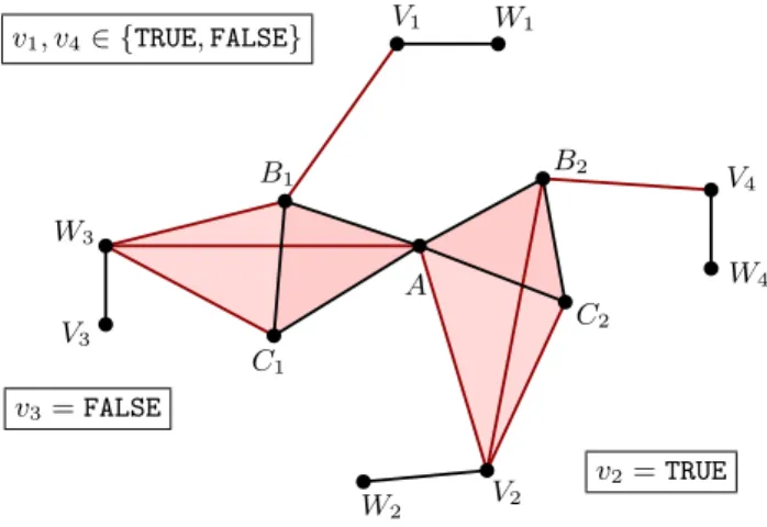
i in clause cievaluates to TRUE and hence ciis satisfied. v3= FALSE v1, v4∈ {TRUE, FALSE} v2= TRUE W3 V1 W1 B2 C1 W2 V2 C2 W4 V4 V3 B1 A
Figure 10: A homological simplification of the pair (K, L) drawn in Figure 9 and output by the reduc-tion of formula E = (v1∨ ¬v2∨ ¬v3)∧ (v1∨ v2∨ v4). Corresponding satisfying assignments for E.
Conversely, suppose variables v1, . . . , vm have been as-signed values that cause E to evaluate to TRUE and let us prove that the pair (K, L) has a homological simplification X. We construct X starting from L and adding some sim-plices of K as follows; see Figure 11. We begin by adding
the edge AVjif vj= TRUE and the edge AWjif vj= FALSE, for all j∈ {1, . . . , m}. Since values of v1, . . . , vmare a sat-isfying assignment, we can choose one literal eivji in each clause cithat is true. Let Yi= Vjiif ei= 1 and Yi= Wji if ei=¬. Note that by construction, the edge AYi is already in X. We then add the three triangles ABiYi, BiCiYi and CiAYi to X, for all i∈ {1, . . . , n}.
v2= FALSE v3= TRUE v1= FALSE v4= TRUE W3 B1 A V1 W1 B2 V4 W4 C2 V2 W2 C1 V3
Figure 11: Satisfying assignment for formula E = (v1∨ ¬v2∨ ¬v3)∧ (v1∨ v2∨ v4) and corresponding ho-mological simplification of (K, L).
Let us check that X is indeed a solution to the homological simplification problem, i.e. H0(X) = Z2, H1(X) = 0 and H2(X) = 0. For this, we check that X is contractible by collapsing X to A, using a sequence of elementary collapses. First, observe that exactly one of the two vertices Vj or Wj belongs to no other simplices than the edge VjWj. For instance, if vj = TRUE, then by construction AVj ∈ X and AWj 6∈ X. Thus, Wj belongs to no other simplices than VjWj and we can collapse the edge VjWj to the vertex Vj by removing the pair of simplices (Wj, VjWj). Similarly, if vj= FALSE, we collapse the edge VjWjto the vertex Wj. For all i ∈ {1, . . . , n}, we apply five elementary collapses, first removing the three triangles ABiYi, BiCiYiand CiAYiand their edges ABi, BiCi and CiA, then removing the edges BiYi and CiYiand their vertices Bi and Ci. In a last step, we collapse every edge AYifor 1≤ i ≤ n to the vertex A.
4.
DISCUSSION
Our work raises several questions and research tracks.
Open questions.
Is there a version of Lemma 6 in which the voxel size does not depend on µ? Is the homological simplification problem in the same class of complexity if we constraint K to be a subcomplex of a triangulation of the sphere S3?
Optimistic research track.
If a polynomial time optimal reconstruction algorithm ex-ists, it should take advantage of the embedding in Euclidean space or at least lead to a class of simplification problems suf-ficiently constrained to avoid constructions similar to ours.
Pessimistic research track.
Is it possible to encode 3-SAT as the homological simplifi-cation of a pair (K3α(S), Kα(S)), where (S, α) satisfies the weak sampling condition? Or, as the homological simplifica-tion of a pair of cubical complexes defined by offsets of the sample? If yes, in which minimal dimension?
5.
REFERENCES
[1] N. Amenta and M. Bern. Surface reconstruction by Voronoi filtering. Discrete and Computational Geometry, 22(4):481–504, 1999.
[2] N. Amenta, M. Bern, and D. Eppstein. The crust and the β-skeleton: Combinatorial curve reconstruction. Graphical Models and Image Processing,
60(2):125–135, 1998.
[3] N. Amenta, S. Choi, T. Dey, and N. Leekha. A simple algorithm for homeomorphic surface reconstruction. In Proceedings of the sixteenth annual symposium on Computational geometry, pages 213–222. ACM New York, NY, USA, 2000.
[4] N. Amenta, S. Choi, and R. Kolluri. The power crust, unions of balls, and the medial axis transform. Computational Geometry: Theory and Applications, 19(2-3):127–153, 2001.
[5] D. Attali. r-regular shape reconstruction from unorganized points. Computational Geometry: Theory and Applications, 10:239–247, 1998.
[6] D. Attali, M. Glisse, S. Hornus, F. Lazarus, and D. Morozov. Persistence-sensitive simplification of functions on surfaces in linear time. Manuscript, INRIA, 2008.
[7] D. Attali and A. Lieutier. Reconstructing shapes with guarantees by unions of convex sets.
http://hal.archives-ouvertes.fr/hal-00427035/en/. [8] D. Attali and A. Lieutier. Reconstructing shapes with
guarantees by unions of convex sets. In Proc. ACM Symposium on Computational Geometry, 2010. Submitted.
[9] J. Boissonnat and F. Cazals. Smooth surface reconstruction via natural neighbour interpolation of distance functions. Computational Geometry: Theory and Applications, 22(1-3):185–203, 2002.
[10] J. Boissonnat, L. Guibas, and S. Oudot. Manifold reconstruction in arbitrary dimensions using witness complexes. Discrete and Computational Geometry, 42(1):37–70, 2009.
[11] J. Boissonnat and S. Oudot. Provably good sampling and meshing of Lipschitz surfaces. In Proceedings of the twenty-second annual symposium on
Computational geometry, page 346. ACM, 2006. [12] F. Chazal, D. Cohen-Steiner, and A. Lieutier. A
sampling theory for compact sets in Euclidean space. Discrete and Computational Geometry, 41(3):461–479, 2009.
[13] F. Chazal, D. Cohen-Steiner, A. Lieutier, and B. Thibert. Shape smoothing using double offsets. In Proc. of the ACM symposium on Solid and physical modeling, pages 183–192. ACM New York, NY, USA, 2007.
[14] F. Chazal and A. Lieutier. Stability and computation of topological invariants of solids in Rn. Discrete and Computational Geometry, 37(4):601–617, 2007.
[15] F. Chazal and S. Oudot. Towards persistence-based reconstruction in Euclidean spaces. In Proceedings of the twenty-fourth annual symposium on
Computational geometry, pages 232–241. ACM, 2008. [16] F. Clarke. Optimization and nonsmooth analysis.
Society for Industrial Mathematics, 1990. [17] D. Cohen-Steiner. Personal communication. 2008. [18] D. Cohen-Steiner, H. Edelsbrunner, and J. Harer.
Stability of persistence diagrams. Discrete and Computational Geometry, 37(1):103–120, 2007. [19] T. Cormen, C. Leiserson, R. Rivest, and C. Stein.
Introduction to algorithms, 2001.
[20] V. de Silva. Personal communication. 2009.
[21] V. de Silva and G. Carlsson. Topological estimation using witness complexes. Proc. Sympos. Point-Based Graphics, pages 157–166, 2004.
[22] T. Dey, S. Funke, and E. Ramos. Surface reconstruction in almost linear time under locally uniform sampling. In Abstracts 17th European Workshop Comput. Geom, pages 129–132. Citeseer, 2001.
[23] T. Dey, J. Giesen, E. Ramos, and B. Sadri. Critical points of the distance to an epsilon-sampling of a surface and flow-complex-based surface reconstruction. In Proc. of the twenty-first annual symposium on Computational geometry, page 227. ACM, 2005. [24] T. Dey and S. Goswami. Provable surface
reconstruction from noisy samples. Computational Geometry: Theory and Applications, 35(1-2):124–141, 2006.
[25] T. Dey and K. Li. Cut locus and topology from surface point data. In Proceedings of the 25th annual symposium on Computational geometry, pages 125–134. ACM New York, NY, USA, 2009. [26] H. Edelsbrunner, D. Letscher, and A. Zomorodian.
Topological persistence and simplification. Discrete and Computational Geometry, 28(4):511–533, 2002. [27] H. Edelsbrunner, D. Morozov, and V. Pascucci.
Persistence-sensitive simplification functions on 2-manifolds. In Proceedings of the twenty-second annual symposium on Computational geometry, page 134. ACM, 2006.
[28] K. Grove. Critical point theory for distance functions. In Proc. of Symposia in Pure Mathematics, volume 54, pages 357–386, 1993.
[29] A. Lieutier. Any open bounded subset of R n has the same homotopy type as its medial axis.
Computer-Aided Design, 36(11):1029–1046, 2004. [30] D. Morozov. Homological Illusions of Persistence and
Stability. Ph.D. Dissertation, Duke University, 2008. [31] J. Munkres. Elements of algebraic topology. Perseus
Books, 1993.
[32] P. Niyogi, S. Smale, and S. Weinberger. Finding the Homology of Submanifolds with High Confidence from Random Samples. Discrete Computational Geometry, 39(1-3):419–441, 2008.
[33] S. Oudot. ´Echantillonnage et maillage de surfaces avec garanties. Ph.D. Dissertation, Ecole Polytechnique, 2005.
APPENDIX
This appendix establishes the correctness of our first naive reconstruction algorithm. First, we establish the existence of cubical sets that are faithful reconstruction of shapes with positive µ-reach, using Corollary 3 in [7]:
Lemma 10 (Corollary 3 in [7]). For dN = 1 40N3⌈√N ⌉ and for all compact setsA ⊂ RNwith reach greater than ρ > 0, there exists a (dNρ)-cubical setX such that A ⊂ X ⊂ Aρ and the inclusion mapsA ֒→ X and X ֒→ Aρare homotopy equivalences.
Proof of Lemma 6. The proof of Lemma 6 consists in extending the above lemma to the situation where compact sets have a positive µ-reach with the constant cN = dN
2 . Given a setY ⊂ RN, we denote respectively by
Y and Yc the closure and the complement ofY. For any compact set X ⊂ RN and any real number ρ > 0, let
X−ρ = ((Xc)ρ)c and consider the setB = (Ay)−µ(y−x). We know from [13] that the reach ofB is greater than or equal to µ(y − x) and the inclusion maps corresponding to the sequence
Ax ⊂ B ⊂ Ay
are homotopy equivalences. We can now apply Corollary 3 in [7] to the setB whose reach is greater than ρ = µ(y−x)2 . This gives the existence of a (cNµ(y− x))-cubical set X such that:
B ⊂ X ⊂ Bρ
and the maps corresponding to inclusions are homotopy equiv-alences. UsingBρ= ((
Ay)−2ρ)ρ
⊂ Ay, we get the sequence of inclusions
Ax ⊂ X ⊂ Ay. in which the inclusion mapAx֒
→ X is a homotopy equiva-lence. By Lemma 2,X is a faithful reconstruction of A.
Under precondition 3, next lemma states the existence of a cubical set which is a faithful reconstruction nested between two cubical sets that can be deduced from the sample (see Figure 4). Given a compact subsetY ⊂ RN, we recall that Vε(Y) designates the union of ε-voxels that intersect Y. The underlying space of the simplicial complex X is denoted|X|. Lemma 11. Let α, η > 0 and µ ∈ (0, 1] be real num-bers and let A and S be compact subsets of RN such that dH(S, A) < α <1 4(rµ(A) − η). Then, for: ε = η 4√N + 2 cNµ , l = η 2+ α, k = η + 3α− ε √ N , there exists an ε-cubical setX such that:
Aη2 ⊂ Vε(Sl) ⊂ X ⊂ Vε(Sk) ⊂ Aη+4α
and the inclusion maps Aη2 ֒→ X and X ֒→ A4α+η are homotopy equivalences. In particular,X is a faithful recon-struction ofA. Furthermore, if we have three nested simpli-cial complexes L⊂ X ⊂ K such that Vε(Sl) =|L|, X = |X| and Vε(Sk) =
|K|, then X is a homological simplification of the pair (K, L).
Proof. Note that for all compact setY ⊂ RN, we have Y ⊂ Vε(Y) ⊂ Yε√N. It follows that for all t
≥ 0, we have the following sequence of inclusions:
At ⊂ St+α ⊂ Vε(St+α) ⊂ St+α+ε √ N ⊂ At+2α+ε √ N.
Applying this sequence twice, once for t = η2 and once for t = η + 2α− ε√N , we get that Aη2 ⊂ Vε(S η 2+α) ⊂ A η 2+2α+ε √ N ⊂ Aη+2α−ε√N ⊂ Vε(Sη+3α−ε√N) ⊂ Aη+4α. The value ε has been chosen precisely such that the pa-rameters of the two offsets ofA in the middle differ by ε
cNµ. Specifically, writing x = η 2+2α+ε √ N and y = η+2α−ε√N , we have y−x = ε
cNµ. Hence, applying Lemma 6 toA, we get the existence of an ε-cubical setX such that Ax
⊂ X ⊂ Ay and the maps corresponding to the inclusions are homotopy equivalences. The first part of the lemma follows. For the second part, notice that we have the following sequence of homomorphisms induced by inclusion maps:
Hp(Aη2)→ Hp(|L|) → Hp(|X|) → Hp(|K|) → Hp(Aη+4α). We will use the following observation. Consider two func-tions i : E→ F and j : F → G such that the composition j◦i is bijective. Then, i is injective and j is surjective. Since the map Hp(Aη2)→ Hp(|X|) induced on homology groups by inclusion is bijective, the map Hp(|L|) → Hp(|X|) is sur-jective using the observation. Similarly, the map Hp(|X|) → Hp(|K|) is injective and therefore X is a homological sim-plification of the pair (K, L).
Lemma 12. Let x1, x2, x3 be real numbers andA a com-pact subset of RN such that 0 < x1 < x2 < x3 < wfs(A). Let L⊂ K be two simplicial complexes such that:
Ax1
⊂ |L| ⊂ Ax2
⊂ |K| ⊂ Ax3
If X is a homological simplification of the pair (K, L), then |X| is a faithful homological reconstruction of A.
Proof. Inclusion maps induce the following commuta-tive diagram between homology groups:
Hp(Ax2) Hp(Ax1) >Hp( |L|) > Hp(|K|) > > Hp(Ax3) Hp(|X|) > >
From Lemma 1, the maps Hp(Ax1)
→ Hp(Ax2)→ Hp(Ax3) are isomorphisms. Since we take coefficients in a field, ho-mology groups are vector spaces. Since the map Hp(Ax1)
→ Hp(Ax2) induced by inclusion is bijective, the map Hp(
|L|) → Hp(Ax2) is surjective. Since Hp( Ax2) → Hp(Ax3) is bi-jective, Hp(Ax2) → H p(|K|) is injective. By an argu-ment similar to the one used in the proof of Lemma 7, we deduce that the dimensions of Hp(Ax2) and Hp(
|X|) are equal to the rank of Hp(|L|) → Hp(|K|) and there-fore dim Hp(|X|) = dim Hp(Axi) for all 1 ≤ i ≤ 3. Since Hp(Ax1)
→ Hp(Ax3) is bijective, Hp(Ax1)→ Hp(|X|) is injective. Because its domain and image have same dimen-sion, it follows that Hp(Ax1)
→ Hp(|X|) is an isomorphism. Similarly Hp(|X|) → Hp(Ax3) is an isomorphism and |X| is a faithful homological reconstruction ofA.