Combination of frequency shift and impedance-based method for robust temperature sensing using piezoceramic devices for shm

HAL Id: hal-01620039

https://hal.archives-ouvertes.fr/hal-01620039

HAL is a multi-disciplinary open access

archive for the deposit and dissemination of sci-entific research documents, whether they are pub-lished or not. The documents may come from teaching and research institutions in France or abroad, or from public or private research centers.

L’archive ouverte pluridisciplinaire HAL, est destinée au dépôt et à la diffusion de documents scientifiques de niveau recherche, publiés ou non, émanant des établissements d’enseignement et de recherche français ou étrangers, des laboratoires publics ou privés.

Combination of frequency shift and impedance-based

method for robust temperature sensing using

piezoceramic devices for shm

Emmanuel Lizé, Charles Hudin, Nicolas Guenard, Marc Rébillat, Nazih

Mechbal, Christian Bolzmacher

To cite this version:

Emmanuel Lizé, Charles Hudin, Nicolas Guenard, Marc Rébillat, Nazih Mechbal, et al.. Combination of frequency shift and impedance-based method for robust temperature sensing using piezoceramic devices for shm. EWSHM 2016, Jul 2016, Bilbao, Spain. �hal-01620039�

COMBINATION OF FREQUENCY SHIFT AND IMPEDANCE-BASED

METHOD FOR ROBUST TEMPERATURE SENSING USING

PIEZOCERAMIC DEVICES FOR SHM

Emmanuel LIZE1, Charles HUDIN1, Nicolas GUENARD1, Marc REBILLAT2, Nazih MECHBAL2, Christian BOLZMACHER1

1 _{CEA, LIST, Sensorial and Ambient Interfaces Laboratory, 91191 - Gif-sur-Yvette CEDEX, France;}

2 _{Processes and Engineering in Mechanics and Materials Laboratory (PIMM, UMR CNRS}

8006, Arts et Métiers ParisTech (ENSAM)), 151, Boulevard de l'Hôpital, Paris, F-75013, France; emmanuel.lize@cea.fr

Key words: guided waves (lamb waves), Piezoelectric sensors, composite, temperature, impedance, frequency-shift, SHM.

Abstract

The influence of temperature is a major problem in Structural Health Monitoring diagnosis using guided waves. In this article, two methods for temperature compensation are used to evaluate the temperature of a structure monitored by Piezoceramic Transducers (PZT). The first one consists in a linear regression of the static capacity of the PZT (computed with the electromechanical impedance) with the temperature. It allows one to determine temperature of a PZT from any impedance measurement. The second method is based on the Modes Frequency Shift (MFS) of the frequency response function (FRF) calculated in a pitch-catch mode with an exponential sweep signal. A linear regression between the MFS and the temperature is settled for most modes and allow the estimation of temperature between two PZT. Experiments on a composite plate monitored by 5 PZT patches showed that a ±2°𝐶 variation can easily be identified with both methods. Combined together, those two methods could replace actual temperature sensors and bring an efficient improvement for temperature compensation in applications where the temperature variation is heterogeneous on a structure.

1 INTRODUCTION

Structural Health Monitoring (SHM) is a field that has been continuously evolving for the last 20 years. The revolution of new technologies and improvements in computer science leads to great innovations on existing techniques, such as signal processing, that allow one to create more complex methods and bring more accurate results in SHM. However, some important parameters are still difficult to handle, including the influence of environmental conditions and the complexity of materials of monitored structures. The aerospace industry is specifically concerned by these technological improvements since composite materials tend to replace aluminum and the maintenance becomes quite expensive.

Damage detection using guided waves is one of the most used methods in SHM. The ultrasonic wave propagation in a structure is altered by the material properties, the geometry and the presence of damages. Among all the methods employed to trigger and catch guided waves, the use of piezoelectric transducer (PZT) is one of the cheapest and easiest-to-settle.

2

The study of electromechanical signature of PZT devices has gained importance in the SHM community [1]–[3]. It consists in measuring the impedance of PZT coupled with a structure under test. This method can be used as a damage-detection method and to evaluate a PZT boundary condition or health degradation. It has shown very good results under laboratory conditions and has already been deployed under real-life conditions. In an aeronautical context, the influence of temperature variations on the impedance of surface-mounted PZT is not negligible and has been the focus of several research teams. Experimental [4]–[6] as well as numerical studies [7], [8] pointed out that the static capacity of a PZT increases, and the modal frequencies are lowered when the temperature rises [9]– [11]. Those observations have led to temperature compensation methods, and efforts have been made to distinguish modifications attributable to temperature from modifications due to damage [10]–[13]. All the studies are efficient in proving the sensibility of PZT to temperature, but to the authors’ knowledge, very few works have been carried out in order to use the PZT as a temperature sensor using static capacity. Ilg & al. [14] demonstrated that it is possible to use an air ultrasound transducer to estimate the air temperature with a ±4.5°𝐶 accuracy using the static capacity of PZT at 1kHz. Yet, this study didn’t show results of surface mounted PZT.

Since wave propagation in structures is used in SHM, its sensibility to temperature variation has been investigated in numerous studies [15], [16]. It has been demonstrated that changes of properties and geometry of the structure being caused by temperature variations are one of the environmental parameters that reduces the most significantly the probability of detection of damages in a structure [17]. Many studies exist on homogenous structures such as aluminum plates, but fewer work has been applied to composite structures as Carbon Fiber Reinforced Plastic (CFRP). However, some effective temperature-compensation models already exist. Those methods are mostly based on time domain measures [18] or their interpretation in the frequency domain. For example, Crowford & al. [19], [20] introduced the Optimal Baseline Selection (OBS) and the Baseline Signal Stretch (BSS) in the time domain. Clarke et al. [21] used the same methods in the frequency domain. The combination of those 2 techniques is effective and enables to have smaller baselines. More complex algorithms have been developed using this combination [22]. The main influence of temperature on the frequency response function (FRF) resides in a variation of the modal damping and a frequency shift of the modal resonances. This observation is used for temperature compensation (BSS in the frequency domain) but has never been used to propose a way to determine the temperature of the structure between an actuator-sensor couple.

This article is organized as follows. The static capacity and the modal frequency-shift temperature identification methods are first described. Then the experimental set-up used to study the influence of temperature and the effectiveness of the proposed identification methods is presented. Finally, experimental results are displayed.

2 STATIC CAPACITY AND MODAL FREQUENCY SHIFT

This section defines the static capacity of a PZT mounted on a structure and how it can be used to determine temperature. It also presents the frequency response function (FRF) obtained with an exponential sweep and how the frequency shift of the observed modes can be used to evaluate the temperature. Eventually, two indicators are described: the coefficient of determination and the error of temperature estimation.

3 2.1 Static capacity computation

A PZT mounted on a structure can be qualified by its electro-mechanical signature. The impedance 𝑍(𝑓) and its inverse, the admittance 𝑌(𝑓), are defined as the transfer function between voltage 𝑉(𝑓) applied to the PZT element and the resulting current 𝐼(𝑓)The equivalent capacity at a given frequency 𝐶(𝑓) is defined as the absolute value of the admittance divided by 2𝜋𝑓. The variable 𝑓 denotes the frequency.

𝐶(𝑓) = |𝑌(𝑓) 2𝜋𝑓 | 𝑤ℎ𝑒𝑟𝑒 𝑌(𝑓) = 1 𝑍(𝑓) = 𝐼(𝑓) 𝑉(𝑓) (1)

The static capacity is the mean of the equivalent capacity computed on a range of frequencies from 𝑓_𝑎 to 𝑓_𝑏: 𝐶_𝑠 = 1 𝑓_𝑏− 𝑓_𝑎∫ 𝐶(𝑓)𝑑𝑓 𝑓𝑏 𝑓𝑎 (2)

2.2 Estimation of the temperature using static capacity

Variations of temperature have a non-negligible effect on material properties of the structure under test, the PZT and the bounding. As a matter of fact, the static capacity of a PZT increases as the temperature rises and decreases as the temperature drops.

Experiments on a CFRP plate subject to temperature variation cycles between 0 and 80°C allow us to propose a linear regression of the static capacity with temperature:

𝐶𝑠(𝜃) = 𝛼𝐶× 𝜃 + 𝐶𝑠0 (3)

The variables 𝛼𝐶 and 𝐶𝑠0 are respectively the temperature variation coefficient and the

static capacity at 0°C. They are determined using experimental data acquisition of static capacity measurements. The variation of static capacity ∆𝐶_𝑠(𝜃) is also defined as:

∆𝐶_𝑠(𝜃) = 𝐶_𝑠(𝜃) − 𝐶_𝑠0 _{= 𝛼} 𝐶× 𝜃

Therefore, an estimation of the temperature of a PZT mounted on a structure 𝜃̂_{𝑒𝑠𝑡𝑖𝑚} can be calculated with the variation of static capacity for any measurement ∆𝐶_{𝑠,𝑚𝑒𝑠}:

𝜃̂_{𝑒𝑠𝑡𝑖𝑚} = ∆𝐶𝑠,𝑚𝑒𝑠

𝛼_𝐶 (4)

2.3 FRF using an exponential sweep signal

The exponential sweep signal is used to excite all the modes of the structure under test within a programed range of frequencies. Compared to other excitation signals composed of multiple sines (random multisine, linear sweep), the exponential sweep signal is more robust to non-linearities and less sensitive to distributed noises [23]. The FRF is the transfer function 𝐻(𝜔) which corresponds to the cross power spectral density of the signal recorded by the PZT sensor and the signal emitted by the PZT actuator divided by the power spectral density of the signal emitted by the PZT actuator. It is equivalent to the following equation:

𝐻(𝜔) = 𝑉(𝜔) × 𝑈(𝜔)

|𝑈(𝜔)|² (5)

where 𝑉(𝜔) and 𝑈(𝜔) are the Fourier transform of the signal recorded by the PZT sensor and the signal emitted by the PZT actuator. The modes 𝑟 refer to the peaks observed in the

4

FRF. They are defined by their pulsation at temperature 𝜃 by 𝜔𝑟(𝜃) in Hertz.

2.4 Influence of temperature on the FRF

The modal-frequency-shift (MFS) is the frequency variation of modes observed when the temperature changes. Its variation ∆𝜔_𝑟 is estimated by

∆𝜔𝑟(𝜃) = 𝜔𝑟(𝜃) − 𝜔𝑟0 (6)

where 𝜔𝑟0 is the pulsation of the mode 𝑟 at 0°C.

In previous studies using FRF it has been noticed that the MFS towards lower frequencies increases for higher frequency and for rising temperature. For the first experiments, two main assumptions have been made concerning the MFS evolution:

i. The MFS of each mode is linear with temperature

ii. No regression model is applied regarding the MFS variation with frequency. The thermal drift coefficient 𝛼_𝑟 of a given mode 𝑟 satisfies the relation

∆𝜔𝑟(𝜃) = 𝛼𝑟× 𝜃 (7)

It is important to notice that 𝛼𝑟 corresponds to one specific mode. 𝛼𝑟 and 𝜔𝑟0 are

determined using experimental data of FRF acquisitions. 2.5 Temperature estimation using the FRF

Using Eq.(7), the temperature of any FRF measurement can be estimated from the MFS measured for a given mode ∆𝜔_{𝑟,𝑚𝑒𝑠}:

𝜃̂_{𝑟,𝑒𝑠𝑡𝑖𝑚} =∆𝜔𝑟,𝑚𝑒𝑠

𝛼_𝑟 (8)

The use of a broadband signal allows the exploitation of several modes. It leads to a more robust result of the estimated temperature.

For 𝑁 considered modes, the mean of the estimated temperature 𝜃̅̅̅̅̅̅̅̅ is computed 𝑒𝑠𝑡𝑖𝑚

iteratively by minimizing the standard deviation 𝜎, as described below. The final value of the mean calculated corresponds to the estimated temperature 𝜃̂_{𝑒𝑠𝑡𝑖𝑚}.

Algorithm 1: Temperature estimation with 𝑁 modes.

Calculate: 𝜃̂_{𝑒𝑠𝑡𝑖𝑚} = 𝜃̅_{𝑒𝑠𝑡𝑖𝑚} = ∑𝑟=𝑁𝑟=1𝜃̂𝑟,𝑒𝑠𝑡𝑖𝑚

𝑁 and 𝜎 = √

∑𝑟=𝑁𝑟=1[𝜃̂𝑒𝑠𝑡𝑖𝑚(𝑟)−𝜃̅𝑒𝑠𝑡𝑖𝑚 ]

𝑁

while ∃𝜃̂𝑟,𝑒𝑠𝑡𝑖𝑚∉ [𝜃̅𝑒𝑠𝑡𝑖𝑚 ∓ 𝜎]

𝐷𝑜 for each 𝑟, delete 𝑟 if 𝜃̂𝑟,𝑒𝑠𝑡𝑖𝑚 ∉ [𝜃̅𝑒𝑠𝑡𝑖𝑚 ∓ 𝜎]

compute 𝑁, 𝜃̅_{𝑒𝑠𝑡𝑖𝑚} and 𝜎 with the remaining 𝑟 end while

𝜃̂𝑒𝑠𝑡𝑖𝑚 = 𝜃̅𝑒𝑠𝑡𝑖𝑚

2.6 Indicators

The coefficient of determination 𝑟² is used as an indicator for linear regression verification. It is between 0 (erroneous linear regression) and 1 (perfect fit).

The error of estimation 𝜀_𝜃 is the absolute value of the difference between the estimated temperature 𝜃_{𝑒𝑠𝑡𝑖𝑚} and the measured temperature 𝜃_{𝑚𝑒𝑎𝑠}:

5 3 EXPERIMENTS AND RESULTS

This section describes the setup used for the experiments and results obtained for temperature estimation with both methods (static capacity and MFS).

3.1 Structure under test and protocols

The testing was performed on a 400 𝑚𝑚 × 300 𝑚𝑚 CFRP plate of 4 plies [0/−45/45/ 0]. Each ply is 0.28 𝑚𝑚 thick. This structure is instrumented with 5 Noliac NCE51 piezoceramics transducers with a diameter of 20 𝑚𝑚, a thickness of 0.5 𝑚𝑚 and a Curie temperature of 360°𝐶. Each PZT can be used as an actuator or a sensor. All the PZT were mounted on the structure with the glue Redux 322. According to the manufacturer data sheet, this glue can be used between −55°𝐶 and 200°𝐶.

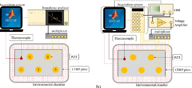
Impedance and FRF measurements were done at the same time. The CFRP plate was placed in an environmental chamber where the temperature could be controlled between −60°𝐶 and 120°𝐶 (WEISS WKL100). A type K thermocouple was placed on the plate and acquired with a NI 9213 data acquisition card. A multiplexor AGILENT L4421 was used to switch PZT actuator/sensor or Impedance/FRF measurement. The acquisition system was monitored using Matlab. Impedance measurements were realized with a Hioki IM3570 impedance analyzer (see Figure 1.a). At each temperature of a cycle, the impedance measurement of PZTs was acquired three times with 800 points between 20 𝑘𝐻𝑧 and 60 𝑘𝐻𝑧. These measurements were then averaged in the frequency domain in order to increase the signal to noise ratio (SNR).

For FRF measurements, the exponential sweep signal was emitted with a waveform generator (Agilent 33500 Arbitrary Waveform Generator) and a voltage amplifier (see Figure 1.b). The signal recorded by the PZT sensor was acquired with a Genesis GEN7t card. The emitted signal for each measurement is a 10 𝑚𝑠 exponential sweep from 10 𝑘𝐻𝑧 to 250 𝑘𝐻𝑧 with a sampling frequency of 100 𝑀𝐻𝑧.The response signal of the PZT sensor elements was recorded during 15 𝑚𝑠 with a sampling frequency of 1 𝑀𝐻𝑧and averaged 100 times to minimize the SNR.

The FRF (see Eq.(5)) was calculated using the Matlab function tfestimate.m.

a) b)

6 3.2 Impedance measurements

Creation of the database

The database was realized with capacity measurements on a cycle (increase/decrease) from 10°𝐶 to 60°𝐶 by step of 2°𝐶. It is composed of the parameters of the linear regression described in Eq. (3): the static capacity variation coefficient 𝛼_𝐶 and the static capacity at 0°𝐶, 𝐶𝑠0, for each PZT considered. Figure 2 shows the evolution of the static capacity

measurements used to create the database for PZT 1. It confirms that the static capacity variation is proportional to the temperature. A hysteresis effect is observed when the temperature variation changes direction. However, this phenomenon will not be taken into account in this article (unlike [14]) but may be studied in future works. Figure 2a indicates that a smaller range of frequencies or even one frequency can be used to determine the temperature variation, but considering a larger scope increases the robustness of the results.

a) b)

Figure 2 : a) variation of the equivalent capacity described in Eq. (1) of PZT 1 with temperature on the range 20 to 60 kHz, b) variation of the static capacity described in Eq. (2) of PZT 1 on the temperature cycle used

as baseline and linear regression computed

PZT1 PZT 2 PZT 3 PZT 4 PZT 5

𝛼𝐶 (× 10−11𝐹/°𝐶) 1.60 1.56 1.81 1.54 1.57

𝐶𝑠0 (𝑛𝐹) 6.67 6.60 7.13 6.65 6.88

𝑟² 0.99 0.95 0.94 0.99 0.99

Table 1: linear regression parameters and coefficient of determination of the capacity variation with temperature for the 5 PZT of the structure under test

The linear regression is estimated (Figure 2b) and stored as a reference in the database: The parameters are slightly different despite the fact that all the PZT are of the same material and are mounted in the same way. This difference can come from PZT health degradation due to previous tests and also differences in the acquisition system (for example, cables are not exactly the same length).

Temperature estimation

A second cycle from 0 to 80°𝐶 and from 80°𝐶 to 62°𝐶 by steps of 2°𝐶 was used as a test sample for temperature estimation. The temperature is estimated using Eq. (4).

7

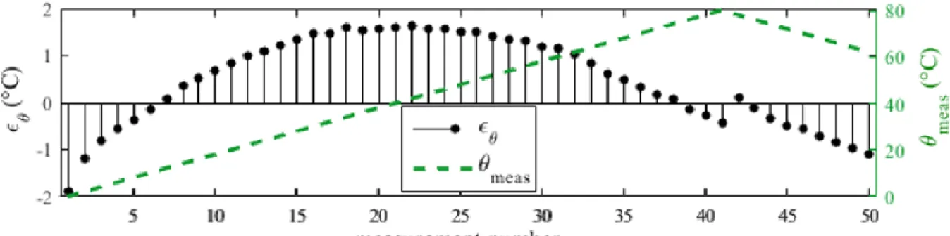
Figure 3: error in the temperature estimation by impedance for 50 test measurements with PZT 1

The error of estimation 𝜀_𝜃 (Eq.(9)) indicates a precision of ±2°𝐶 of the temperature measurement using the static capacity of PZT 1. PZT 2 and 4 had the same precision (±2°𝐶), but PZT 3 and 5 showed poorer results (respectively ±10°𝐶 and ±5°𝐶). For the moment, experiments have only been made with temperatures from 0 to 80°𝐶 on one undamaged CFRP plate and showed good results. Further tests on other CFRP structures and with more extreme temperatures will approve the model and delimit its application range. Figure 2a shows a tendency of the capacity to shift under lower frequencies with increasing temperature. This observation might be used for further development to improve the current method.

3.3 FRF measurements

Creation of the database

a) b)

c)

Figure 4: a) MFS of the mode at 136.9 kHz. The triangle represents the position of the peak; b) linear

regression applied on the MFS variation of the mode at 136.9kHz (𝛼𝑟= −37 𝐻𝑧/°𝐶; 𝜔𝑟0= 136.9 𝑘𝐻𝑧); c)

FRF of path PZT1 - PZT 2 for temperatures varying from 10 to 60°C (top) and thermal drift coefficient for the 80 modes considered (bottom)

8

The modes are tracked with the Matlab function findpeaks.m. An algorithm has been developed in order to follow the MFS that occurs with temperature variations (Figure 4a). This work focuses on the position of the modal pulsation but other parameters like damping and amplitude could be considered in future works. The database was realized with FRF measurements on a cycle (increase/decrease) from 10°𝐶 to 60°𝐶 by steps of 2°𝐶. It is composed of the parameters of the linear regression described in Eq. (6) and (7): the thermal drift coefficient 𝛼_𝑟 and the pulsation frequency at 0°𝐶 𝜔_𝑟0 _{for each mode 𝑟 and for each PZT}

are considered. Variables 𝛼𝑟 and 𝜔𝑟0 are determined by studying the MSF of each mode on

the cycle used as reference. Figure 4b shows the linear regression applied to the mode at 136.9 𝑘𝐻𝑧 in order to determine 𝛼𝑟 and 𝜔𝑟0. The MSF corresponding to the rising in

temperature from 10°𝐶 to 60°𝐶 of this same mode is displayed in Figure 4a.

For each mode, the coefficient of determination is computed. It is an important parameter to confirm the validity of the proposed linear regression. The FRF modes are chosen between 10 𝑘𝐻𝑧 and 190 𝑘𝐻𝑧 (for frequencies higher than 190 𝑘𝐻𝑧, the peaks corresponding to mode pulsations are difficult to follow upon temperature variation). Considering this range, 80 modes are detected and their parameters are recorded in the database. The coefficient of determination calculated for the 80 modes are between 0.4 and 1 with a mean of 0.94. This result proves that the linear regression is a good model for the variation of the MSF with temperature. As discussed in the previous section, the authors have decided that no regression model should be applied regarding the MFS variation with frequency. However, Figure 4c shows that the thermal drift coefficient 𝛼_𝑟 tends to be proportional to frequency for some modes. This observation will be investigated in future works.

Temperature estimation

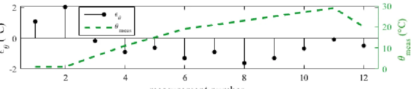
The temperature has been estimated on 12 samples corresponding to FRF measurements at 12 different temperatures between 0 and 30°𝐶and 20 modes, using Eq. (8) and the algorithm presented. The error of estimation 𝜀_𝜃 (Eq. (9)) indicates a precision of ±2°𝐶 for each path of the structure. Figure 5 shows results for path PZT 1 – PZT 2.

Figure 5 : Error of temperature estimation by MFS for 12 measurements with 20 modes.

The MFS of a mode is qualified by its coefficient of determination, so if the number of modes chosen to determine temperature is lowered, only modes with good coefficients of determination are chosen. The experiments showed that 4 modes are enough to determine the temperature, and actually, the temperature can be estimated with only 1 well-chosen mode, but other environmental parameters (or a damage) can be responsible for the frequency shift of this mode. Using several modes gives more robust temperature estimation because the estimation will be a concatenation of the temperature estimated on each mode.

Experiments were only done on one undamaged CFRP plate. Tests on other plates, with more extreme temperature, and in the presence of damage will be done to study the robustness of this method.

9 4 CONCLUSIONS AND FUTURE WORKS

The temperature has an important influence on SHM and a lot of compensation methods have been proposed in damage diagnosis. However, few studies have considered using the PZT as temperature sensors. In this article, two main axes have been developed to estimate the temperature of a CFRP plate:

 The static capacity, which is proportional to the temperature, permitted to build a database composed of the regression coefficients of the PZTs mounted on the plate. The temperature of a PZT can then be estimated with a precision of ±2°𝐶.  The modal frequency-shift (MFS) of the frequency response function obtained

with an exponential sweep signal as entry which is also proportional to temperature for most modes. It permitted to build a database with the regression coefficients of each mode for each path between PZT. The temperature of the investigated path could then be estimated with a precision of ±2°𝐶.

A combination of those two methods could allow one to determine the temperature of a structure on the PZT (static capacity method), and between PZT (MFS method). In an aeronautical context where composite structures are monitored with several PZT and subject to heterogeneous temperature variations, it could give the heat distribution of a structure without any thermometer and improve temperature compensation methods used in damage detection. A fusion of the two methods is also a way to address shortcomings from one method with the other and provide more robust results.

The presented work was realized with homogeneous temperatures on the structure under test. Complementary work is to be done to evaluate the ability of the methods described to detect local temperature variations. Experiments are also planned to check if the temperature estimation using MFS is not altered in presence of a damage.

REFERENCES

[1] G. Park, H. Sohn, C. R. Farrar, and D. J. Inman, “Overview of piezoelectric impedance-based health monitoring and path forward,” 2003.

[2] G. Park, C. R. Farrar, A. C. Rutherford, and A. N. Robertson, “Piezoelectric Active Sensor Self-Diagnostics Using Electrical Admittance Measurements,” J. Vib. Acoust., vol. 128, no. 4, p. 469, 2006.

[3] Venu Gopal Madhav Annamdas and Chee Kiong Soh, “Application of

Electromechanical Impedance Technique for Engineering Structures: Review and Future Issues,” J. Intell. Mater. Syst. Struct., vol. 21, no. 1, pp. 41–59, Jan. 2010. [4] Y. Yang, Y. Y. Lim, and C. K. Soh, “Practical issues related to the application of the

electromechanical impedance technique in the structural health monitoring of civil structures: I. Experiment,” Smart Mater. Struct., vol. 17, no. 3, p. 035008, Jun. 2008. [5] X. P. Qing, S. J. Beard, A. Kumar, K. Sullivan, R. Aguilar, M. Merchant, and M.

Taniguchi, “The performance of a piezoelectric-sensor-based SHM system under a combined cryogenic temperature and vibration environment,” Smart Mater. Struct., vol. 17, no. 5, p. 055010, Oct. 2008.

[6] B. Lin, V. Giurgiutiu, P. Pollock, B. Xu, and J. Doane, “Durability and Survivability of Piezoelectric Wafer Active Sensors on Metallic Structure,” AIAA J., vol. 48, no. 3, pp. 635–643, Mar. 2010.

[7] Y. Yang and A. Miao, “Effect of External Vibration on PZT Impedance Signature,”

Sensors, vol. 8, no. 11, pp. 6846–6859, Nov. 2008.

10

impedance-based structural health monitoring with varying temperature,” Struct. Health

Monit., vol. 10, no. 6, pp. 573–585, Nov. 2011.

[9] E. Balmes, M. Guskov, M. Rebillat, and N. Mechbal, “Effects of temperature on the impedance of piezoelectric actuators used for SHM,” 2014.

[10] B. L. Grisso and D. J. Inman, “Temperature corrected sensor diagnostics for impedance-based SHM,” J. Sound Vib., vol. 329, no. 12, pp. 2323–2336, Jun. 2010.

[11] T. G. Overly, G. Park, K. M. Farinholt, and C. R. Farrar, “Piezoelectric Active-Sensor Diagnostics and Validation Using Instantaneous Baseline Data,” IEEE Sens. J., vol. 9, no. 11, pp. 1414–1421, Nov. 2009.

[12] K.-Y. Koo, S. Park, J.-J. Lee, and C.-B. Yun, “Automated Impedance-based Structural Health Monitoring Incorporating Effective Frequency Shift for Compensating

Temperature Effects,” J. Intell. Mater. Syst. Struct., vol. 20, no. 4, pp. 367–377, Sep. 2008.

[13] D. Zhou, J. K. Kim, D. S. Ha, J. D. Quesenberry, and D. J. Inman, “A system approach for temperature dependency of impedance-based structural health monitoring” 2009, p. 72930U–72930U–10.

[14] J. Ilg, S. J. Rupitsch, and R. Lerch, “Impedance-Based Temperature Sensing With Piezoceramic Devices,” IEEE Sens. J., vol. 13, no. 6, pp. 2442–2449, Jun. 2013. [15] A. Marzani and S. Salamone, “Numerical prediction and experimental verification of

temperature effect on plate waves generated and received by piezoceramic sensors,”

Mech. Syst. Signal Process., vol. 30, pp. 204–217, Jul. 2012.

[16] O. Putkis, R. P. Dalton, and A. J. Croxford, “The influence of temperature variations on ultrasonic guided waves in anisotropic CFRP plates,” Ultrasonics, vol. 60, pp. 109–116, Jul. 2015.

[17] G. Konstantinidis, P. D. Wilcox, and B. W. Drinkwater, “An Investigation Into the Temperature Stability of a Guided Wave Structural Health Monitoring System Using Permanently Attached Sensors,” IEEE Sens. J., vol. 7, no. 5, pp. 905–912, May 2007. [18] Y. Wang, L. Qiu, L. Gao, S. Yuan, and X. Qing, “A new temperature compensation

method for guided wave-based structural health monitoring,” 2013, p. 86950H. [19] A. J. Croxford, J. Moll, P. D. Wilcox, and J. E. Michaels, “Efficient temperature

compensation strategies for guided wave structural health monitoring,” Ultrasonics, vol. 50, no. 4–5, pp. 517–528, Apr. 2010.

[20] A. J. Croxford, P. D. Wilcox, G. Konstantinidis, and B. W. Drinkwater, “Strategies for overcoming the effect of temperature on guided wave structural health monitoring,” 2007, vol. 6532, p. 65321T–65321T–10.

[21] T. Clarke, F. Simonetti, and P. Cawley, “Guided wave health monitoring of complex structures by sparse array systems: Influence of temperature changes on performance,”

J. Sound Vib., vol. 329, no. 12, pp. 2306–2322, Jun. 2010.

[22] Y. Wang, L. Gao, S. Yuan, L. Qiu, and X. Qing, “An adaptive filter-based temperature compensation technique for structural health monitoring,” J. Intell. Mater. Syst. Struct., vol. 25, no. 17, pp. 2187–2198, Nov. 2014.

[23] M. Rébillat, R. Hennequin, É. Corteel, and B. F. G. Katz, “Identification of cascade of Hammerstein models for the description of nonlinearities in vibrating devices,” J. Sound