On the importance of trip destination for modeling individual human mobility patterns

HAL Id: hal-02966791

https://hal.inrae.fr/hal-02966791

Submitted on 14 Oct 2020

HAL is a multi-disciplinary open access

archive for the deposit and dissemination of

sci-entific research documents, whether they are

pub-lished or not. The documents may come from

teaching and research institutions in France or

abroad, or from public or private research centers.

L’archive ouverte pluridisciplinaire HAL, est

destinée au dépôt et à la diffusion de documents

scientifiques de niveau recherche, publiés ou non,

émanant des établissements d’enseignement et de

recherche français ou étrangers, des laboratoires

publics ou privés.

Distributed under a Creative Commons Attribution| 4.0 International License

individual human mobility patterns

Maxime Lenormand, Juan Murillo Arias, Maxi San Miguel, José Ramasco

To cite this version:

Maxime Lenormand, Juan Murillo Arias, Maxi San Miguel, José Ramasco. On the importance of trip

destination for modeling individual human mobility patterns. Journal of the Royal Society Interface,

the Royal Society, 2020, 17 (171), pp.20200673. �10.1098/rsif.2020.0673�. �hal-02966791�

Maxime Lenormand,1 Juan Murillo Arias,2 Maxi San Miguel,3 and Jos´e J. Ramasco3

1

TETIS, Univ Montpellier, AgroParisTech, Cirad, CNRS, INRAE, Montpellier, France

2

BBVA Data & Analytics, Avenida de Burgos 16D, 28036 Madrid, Spain

3

Instituto de F´ısica Interdisciplinar y Sistemas Complejos IFISC (CSIC-UIB), Campus UIB, 07122 Palma de Mallorca, Spain

Getting insights on human mobility patterns and being able to reproduce them accurately is of the utmost importance in a wide range of applications from public health, to transport and urban planning. Still the relationship between the effort individuals will invest in a trip and its purpose importance is not taken into account in the individual mobility models that can be found in the recent literature. Here, we address this issue by introducing a model hypothesizing a relation between the importance of a trip and the distance traveled. In most practical cases, quantifying such importance is undoable. We overcome this difficulty by focusing on shopping trips (for which we have empirical data) and by taking the price of items as a proxy. Our model is able to reproduce the long-tailed distribution in travel distances empirically observed and to explain the scaling relationship between distance traveled and item value found in the data.

INTRODUCTION

Individual human mobility is a complex phe-nomenon, involving various mechanisms interacting at different spatial and temporal scales. These dynam-ics are the product of individual behaviors, governed by decisions that may depend on multiple contextual factors such as economic resources, geography, cul-ture, norms, habits or life experiences. However, be-neath this apparent complexity lies remarkable tem-poral and spatial regularities in the way people travel and interact with their environment [1]. Results ob-tained in several studies based on dollar-bill track-ing [2], mobile phone data [3], Twitter data [4, 5], Foursquare data [6] and GPS data [7] suggest that the distance ∆rbetween two consecutive locations

fol-lows an heavy-tailed distribution well approximated by a Pareto function P (∆r) ∼∆−(1+α)r with 0 < α ≤ 1.

It has also been shown that individuals tend to be at-tracted by popular places [8,9] and to return to previ-ously visited locations, thus increasing the predictabil-ity of individual human movements [10] and allowing the identification of most visited locations as well as the characterization of daily commuting patterns [11]. Individual human mobility patterns are also strongly influenced by geographical constraints [12] but also by individuals’ socio-economic status [13–15] and social network [16–19].

Based on these empirical observations, several mod-els have been proposed for modeling individual hu-man mobility patterns. The simplest type describes human traveling using L´evy Flights and Continuous Time Random Walks [2, 20]. These models give ac-curate predictions but fail at reproducing some fea-tures such as the individuals’ tendency for revisiting locations [3, 20, 21]. In [21], the authors propose a new model considering two generic mechanisms: ex-ploration and preferential return, to decide whether an individual will visit a new place or a previously vis-ited one as his/her next displacement. Going further in this direction, several models have been proposed

to take into account diverse contextual factors such as the social context, urban geography and/or type and popularity of locations [9,11,12,22].

Nonetheless, most of these models focus on sta-tionary (long-term) mobility, and, most importantly, they do not take into account the characteristics of the destination such as the travel purpose and its im-portance for the individual. Indeed, one can assume that an individual is not willing to invest the same amount of time or money, more generically, the same effort or amount of “energy” into a travel according to the value attached to the destination/objective of this travel. A basic trip purpose is the displacement between home and work, which have been collected in censuses for decades (in the US, for instance, since 1990). The introduction of new GPS-based technolo-gies have permitted to explore other trip purposes since the early 2000’s [23, 24]. Even though the re-lationship between trip cost and destination impor-tance has been postulated in transport economy, and more recently in ecology, with the use of travel cost methods to assess the value of a natural sites based on the time and travel cost expenses that people spent to visit this site [25, 26], without adequate empirical data sets to explicitly assess the “value” of a desti-nation this feature is rarely modeled at an individual scale.

The purpose of this work is to understand the displacement distribution generated by a process in which the trips have a clear purpose and, therefore, an associated objective or subjective value v. The main assumption, straightforwardly checked in the data, is that the trips’ length, d, tends to increase with v. We start by presenting a shopping mobility dataset that we use in the analysis and in which we can assign an objective meaning to v as the price of the purchased items. This dataset contains information on bank card transactions made in the provinces of Barcelona and Madrid. Inspired by search processes for wild food resources in natural environment [7,27–29], we intro-duce a human individual mobility model taking into

Number of transactions PDF 100 101 102 103 10−8 10−7 10−6 10−5 10−4 10−3 10−2 10−1 Barcelona Madrid

(a)

(b)

Figure 1. Probability density function of the number of transactions per user in 2011 (a) and the amount of money spent per transaction (b) in Barcelona (green dots) and Madrid (orange triangles).

account the value given to the trip destination through a parameter p, accounting for the probability of stop-ing or satisfystop-ing a search and that decreases when the value of v increases. The model generates trip length distributions that mimic the empirical ones and it is able to explain the observed scaling relations from the data.

MATERIAL AND METHODS Data

To explore the relationship between travel cost d and the importance given to its destination v, we analyze a credit card dataset containing information about 35 million bank card transactions made by card holders (hereafter called users) of the Banco Bil-bao Vizcaya Argentaria (BBVA) in the province of Barcelona and Madrid in 2011. Each transaction is characterized by its amount (in euro currency) and a timestamp. Each transaction is also linked to a user and a business using anonymized user and business IDs. Users are identified with an anonymized user ID and their postcode of residence. In the same way, busi-nesses are identified with an anonymized business ID, a business category (accommodation, automotive in-dustry, bars and restaurants, etc.) and the geograph-ical coordinates of the credit card terminal (see Table S2 in Supplementary Information (SI) for a full list of the selected business categories). The mobility habits and the representativeness of the BBVA credit card users in Barcelona and Madrid have already been in-vestigated in [14,30]. Here, we filtered out users with an average number of transactions per day higher than three (see the SI for more details). Only credit card payments whose amount was inferior to 500 euros have been considered. Table 1 presents the final number of users, businesses and transactions analyzed in this

study.

Table 1. Number of users, businesses and transactions in both case studies. The number of postcodes and inhabitants and the surface area of the two provinces are also displayed.

Statistics Barcelona Madrid Number of postcodes 364 268 Number of inhabitants 5,540,925 6,489,680 Area (km2_{) 7,733 8,022} Number of users 269,849 528,719 Number of businesses 111,267 108,936 Number of transactions 12,993,179 24,507,586

The probability density function (PDF) of the num-ber of transactions per user in 2011 and the amount of money spent per transaction is displayed in Figure

1. We observe a strong heterogeneity among users re-garding the number of transactions. The median value is 27 and the lower quartile is 8 in both provinces, the upper quartile is 69 for Barcelona and 66 for Madrid. Between 10 and 70 euros are spent in 50% of the actions with a median amount of 30 euros per trans-action.

For each transaction, the cost d associated to a travel is estimated with the distance between the user’s postcode of residence (lon/lat coordinates of the centroid) and the location of the business in which the transaction occurred (lon/lat of the credit card termi-nal). The value v given to the travel purpose is in-ferred by the amount of money spent per transaction. The amount of money spent v is divided into five inter-vals (]0, 50[, [50, 75[, [75, 100[, [100, 200[, [200, 500[).

time t

time t+1

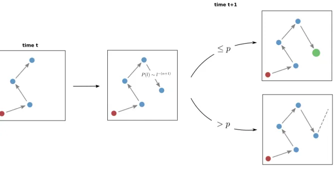
Figure 2. A schematic diagram of the model. At each step, the individual leaves his/her actual location and moves in a random direction at a distance sample from a Pareto distribution P (l) = αl0α

lα+1. If the new location falls outside of the square

boundaries the sampling process is repeated. According to the value v given to the trip destination, the individual will then decide to stop or not his/her journey with a probability p. If the individual decides to end his/her journey the final destination is drawn at random in a circle of radius r around the last position (green circle).

Model

The proposed model can be interpreted as a search process that stops when a satisfying object (destina-tion) has been found [31]. The rules of the model are outlined in Figure2 . We assume that an individual starts the travel at his/her actual location (at home or work, for instance). The position of this first lo-cation is drawn at random in a square of lateral size L expressed in kilometer. In practice, this param-eter allows to take into consideration the geograph-ical constraints of a case study site (administrative or geological boundaries for example). At each step, the individual move in a random direction and at a random distance sampled from a Pareto distribution P (l) = α l0

α

l−α−1, where α is the exponent and l0

the minimum spatial scale considered. At each step, the possibility to end the travel is represented by a probability p of fulfilling the trip goal. Note that un-like most of the models described in the introduction, since only short-range mobility patterns are consid-ered, our model does not take explicitly into account time. The probability of stopping p is assumed to have an inverse relation with the importance given to the trip goal v. The higher the value v associated to the objective of the travel, the longer the search process (i.e., low value of p) and the higher the dis-tance d between origin and destination can become. If the purpose of the trip is a search to buy an ob-ject, the individuals would be willing to explore more shops or to travel further as the item price increases (buying a car requires more “energy” than a piece of

bread). Finally, when the individual decides to end his/her journey the final destination is drawn at ran-dom in a circle of radius r around the last position. This mechanism is included to take into account the uncertainty present in the data on the exact position of the retailing center. Still, in case of a more abstract framework the model could be simplified by making r → 0 and setting the purchase place in the current agent’s location.

Model calibration

The comparison between model and data is based on the probability density function (PDF) of the dis-tance d between the origin and the destination. The simulated PDF is obtained with 100,000 simulations of the model. The model has five parameters L, α, l0, r and p. L controls the size of the modeling area,

l0 and r the minimum spatial resolution, α the jump

length and p the users’ tendency to explore the mod-eling area. The free parameter l0and r allows notably

to control the users’ exploration behavior at short dis-tance from home. The numerical values of these five parameters were determined from the empirical data in two steps and independently for both provinces. We first adjusted the five parameters’ value by minimizing the Kolmogorov-Smirnov distance between observed and simulated PDF of d (all values of v combined). We then adjusted the value of p according to the PDF of d for each interval of amount of money spend v.

d (km)

PDF

d d

PDF

(d)

d (km)

PDF

(c)

d d

PDF

(b)

(a)

(c)

Figure 3. Probability density function of the distance d from the residence and the final location as a function of p obtained with the calibrated model for Barcelona. The original distributions are shown in (a) and (c), while the normalized distributions obtained by dividing by the median distance ¯d are in (b) and (e). In (a) and (b), there is no bounding box, L = ∞, while in (c) and (d) L = 100 km.

Model features

Every agent in the model is performing a short L´evy flight in the limited space provided by the box of side L. To better understand the model features, it is help-ful to to take first the limits L → ∞, so there is no spatial constraint. The L´evy flight is not, actually, complete because we introduce a stopping mechanism with p. It implies that the number of jumps, n, that an agent takes follows the geometric distribution:

Pn(n) = (1 − p)n−1p. (1)

The average number of jumps is thus given by ⟨n⟩ = 1/p. Lower p means more jumps and, therefore, the potential for longer distances in the distribution of dis-tance from the origin to the purchase location, P (d). Recalling that p will be related to v with an inverse function, larger v implies as well longer distances d. The distribution P (d) comes thus from the

aggrega-tion of a finite number n of L´evy jumps. In the limit n → ∞, it could be expressed in function of the L´evy α-stable distributions. On the contrary, for small n the analytical expression of P (d) does not correspond to L´evy’s generalization of the central limit theorem. In any case, there is an inverse relation between the median of the distance d, ¯d, and p. Examples of the distributions P (d) for different values of p can be seen in Figure3(a). The range of small d values is flattened by the presence of a minimal scale (controlled by l0

and r), whereas as expected a long power-law like tail appears for large d. In this case, there is no other characteristic scales in the model beyond the small scale and ¯d as shown by the collapse of the curves for different p obtained dividing the x-axis by ¯d and normalizing the distributions again (Figure3(b)).

The picture changes if L and, consequently, the bounding box is finite. The limited L´evy flights are then occurring inside a constrained space and those

v< 50 v∈[50,75[ v∈[75,100[ v∈[100,200[ v∈[200,500[

d (km)

PDF

(a)

d (km)

PDF

(b)

Figure 4. Distribution of the distance traveled according to the amount of money spent in Barcelona (a) and Madrid (b). Probability density function of the distance between the users’ place of residence and the location of the business in which the transaction occurred according to the amount of money spent v. The color of the curves represents different ranges of amount of money spent.

jumping outside are not considered. This introduces a maximum scale in the P (d) distributions as can be seen in Figure 3(c), which manifests in a fast (exponential-like) decay for large values of d. The curves still maintained the power law-like properties and the possibility of collapse dividing d by ¯d, but in a restricted domain of d values (see Figure3(d)).

RESULTS

We start by exploring empirically the relationship between the travel distance d and the importance given to its destination v. Figure4displays the prob-ability density function of the distance between the users’ home and the location of the business in which the transaction occurred according to the amount of money spent v divided into five intervals. Several regimes can be observed. First, the probability to travel a certain distance to make a purchase increases, reaching a maximum between 500 m and 1 km, and, then, the probability starts to decrease, slowly at first, and then more rapidly, exhibiting a power-law like de-cay. Finally, after 20 − 50 km the province boundaries act as a natural cutoff in the distribution (our data is limited to single provinces). The shape of distribu-tion is very similar for each range of amount of money spent. It seems however that the distance traveled globally increases with the amount of money spent.

Figure5a shows for each range of values v the me-dian distance traveled ¯d as a function of the median amount of money spent ¯v. Although the distance trav-eled is globally higher in Madrid than in Barcelona, the distance traveled increases with the amount of money spent following the scaling relationship ¯d ∼ ¯vγ in both provinces. We obtain a value γ = 0.23 ± 0.02

for Barcelona and γ = 0.15±0.03 for Madrid estimated with a log-log regression. It is interesting to note that this relation between d and v seems to be the unique driver of the differences observed between the PDFs in Figure 4. Reminding the collapse in the model in Figure3, as can be seen in Figure5b a scaling factor depending only on ¯d can be used to visually collapse all the PDFs shown in Figure 5b into a single curve (except for the maximum values constrained by the provinces’ geographical boundaries). This suggests that the mechanisms underlying trip generation are the same for all price ranges and the only difference is a characteristic distance ¯d, which is a function of the price v of the item to purchase.

Nevertheless, we need to verify that this result holds whenever the spatial distributions and types of users and businesses. To ensure that it is the case, we plot in Figure 6 the distribution of the exponent γ esti-mated with a log-log model for each postcode in both provinces. The value of γ is globally strictly higher than 0, suggesting that the positive correlation be-tween ¯d and ¯v does not dependent of the user’s post-code of residence. Moreover, this positive correlation between the two quantities is independent of the users’ sociodemographic characteristics (gender, age and oc-cupation) and the business categories (see the SI for more details).

We now focus on the results obtained with our model in order to reproduce and explain the relation-ship between d and v observed in the data. As de-scribed in Material and Methods, we first consider the distribution of all the amounts combined in order to calibrate the five parameters. As it can be seen in Fig-ure7, the fit is quite good. We obtain similar results in both provinces. The modeling area represented by a square of lateral size L is bigger in Barcelona (100

2.0 2.5 3.0 3.5 4.0 4.5 5.0 5.5 101 102

v (in euro)

d

(in km)

(a)

d d

PDF

(b)

Figure 5. Scaling relationship between amount of money spent and distance traveled. (a) Median distance ¯d as a function of the median amount of money spent ¯v for each range of prices in Barcelona (green dots) and Madrid (orange triangles). (b) Probability density function of the distance normalized by the median distance according to the amount of money spent v in Barcelona (solid line) and Madrid (dashed line). The color of the curves represents different ranges of amount of money spent. 0.0 0.5 1.0 1.5 0 1 2 3 4 γ PDF Barcelona Madrid

Figure 6. Probability density function of the exponent γγγ estimated with a log-log model for each postcode in the provinces of Barcelona and Madrid.

km) than in Madrid (75 km). The parameter α, expo-nent of the Pareto distribution, is equal to 0.6 which is consistent with values obtained in other studies [2–7]. We obtain a value of p equal to 0.3 in Barcelona and 0.25 in Madrid, this value, comprised between 0 and 1, has an inverse relation to the energy that people are willing to invest in order to go shopping in both provinces.

Finally, we explore the behavior of p according to the median amount of money spent ¯v. The results obtained are plotted in Figure 8a. As expected, the value of p decreases with increasing v, which implies that the distance traveled grows with the price of the item to purchase. Furthermore, we find that a scaling

relation of the type p ∼ ¯v−β adjusts well to the data. We obtain a value β = 0.24 ± 0.01 for Barcelona and β = 0.14 ± 0.02 for Madrid estimated with a log-log re-gression. However, keep in mind that the model does not impose a given relation between p and ¯v, it can be general with different type of data leading to diverse relationships (or exponents if the power-law scaling holds). In our case, both ¯d and p can be expressed as scaling functions of ¯v. It is, therefore, important to understand the relation between the direct observ-able in mobility ¯d and our model’s p. If the basic displacement distribution had had a finite second mo-ment, i.e., the movement was a random walk in 2D, it would have been possible to find analytical approx-imations for the final distance. However, this task becomes complex with a finite number of steps in a L´evy flight.

Therefore, to analyze the relationship between γ and β, we assume a relation p ∼ ¯v−β to generate five p values for a given β value. We normalize the five p values in order to preserve the average value ob-served in the data (i.e. values displayed in Figure8a). We then simulate the five ¯d value associated with the p values with our model (using the calibrated L, α, l0 and r values for both provinces). We finally

esti-mate the exponent γ from ¯d ∼ ¯vγ _{and compare the}

values of γ obtained versus those of the corresponding β. The results of this exercise are shown in Figure

8b. The relation is linear and close to the identity (∼ 0.9) but we note a slight difference between the re-sults obtained with the model parameterization used for Barcelona and Madrid. This is mainly due to the size of modeling area L. The grey dashed line in Fig-ure 8b represents the relationship between γ and β obtained with an infinite modeling area. The effect

d (km)

PDF

(a)

d (km)

PDF

(b)

Figure 7. Comparison between data and model. Probability density function of the distance between the users’ place of residence and the location of the business in which the transaction occurred (all of the amounts combined) obtained with the data (in blue) and the calibrated model (in red). (a) In Barcelona the best results are obtained with a square of side length L = 100 km, a radius r equal to 300 meters, mobility parameters l0=300 meters, α = 0.6 and p = 0.3. (b) In Madrid the best results are obtained with a square of side length L = 75 km, a radius r equal to 400 meters, mobility parameters l0=400 meters, α = 0.6 and p = 0.25.

of increasing the value of L on the slope of the linear relationship is also exposed in Figure 8c. We observe that the slope ranges from 0.85 to 1.1 for value of L lower than 500 km, after that it increases slowly until reaching the asymptotic value 1.33. This change in the slope is essentially due to the progressive reduction of the sum of L´evy flights’ truncation. It is worth noting that the slope obtained with values of L reflecting an intra-urban mobility scale are very closed to one. An equality between γ and β is also consistent with the empirical observations made in Barcelona and Madrid (Figure 8b), suggesting that the probability to stop the journey could be inversely proportional to the me-dian distance traveled (p ∼ 1/ ¯d).

DISCUSSION

In summary, we introduced a model of individual human mobility patterns able to reproduce and ex-plain the relationship between the travel cost associ-ated to a trip and the importance given to its des-tination observed in credit card data recorded in the provinces of Barcelona and Madrid in 2011. In partic-ular, we have shown that the distances between place of residence and place of purchase increase with the amount of money spent following a similar scaling re-lationship in both provinces. The model that we pro-posed is able to reproduce these behaviors and also to mimic the final scaling relation.

Overall, we observed a good agreement between the results obtained in Barcelona and Madrid. Both provinces show similar trends in the relationship be-tween amount of money spent and distance traveled.

The exponent values observed in the scaling relation-ships are of the same order of magnitude in both provinces and the calibrated parameter values ob-tained with the model are also very similar. More research is needed to elucidate whether the patterns found are common to other countries and cities, and, specially, whether the small differences are related to the diverse city shapes or the geographical structure of the administrative units.

Limitations of the study

The results obtained give a good confidence in the robustness of the scaling relationship observed in the data by assessing the effect of the users’ character-istics and business category on the exponent of the scaling relationship in the two provinces. However, it will be important to evaluate our hypothesis and our model on case studies coming from other coun-tries/continents and on different data sources. A lim-itation of the study lies in the nature of our data sam-ples spatially constrained by the province boundaries. This forces us to include in the model a bounding box and restricts our capability to reach analytical re-sults. As in [30], we also assumed that every shopping trip starts at home and ends at the place of purchase without considering more complicated case including sequences of purchases. Nevertheless, we replicated the analysis considering, for each user, only days with a unique transaction and we obtained very similar re-sults (see Figure S3 in SI). Finally, online shopping could be also a handicap for our analysis. Unfortu-nately, we cannot distinguish online and offline shops

0.15 0.20 0.25 0.30 0.35 0.40 101 102 v (in euro) p Barcelona Madrid (a) 0.0 0.2 0.4 0.6 0.8 1.0 0.0 0.2 0.4 0.6 0.8 1.0 β γ (b) Model (L=∞) Model (L=100) Model (L=75) Barcelona Madrid 0 500 1000 1500 0.8 0.9 1.0 1.1 1.2 1.3 1.4 L Slope (c) Barcelona Madrid

Figure 8. Relationship between γγγ and βββ. (a) Probability p as a function of the amount of money spent v in each bin in Barcelona (green dots) and Madrid (orange triangles). (b) Relation between γ and β obtained with the model and the data for Barcelona (in green) and Madrid (in orange). The lines correspond to the simulations and the symbol to the data (Barcelona in green and Madrid in orange). The grey solid line corresponds to the results obtained with the model with L = ∞. (c) Evolution of the slope between γ and β as a function of L for Barcelona (green dots) and Madrid (orange triangles).

in our data. Online shopping has become more rele-vant with time, its presence was not so strong in the shopping mixing of 2011 as today, and the retailer must be included in the same province is a strict lim-itation for most of the online shops. In the online purchases, the distance should not be anymore an im-portant variable and it should not show a clear rela-tion with v, given that it is possible to buy equally items of any price.

Concluding Remarks

To conclude, this study is a first attempt to quan-tify the relationship between travel cost associated to a trip and importance given to its destination. The results obtained in this study shed new light on the modeling of human mobility patterns at an individ-ual scale. We are quite aware that trip motivations are very complicated to quantify but we truly believe that it is an important topic. An accurate modeling of daily human mobility patterns in cites is crucial in

a wide range of applications. Getting better insights on the relationship between trip characteristics and travel motivations would allow to gain a better un-derstanding of urban dynamics in order to optimize cities. We hope that more and more (hopefully open) data will be made available in years to come to study the importance of trip destination and its role in the modeling of human mobility patterns.

ACKNOWLEDGEMENTS

ML thanks the French National Research Agency for its financial support (project NetCost, ANR-17-CE03-0003 grant). MSM and JJR acknowledge par-tial funding from the Spanish Ministry of Science, In-novation and Universities, the National Agency for Research Funding AEI and FEDER (EU) under the grant PACSS (RTI2018-093732-B-C22) and the Maria de Maeztu program for Units of Excellence in R&D (MDM-2017-0711). We also thank Teodoro Danne-mann for fruitful discussions.

[1] H. Barbosa, M. Barthelemy, G. Ghoshal, C. R. James, M. Lenormand, T. Louail, R. Menezes, J. J. Ramasco, F. Simini, and M. Tomasini. Human mobility: Models and applications. Physics Reports, 734:1–74, 2018. [2] D. Brockmann, L. Hufnagel, and T. Geisel. The

scal-ing laws of human travel. Nature, 439(7075):462–465, 2006.

[3] M. C. Gonz´alez, C. A. Hidalgo, and A.-L. Barab´asi. Understanding individual human mobility patterns. Nature, 453(7196):779–782, 2008.

[4] B. Hawelka, I. Sitko, E. Beinat, S. Sobolevsky, P. Kazakopoulos, and C. Ratti. Geo-located twitter as a proxy for global mobility patterns. Cartography and Geographic Information Science, 41:260–271, 2014.

[5] M. Lenormand, B. Goncalves, A. Tugores, and J. J. Ramasco. Human diffusion and city influence. Journal of Royal Society Interface, 12:20150473, 2015. [6] Z. Cheng, J. Caverlee, K. Lee, and D. Sui. Exploring

millions of footprints in location sharing services. Pro-ceedings of the Fifth International AAAI Conference on Weblogs and Social Media, 2011.

[7] D. A. Raichlen, B. M. Wood, A. D. Gordon, A. Z. P. Mabulla, F. W. Marlowe, and H. Pontzer. Evidence of L´evy walk foraging patterns in human hunter-gatherers. Proceedings of the National Academy of Sciences, 111(2):728–733, 2014.

[8] C. Roth, S. M. Kang, M. Batty, and M. Barthelemy. Structure of Urban Movements: Polycentric Activ-ity and Entangled Hierarchical Flows. PLoS ONE,

6(1):e15923, 2011.

[9] S. Hasan, C. M. Schneider, S. V. Ukkusuri, and M. C. Gonz´alez. Spatiotemporal patterns of urban human mobility. Journal of Statistical Physics, 151(1-2):304– 318, 2013.

[10] C. Song, Z. Qu, N. Blumm, and A.-L. Barab´asi. Lim-its of Predictability in Human Mobility. Science, 327(5968):1018–1021, 2010.

[11] C. M. Schneider, V. Belik, T. Couronn´e, Z. Smoreda, and M. C. Gonz´alez. Unravelling daily human mo-bility motifs. Journal of The Royal Society Interface, 10(84):20130246, 2013.

[12] C. Kang, X. Ma, D. Tong, and Y. Liu. Intra-urban human mobility patterns: An urban morphology per-spective. Physica A: Statistical Mechanics and its Ap-plications, 391(4):1702–1717, 2012.

[13] L. Lotero, A. Cardillo, R. Hurtado, and J. Gomez-Gardenes. Several multiplexes in the same city: The role of socioeconomic differences in urban mobility. Available at SSRN 2507816, 2014.

[14] M. Lenormand, T. Louail, O. Garcia Cant´u, M. Pi-cornell, R. Herranz, M. Barthelemy, M. San Miguel, and J. J. Ramasco. Influence of sociodemographic characteristics on human mobility. Scientific Reports, 5:10075, 2015.

[15] L. Gauvin, M. Tizzoni, S. Piaggesi, A. Young, N. Adler, S. Verhulst, L. Ferres, and C. Cattuto. Gen-der gaps in urban mobility.https://arxiv.org/abs/

1906.09092, 2019.

[16] D. Wang, D. Pedreschi, C. Song, F. Giannotti, and A.-L. Barab´asi. Human mobility, social ties, and link pre-diction. In Proceedings of the 17th ACM SIGKDD In-ternational Conference on Knowledge Discovery and Data Mining, KDD ’11, pages 1100–1108, 2011. [17] P. A Grabowicz, J. J. Ramasco, B. Gon¸calves, and

V. M Egu´ıluz. Entangling mobility and interactions in social media. PLoS ONE, 9:e92196, 2014.

[18] M. Picornell, T. Ruiz, M. Lenormand, J. J. Ramasco, T. Dubernet, and E. Fr´ıas-Mart´ınez. Exploring the potential of phone call data to characterize the rela-tionship between social network and travel behavior. Transportation, 42(4):647–668, 2015.

[19] J. L. Toole, C. Herrera-Yaq¨ue, C. M. Schneider, and M. C. Gonz´alez. Coupling human mobility and so-cial ties. Journal of The Royal Society Interface, 12(105):20141128, 2015.

[20] I. Rhee, M. Shin, S. Hong, K. Lee, and S. Chong. On the levy-walk nature of human mobility. In

INFO-COM 2008. The 27th Conference on Computer Com-munications. IEEE, 2008.

[21] C. Song, T. Koren, P. Wang, and A.-L. Barab´asi. Modelling the scaling properties of human mobility. Nature Physics, 6(10):818–823, 2010.

[22] K. Lee, S. Hong, S. J. Kim, I. Rhee, and S. Chong. SLAW: A Mobility Model for Human Walks. In Pro-ceedings of the 28th Annual Joint Conference of the IEEE Computer and Communications Societies (IN-FOCOM), 2009.

[23] J. Wolf, R. Guensler, and W. Bachman. Elimina-tion of the travel diary: Experiment to derive trip purpose from global positioning system travel data. Transportation Research Record, 1768:125–134, 2001. [24] W. Bohte and K. Maat. Deriving and validating trip purposes and travel modes for multi-day gps-based travel surveys: A large-scale application in the nether-lands. Transportation Research Part C: Emerging Technologies, 17:285–297, 2009.

[25] G. R. Parsons. The Travel Cost Model. In P. A. Champ, K. J. Boyle, and T.s C. Brown, editors, A Primer on Nonmarket Valuation, The Economics of Non-Market Goods and Resources. Springer Nether-lands, Dordrecht, 2003.

[26] B. J. Butterfield, A. L. Camhi, R. L. Rubin, and C. R. Schwalm. Chapter Five - Tradeoffs and Compatibil-ities Among Ecosystem Services: Biological, Physi-cal and Economic Drivers of Multifunctionality. In G. Woodward and D. A. Bohan, editors, Advances in Ecological Research, volume 54 of Ecosystem Services: From Biodiversity to Society, Part 2, pages 207–243. Academic Press, 2016.

[27] G. M. Viswanathan, V. Afanasyev, S. V. Buldyrev, E. J. Murphy, P. A. Prince, and H. E. Stanley. L´evy flight search patterns of wandering albatrosses. Na-ture, 381(6581):413–415, 1996.

[28] G. M. Viswanathan, S. V. Buldyrev, S. Havlin, M. G. E. da Luz, E. P. Raposo, and H. E. Stanley. Optimizing the success of random searches. Nature, 411:911–914, 1999.

[29] G. M. Viswanathan. Ecology: Fish in L´evy-flight for-aging. Nature, 465(7301):1018–1019, 2010.

[30] T. Louail, M. Lenormand, J. M. Arias, and J. J. Ram-asco. Crowdsourcing the Robin Hood effect in cities. Applied Network Science, 2(1):11, 2017.

[31] G. Carra, I. Mulalic, M. Fosgerau, and M. Barthelemy. Modelling the relation between income and commuting distance. Journal of The Royal Society Interface, 13(119):20160306, 2016.

APPENDIX Data preprocessing

As mentioned in the main text, we analyzed in this study a credit card dataset containing information about 35 million bank card transactions made by credit card users of the Banco Bilbao Vizcaya Argentaria (BBVA) in the province of Barcelona and Madrid in 2011. The dataset used in this study has been already presented and analyzed in [14]. We only applied two filters, one on the average number of transactions per day and another one on the maximum amount of money spent per transaction.

First, we filtered out users with a number of transactions per day higher than three. We determined this threshold by plotting the number of transactions per user as a function of the number of days with at least one transaction. We observe in Figure S1 that most of the users made less than three transactions per day (red line). Only a few users (234 for Barcelona and 613 for Madrid) made more than three transactions per day in 2011 representing less than 0.12% of the users in both case studies.

Figure S1. Number of transactions as a function of the number of days with at least one transaction in 2011 in Barcelona (a) and Madrid (b). Each blue dot represents a user. The red line represents the threshold of three transactions per day.

Then we removed from the database all the transaction with an amount higher than 500 euros (85,665 for Barcelona and 183,155 for Madrid) representing less than 0.75% of the transactions in both case studies.

Effect of the users’ characteristics on the exponent γ

As mentioned in the main text the relationship between the median distance ¯d and the median amount of money spent ¯v can be well-approximated by a log-log function. However, we need to verify that this positive correlation between the two quantities does not depend of the users’ sociodemographic characteristics. Each BBVA user is connected with sociodemographic characteristics (gender, age and occupation). For the sake of convenience, we consider five age groups (]15, 30], ]30, 45], ]45, 60], ]60, 75], > 75) and five types of occupations (student, unemployed, employed, homemaker, and retired). The relationship between the distance traveled ¯d and the amount of money spent v according to the users’ sociodemographic characteristics is displayed in Table S1. Here again, the value of γ is always strictly higher than 0.

Effect of business category on the exponent γ

Finally, we need to verify that the positive correlation between the median distance ¯d and the amount of money spent v does not depend on the type of purchases (i.e. business category) in the two provinces. The different business categories and their proportions of associated transactions are available in Table S2. The relationship between the distance traveled and the amount of money spent according to the business category is presented in Table S3. In most of the cases, the value of γ is strictly higher than 0. Note that in some cases, like for the Restaurants business category for example, due to the presence of outlier (Figure S2) no log-log relationship between ¯d and v has been found.

Table S1. Relationship between the distance traveled and the amount of money spent according to the users’ economic and sociodemographic characteristics.

Category Median Distance (BCN / MAD) Slope (BCN / MAD) R2 (BCN / MAD) Total 2.41 / 3.49 0.23 / 0.15 0.97 / 0.91 Men 2.98 / 3.97 0.2 / 0.15 0.99 / 0.87 Women 2.11 / 3.11 0.2 / 0.13 0.93 / 0.84 Age ∈ ]15,30] 3.14 / 4.65 0.17 / 0.13 0.99 / 0.91 Age ∈ ]30,45] 2.52 / 3.92 0.26 / 0.18 0.98 / 0.86 Age ∈ ]45,60] 2.15 / 2.75 0.26 / 0.24 0.96 / 0.96 Age ∈ ]60,75] 1.84 / 2.21 0.28 / 0.27 0.99 / 0.99 Age > 75 1.43 / 1.59 0.26 / 0.22 0.92 / 0.99 Student 3.13 / 4.49 0.08 / 0.08 0.92 / 0.87 Unemployed 2.12 / 3.1 0.25 / 0.18 0.95 / 0.95 Employed 2.54 / 3.77 0.23 / 0.15 0.97 / 0.85 Homemaker 1.79 / 2.31 0.25 / 0.2 0.97 / 0.89 Retired 1.69 / 2.02 0.23 / 0.23 0.97 / 0.99

Table S2. Percentage of transaction associated to each of the 20 business categories selected.

Category Barcelona Madrid

Supermarket 18.13 16.1

Hypermarket 9.24 11.75

Gas Stations 12.18 11.06

Clothing store chain 4.35 7.23

Restaurants 8.38 6.59

Department store 2.12 5.08 Clothing store chain 5.54 4.58 Pharmacy, optical and orthopedics 4.23 3.78

Retail store 6.32 2.97

Hair and beauty 2.76 2.63 Fast food restaurants and chains 1.02 2.28

Bars and cafe 1.78 1.56

Shoe store 1.57 1.38

Toys and sports articles 1.52 1.37 Electronics, computers and appliances 1.49 1.35 Car dealership, garage and spare parts distributors 1.18 1.1

Bazaar 0.99 1.08

Bookshop, music shop and stationery 1.32 1.02

DIY store 0.75 0.95

Table S3. Relationship between the distance traveled and the amount of money spent according to the business category.

Category Median Distance (BCN / MAD) Slope (BCN / MAD) R2 (BCN / MAD) Supermarket 1.38 / 1.83 0.4 / 0.13 0.85 / 0.98 Hypermarket 2.08 / 2.4 0.37 / 0.25 0.91 / 0.93 Gas Stations 3.22 / 3.71 0.48 / 0.54 0.93 / 0.91 Clothing store chain 4.42 / 4.94 0.02 / -0.01 0.13 / 0.48 Restaurants 5.01 / 5.52 0.03 / -0.04 0.1 / 0.21 Department store 3.68 / 4.82 0.02 / -0.03 0.8 / 0.34 Clothing store chain 2.56 / 4.06 0.14 / 0.07 0.98 / 0.88 Pharmacy 1.52 / 2.01 0.15 / 0.02 0.89 / 0.27 Retail store 1.46 / 1.86 0.24 / 0.18 0.93 / 0.69 Hair and beauty 1.65 / 2.04 0.18 / 0.19 0.89 / 0.92 Fast food restaurants 4.94 / 5.31 -0.15 / -0.11 0.92 / 0.97 Bars and cafe 4.26 / 4.99 -0.07 / -0.11 0.34 / 0.89 Shoe store 2.21 / 3.36 0.21 / 0.12 0.98 / 0.92 Toys and sports articles 3.27 / 5.4 0.24 / 0.09 0.91 / 0.9 Electronics 4.56 / 5.96 0.07 / 0.1 0.93 / 0.89 Car dealership 3.35 / 4.64 -0.08 / -0.04 0.77 / 0.85 Bazaar 2.45 / 3.42 0.22 / 0.1 0.96 / 0.99 Bookshop 2.47 / 3.65 0.07 / -0.14 0.91 / 0.71 DIY store 5.3 / 8.93 0.15 / 0.1 0.98 / 0.92 Hospitals 2.62 / 3.5 0.08 / 0.06 0.9 / 0.45

4.0

4.5

5.0

5.5

6.0

10

10

v (euro)

d

Supplementary Figures

2

3

4

5

6

10

10

v (in euro)

d

(in km)

Barcelona

Madrid

Figure S3. Scaling relationship between amount of money spent and distance traveled based on daily-unique transac-tion. Median distance ¯d as a function of the median amount of money spent ¯v for each range of prices in Barcelona (green dots) and Madrid (orange triangles). We define a daily-unique transaction as a transaction made by a user during a day where she or he made only one transaction. They represent 39.77% of the transaction in Barcelona and 40.07% in Madrid.