optimization in multicriteria problems
Lucie Galand, Patrice Perny, and Olivier Spanjaard
LIP6-UPMC, 104 av. du Pr´esident Kennedy 75016 Paris, France [email protected]
Summary. This paper is devoted to the search for Choquet-optimal solutions in multicriteria combinatorial optimization with application to spanning tree problems and knapsack problems. After recalling basic notions concerning the use of Cho-quet integrals for preference aggregation, we present a condition (named preference for interior points) that characterizes preferences favouring well-balanced solutions, a natural attitude in multicriteria optimization. When using a Choquet integral as preference model, this condition amounts to choosing a submodular (resp. super-modular) capacity when criteria have to be minimized (resp. maximized). Under this assumption, we investigate the determination of Choquet-optimal solutions in the multicriteria spanning tree problem and the multicriteria 0-1 knapsack problem. For both problems, we introduce a linear bound for the Choquet integral, computable in polynomial time, and propose a branch and bound procedure using this bound. We provide numerical experiments that show the actual efficiency of the algorithms on various instances of different sizes.
Key words: Multicriteria combinatorial optimization, Choquet integral, branch and bound, minimal spanning tree problem, knapsack problem.
1 Introduction
In combinatorial multicriteria optimization problems, many fruitful studies concern the determination or the approximation of the Pareto set (Ehrgott, 2005). However, in some applications, the size of the instances as well as the combinatorial nature of the space of feasible solutions make it impossible to generate the whole set of Pareto solutions (the number of Pareto solutions grows, in the worst case, exponentially with the size of the instance (Hamacher and Ruhe, 1994) and the number of criteria (Rosinger, 1991)). Moreover many solutions in the Pareto set are not relevant for the decision maker because they do not match his expectations on some criteria. When a model of decision maker’s preferences is available, it is worth trying to focus the search directly on the most preferred solutions, rather than generating the entire Pareto set (Galand and Spanjaard, 2007; Galand and Perny, 2007; Perny et al., 2007). Among the various preference models considered in the literature on
multicriteria decision making, the Choquet integral is certainly one of the most expressive aggregators (see Grabisch et al. (2000)). This model makes it possible to take into account the interactions between criteria and to direct the search towards the desired compromise solution. Moreover, it is able to reach supported as well as unsupported solutions within the Pareto set.
For this reason, we assume in this work that the preferences of the decision maker are known and represented by a Choquet integral. More precisely, to restrict the search on well-balanced solutions we only consider the subfamily of Choquet integral operators with a capacity of a specific shape, namely a submodular capacity when criteria have to be minimized and a supermodular one when they have to be maximized (see Chateauneuf and Tallon (2002)). Then we investigate the search for Choquet-optimal solutions in the multicriteria spanning tree problem (the single criterion version of which is polynomial) and the multicriteria 0-1 knapsack problem (the single criterion version of which is NP-hard).
The paper is organized as follows. In Section 2, we recall basic features of Cho-quet integral operators. Then we formulate a condition characterizing preferences favouring well-balanced solutions and show how it leads to adopt a submodular (resp. supermodular) capacity when criteria have to be minimized (resp. maximized). In Section 3, we propose a branch and bound procedure based on an efficiently com-putable bound on the value of a Choquet-optimal solution. In Section 4, we report numerical experiments showing the efficiency of the proposed algorithms.
2 Choquet integral and well-balanced solutions
We consider alternatives that are valued according to multiple criteria functions ci,
i ∈ Q = {1, . . . , q}. Without loss of generality, we assume here that the perfor-mances on criteria functions are integer. Every alternative is therefore characterized by a vector of performances in Nq. A popular approach to compare vectors of
per-formance is to use an aggregation function that associates each alternative with a single scalar value. The Choquet integral (Choquet, 1953) is an aggregation function that generalizes the notion of average when weights are represented by a capacity. Definition 1 A capacity is a set function v : 2Q→ [0, 1] such that:
• v(∅) = 0, v(Q) = 1 • ∀A, B ∈ 2Q
such that A ⊆ B, v(A) ≤ v(B)
For any subset A ⊆ Q, v(A) represents the importance of coalition A. Let us now recall some definitions about capacities.
Definition 2 A capacity v is said to be supermodular when v(A ∪ B) + v(A ∩ B) ≥ v(A) + v(B) for all A, B ⊆ Q, and submodular when v(A ∪ B) + v(A ∩ B) ≤ v(A) + v(B) for all A, B ⊆ Q. A capacity v is said to be additive when it is supermodular and submodular simultaneously.
Note that when v is additive, it is completely characterized by vi = v({i}), i =
1, . . . , q since v(A) =P
Definition 3 To any capacity v, we can associate a dual capacity ¯v defined by ¯
v(A) = 1 − v(Q \ A) for all A ⊆ Q. Obviously, ¯¯v = v for any capacity v.
It is well known that ¯v is submodular if and only if v is supermodular and vice-versa. Note that when v is supermodular, we have v(A) + v(Q \ A) ≤ 1, hence v(A) ≤ ¯v(A). In this case, Shapley (1971) has shown that v has a non-empty core, the core being defined by:
core(v) = {λ ∈ L : v(A) ≤ λ(A) ≤ ¯v(A)}
where L is the set of additive capacities. Similarly, when v is submodular, then core(¯v) = {λ ∈ L : ¯v(A) ≤ λ(A) ≤ v(A)} is non-emtpy since ¯v is supermodular. These results will be used in Section 3.
The Choquet integral of a vector x ∈ Nq with respect to a capacity v is defined by:
Cv(x) = q
X
i=1
ˆv(X(i)) − v(X(i+1))˜ x(i) (1)
=
q
X
i=1
ˆx(i)− x(i−1)˜ v(X(i)) (2)
where (.) represents a permutation on {1, . . . , q} such that 0 = x(0)≤ x(1)≤ . . . ≤
x(q), X(i) = {j ∈ Q, xj ≥ x(i)} = {(i),(i + 1), . . ., (q)} for i ≤ q and X(q+1) = ∅.
Note that X(i+1) ⊆ X(i), hence v(X(i)) ≥ v(X(i+1)) for all i. The Choquet integral
generalizes the classical notion of average with the following interpretation based on Equation (2): for a given vector x = (x1, . . . , xq), the performance is greater or equal
to x(1) on all criteria belonging to X(1), which represents a weight of v(X(1)) = 1,
then the performance is greater or equal to x(2) on all criteria belonging to X(2),
which represents an increment of x(2)−x(1)with weight v(X(2)). A similar increment
applies from x(2) to x(3) with weight v(X(3)), and so on. The overall integral is
therefore obtained by aggregation of marginal increments x(i)− x(i−1)weighted by
v(X(i)). Moreover, when v is additive, we have v(X(i))−v(X(i+1)) = v({(i)}) and Cv
as defined by Equation (1) boils down to a classical weighted sum. When it is used with a non-additive capacity, function Cv offers additional descriptive possibilities.
In particular, the Choquet integral used with a supermodular (resp. submodular) capacity is usually interpreted as modeling complementarities (resp. redundancies) among criteria. It opens new ways to formalize preference for well-balanced solutions. Preference for well-balanced solutions means intuitively that smoothing or av-eraging a cost vector makes the decision maker better off. A useful formalization of this idea has been proposed by Chateauneuf and Tallon (2002) through an axiom named “preference for diversification” due to its interpretation in the context of portofolio management. This axiom can be translated in our framework as follows: Definition 4 (Preference for interior points) A preference % is said to favour interior points if, for any x1, . . . , xn
∈ Nq, and for all α
1, . . . , αn ≥ 0 such that Pn i=1αi= 1, we have: [x1∼ x2∼ . . . ∼ xn] ⇒ n X i=1 αixi% xk, k = 1, . . . , n
Graphically, this axiom can be interpreted as follows: given n indifferent points in the space of criteria, any point inside the convex hull of the n points is preferred to them. For example, on Figure 1 (the higher the better on each criterion), assuming that a, b and c are on the same indifference curve (represented by a broken line on the figure), point d is preferred to them since it is inside the grey triangle defined by vertices a, b, c. bisecting line indifference curve 0 0 1 1 0 0 1 1 0 0 1 1 0 0 1 1 d c a b
Fig. 1. Graphical illustration of preference for interior points.
Interestingly enough, Chateauneuf and Tallon (2002) show that, in the context of Choquet-expected utility theory, the above axiom on preference is equivalent to choosing a concave utility and a supermodular capacity v. The direct translation of this result in our framework (where utility functions are restricted to identity) says that we should use a supermodular (resp. submodular) capacity v to exhibit preference for interior points in maximization (resp. minimization) problems.
For example, if a teacher is indifferent between three students profiles with grade vectors x = (18, 18, 0), y = (18, 0, 18) and z = (0, 18, 18), preference for interior points says that he should prefer another student with profile t = (12, 12, 12) to any of the three others. Such preferences can easily be represented by using a supermod-ular capacity function, for example v(A) = (|A|/3)2 for all non-empty A ⊆ Q. We
get indeed: Cv(x) = Cv(y) = Cv(z) = 18 ×49 = 8 whereas Cv(t) = 12 which gives
the maximal overall grade for t.
If we consider now that x, y, z, t are cost vectors (instead of grades) then we should use a submodular capacity w to minimize Cw. For instance, if we choose
w = ¯v we get w(A) = (|A|/3)(2 − |A|/3) for all non-empty A ⊆ Q. Hence we get: Cw(x) = Cw(y) = Cw(z) = 18 ×89 = 16 whereas Cv(t) = 12 which gives the minimal
overall cost for t.
3 Determination of Choquet-optimal solutions
Assuming the decision-maker exhibits preference for interior points, we will now in-vestigate the determination of Cv-optimal solutions in multiobjective combinatorial
optimization problems. On the basis of results recalled in the previous section, we will consider the two following cases:
case 1. criteria have to be minimized and v is submodular; case 2. criteria have to be maximized and v is supermodular.
In order to illustrate these two different cases, we will now focus on two particular combinatorial optimization problems that can be formally stated as follows: Choquet-optimal spanning tree problem (Cv-ST)
Input: a finite connected graph G = (V, E), q integer valuation functions ci on E
(to minimize), a submodular capacity v;
Goal: we want to determine a spanning tree T∗∈ arg minT ∈TCv(c(T )), where T
is the set of spanning trees on G and c(T ) = (P
e∈Tc1(e), . . . ,
P
e∈Tcq(e)).
Choquet-optimal 0-1 knapsack problem (Cv-KP)
Input: a finite collection N = {1, . . . , n} of items, where each item j has a positive weight wj, a maximum weight capacity W , q integer valuation functions ci on N
(to maximize), a supermodular capacity v;
Goal: we want to determine a subset S∗∈ arg maxS∈SCv(c(S)), where S = {S ⊆
N :P
j∈Swj≤ W } and c(S) = (Pj∈Sc1(j), . . . ,Pj∈Scq(j)).
In both problems we assume that number q of criteria is bounded.
These two problems are NP-hard. For problem Cv-KP, this is obvious: since
the 0-1 knapsack problem is a special case of problem Cv-KP (when there is
only one criterion), problem Cv-KP is clearly NP-hard. No similar argument
ex-ists for Cv-ST (minimum spanning tree problem) since the single objective
ver-sion of the problem Cv-ST is polynomially solvable. However, problem Cv-ST can
easily be proved NP-hard. Indeed we remark that when using a submodular ca-pacity defined by v(A) = 1 for all non-empty A ⊆ Q and 0 otherwise, we get Cv(x) =Pqi=1ˆx(i)− x(i−1)˜ v(X(i)) = x(q)= maxi∈Qxi. Hence the determination
of a Choquet-optimal solution reduces to a minmax optimization problem, and the minmax spanning tree problem has been proved NP-hard by Hamacher and Ruhe (1994).
Besides their practical interest, we chose to study these two problems because one is an extension of an easy single criterion problem (minimum spanning tree problem), and the other one of a hard single criterion problem (0-1 knapsack prob-lem). Moreover, one is a minimization problem (case 1) whereas the other one is a maximization problem (case 2). Now, we are going to introduce branch and bound procedures for these two problems.
Branch and bound procedures for Choquet-optimization. The branching part is specific to each problem and will be briefly described at the end of the section. The bounding part is quite similar for both problems. It is grounded on a result of Schmeidler (1986) which offers a nice intuitive interpretation of the Choquet expected utility as the minimum of a family of expected utilities to be maximized. A useful by-product of this result in our context is the following inequality:
Proposition 1 If v is supermodular (resp. submodular) then for all λ ∈ core(v) (resp. λ ∈ core(¯v)) characterized by coefficients λi= λ({i}), i = 1, . . . , q, the
Proof. We only prove the result in the case of a maximization with a supermod-ular capacity, the proof for the minimization case being essentially similar. Since v is supermodular then core(v) is non-empty and for all λ ∈ core(v) we have v(X(i)) ≤ λ(X(i)) for all i. Hence, noticing that x(i)− x(i−1) ≥ 0 for all i we
have`x(i)− x(i−1)´ v(X(i)) ≤`x(i)− x(i−1)´ λ(X(i)) for all i. Adding these
inequal-ities, we get: Cv(x) =Pqi=1`x(i)− x(i−1)´ v(X(i)) ≤
Pq
i=1`x(i)− x(i−1)´ λ(X(i)) =
=Pq
i=1ˆλ(X(i)) − λ(X(i+1))˜ x(i)=Pqi=1λ({(i)})x(i)=Pqi=1λixi.
Hence, any vector of weights (λ1, . . . , λq) ∈ Rq+ with λi = λ({i}), i = 1, . . . , q
where λ is an additive capacity in core(v) (resp. core(¯v)) can be used to produce a linear upper bound (resp. lower bound) on values of the Choquet integral. In the sequel, the set of all such vectors (λ1, . . . , λq) ∈ Rq+ is denoted Λ. The result
about the non-emptiness of the core (see Section 2) guarantees the existence of at least a weighting vector (λ1, . . . , λq) in Λ. Linearity of the bound has a major
advantage. For Cv-ST, we have indeed minT ∈TCv(c(T )) ≥ minT ∈T Pqi=1λici(T ).
Given λ, the value minT ∈T Pqi=1λici(T ) can be obtained by solving a
monocri-terion version of the problem where vector valuations of type (c1(e), . . . , cq(e))
are replaced by Pq
i=1λici(e). Similarly, for Cv-KP, we have maxS∈SCv(c(S)) ≤
maxS∈SPqi=1λici(S) for λ ∈ core(¯v). The two resulting monocriterion problems
will be respectively denoted λ-ST and λ-KP hereafter. The optimal solution of λ-ST is computed in polynomial time by using Kruskal’s algorithm. For problem λ-KP, the exact computation of the optimal solution would require too much processing time. For this reason, we resort to an upper approximation of the optimal value of λ-KP computed with the Martello and Toth method (Martello and Toth, 1975). Optimizing bounds. A question naturally arises now to design an efficient branch and bound procedure: given an instance of Cv-ST (resp. Cv-KP), which vector of
weights should we choose inside Λ at each node of the search tree? Clearly, all vectors of weights in Λ do not provide the same value for the lower bound (resp. upper bound), and the best choice for these weights (i.e., providing the highest lower bound, resp. the lowest upper bound) depends on the subproblem to deal with. We now describe a way to explore the space of possible weights in Λ at each node of the branch and bound procedure. This exploration can be related to the subgradient optimization algorithm used in minmax combinatorial optimization (Murthy and Her, 1992; Punnen and Aneja, 1995). In case 1, the optimal vector of weights (i.e., providing the best bound) can be obtained by solving the following mathematical program Pv: max λ∈Rqf (λ) (3) s.t. X i∈A λi≤ v(A) ∀A ⊆ Q, (4) X i∈Q λi= 1, (5) λi≥ 0 ∀i = 1, . . . , q. (6)
where f (λ) is the value of the optimal spanning tree in λ-ST. In case 2, max is replaced by min in the objective function, “≤” is replaced by “≥” in constraint 4, and f (λ) is the value returned by the Martello and Toth method applied to λ-KP.
Note that, in Pv, any vector (λ1, . . . , λq) that satisfies constraints 4, 5 and 6
point is important since the solution method we use for Pv is iterative and, in
limited time, only provides an approximation of the optimal weights. We now explain how the iterative method operates in case 1 (case 2 is similar). Given that f is a concave piecewise linear function (since it is the lower envelope of a set of linear functions), we solve program Pv using Shor’s r-algorithm which is available in the
SolvOpt library (Kappel and Kuntsevich, 2000). This algorithm is indeed especially convenient for non-differentiable optimization. For maximization (as this is the case here), the basic principle of the algorithm is to build a sequence (λk) of points (a point is here a vector of weights) by repeatedly making steps in the direction of a subgradient1 5f (λk) at the current point (steepest ascent). However, unlike the
subgradient method, every step is made in a dilated space, the dilation direction of which depends on the difference between a subgradient at the current point and the one computed at the previous point. At each iteration of the procedure, one solves a minimum spanning tree problem to determine f (λk) =Pq
i=1λiyik, where
ykis the image of the minimum spanning tree computed at iteration k. Subgradient 5f (λk
) at point λkis precisely yk. To take into account constraints 4 to 6, a penalty function g is used, i.e. constraints are relaxed and one maximizes f (λ) − Rg(λ) instead of f (λ), where R is a positive penalty coefficient and g takes a positive value if a constraint is violated at point λ, and value 0 otherwise. For simplicity, we omit constraints 5 and 6 in the presentation. Usually, given a point (λ1, . . . , λq),
the penalty function would be defined as the maximal residual of the set of violated constraints at point λ, which writes max{0, maxA⊆SrA} where rA=Pi∈Aλi−v(A).
Instead, in our implementation, we use the sum of the residuals of the set of violated constraints at point λ, which writesP
rA>0rA (to speed up the convergence). In
order to compute 5f (λk) − R 5 g(λk) (the subgradient of f − Rg at point λk),
we have to compute subgradient 5g(λk). Considering constraints 4, subgradient 5g(λk
) is equal to (|C1| , . . . , |Cq|), where Cidenotes the set of violated constraints
involving criterion i.
Besides, at each node of the search tree, the incumbent (i.e., the current best solution) is updated if the Choquet value of one of the solutions computed by Shor’s r-algorithm is better. Indeed, we take advantage of the property that feasible solu-tions are generated when computing the bound.
Branching scheme. We apply a branch and bound procedure to both problems Cv
-ST and Cv-KP. The branching scheme is very simple: at each node of the branch and
bound, the problem is separated in two subproblems depending on whether a given edge (resp. item) is made mandatory or forbidden. The heuristic to guide the search is static: before the beginning of the branch and bound, a preliminary run of Shor’s r-algorithm is performed in order to find a vector of weights (λ1, . . . , λq), and edges
e (resp items j) are ranked in increasing (resp. decreasing) order of Pq
i=1λici(e)
(resp. (Pq
i=1λici(j))/wj). The next edge (resp. item) on which to branch is then
selected according to this ranking.
1
Roughly speaking, a subgradient in non-differentiable optimization plays an anal-ogous role to the one of the gradient in differentiable optimization.
4 Applications
The algorithms have been implemented in C++, and the experimentations were carried out on an Intel Pentium Core 2 computer with 2.66Ghz. For Cv-ST, we
used two types of submodular capacities respectively defined, for all sets A ⊆ Q, by v1(A) =
q P
i∈Aωi where ωi’s are randomly drawn positive weights, and
v2(A) = PB∩A6=∅m(B) where m(B), B ⊆ Q are randomly drawn positive
co-efficients (M¨obius masses) adding up to 1 (Shafer, 1976). For Cv-KP, we used
two types of supermodular capacities respectively defined, for all sets A ⊆ Q, by v01(A) = ( P i∈Aωi) 2 and v0 2(A) = P
B⊆Am(B) with the same notations as above.
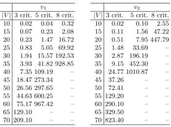
The experimentations on the Choquet optimal spanning tree problem (Cv-ST)
were performed on complete graphs (cliques). The criteria values on each edge are randomly drawn between 1 and 100. The number of criteria is 3, 5 or 8, and the number of nodes ranges from 10 to 70. For each class of graphs (characterized by the number of nodes and the number of criteria), we solve 50 different instances. Table 1 summarizes the average execution times (in seconds) on these instances. Symbol “–” means that the average execution times exceed 30 minutes.
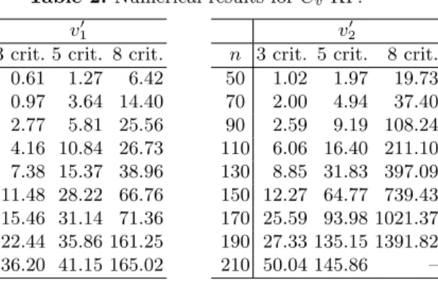
The experimentations on the Choquet optimal 0-1 knapsack problem (Cv-ST)
were also performed on 50 different instances for each category. Table 2 shows com-putation times (in sec) obtained on at least 30 different instances for each size, with profits and weights randomly drawn between 1 and 100, and a maximum weight capacity W equal to 50% of the total weight of the items. The number of items ranges from 50 to 210. Here again, the number of criteria is 3, 5 or 8.
Table 1. Numerical results for Cv-ST.
v1
|V | 3 crit. 5 crit. 8 crit. 10 0.02 0.04 0.32 15 0.07 0.23 2.08 20 0.23 1.47 16.72 25 0.83 5.05 69.92 30 1.94 15.57 192.53 35 3.93 41.82 928.85 40 7.35 109.19 – 45 18.47 273.34 – 50 26.56 297.65 – 55 44.63 600.25 – 60 75.17 967.42 – 65 129.10 – – 70 209.10 – – v2
|V | 3 crit. 5 crit. 8 crit. 10 0.02 0.10 2.55 15 0.11 1.56 47.22 20 0.51 7.95 447.79 25 1.48 33.69 – 30 2.87 196.19 – 35 9.15 452.30 – 40 24.77 1010.87 – 45 37.26 – – 50 72.41 – – 55 129.20 – – 60 290.10 – – 65 329.50 – – 70 823.40 – –
These results show the efficiency of the branch and bound procedures. For exam-ple, when capacity v01 is used, it takes only one minute for solving problem Cv-KP
with 150 items and 8 criteria, and only two minutes for solving problem Cv-ST with
Table 2. Numerical results for Cv-KP.
v10
n 3 crit. 5 crit. 8 crit. 50 0.61 1.27 6.42 70 0.97 3.64 14.40 90 2.77 5.81 25.56 110 4.16 10.84 26.73 130 7.38 15.37 38.96 150 11.48 28.22 66.76 170 15.46 31.14 71.36 190 22.44 35.86 161.25 210 36.20 41.15 165.02 v02
n 3 crit. 5 crit. 8 crit. 50 1.02 1.97 19.73 70 2.00 4.94 37.40 90 2.59 9.19 108.24 110 6.06 16.40 211.10 130 8.85 31.83 397.09 150 12.27 64.77 739.43 170 25.59 93.98 1021.37 190 27.33 135.15 1391.82 210 50.04 145.86 –
times depend on the capacity. In particular the times are better with capacity v1
(resp. v10) than with capacity v2 (resp. v02). We might explain this observation by
remarking that v2and v20 are monotone of infinite order, but a more thorough study
would be necessary to confirm this tentative explanation.
5 Conclusion
We have presented a general bound that can be used for the search for Choquet-optimal solutions in combinatorial problems. This bound is valid for any multiobjec-tive optimization problem provided we chose a submodular capacity in minization (resp. a supermodular capacity for maximization) so as to reflect preference for interior points. Given a set of criteria weights (ω1, . . . , ωq), a possible example of
suitable capacity is given by v(A) = ϕ(P
i∈Aωi) for all A ⊆ Q which is
supermod-ular whenever ϕ(x) ≤ x and submodsupermod-ular whenever ϕ(x) ≥ x. Interestingly enough, the Choquet integral used with such a capacity is nothing else but the weighted or-dered weighted averaging operator (WOWA) consior-dered by Ogryczak and Sliwinski (2007) for compromise search in continuous multiobjective optimization problems. WOWA operator, also known as Yaari’s model in Economics (Yaari, 1987), is there-fore a particular case of Choquet integral. Hence, the bound we introduced in this paper might be used as well to determine WOWA-optimal operators on combinato-rial domains provided ϕ is compatible with preference for interior points. Conversely, the work of Ogryczak and Sliwinski (2007) for WOWA-optimization on continuous domains should provide alternative bounds for Cv-KP by relaxing the integrality
constraint.
References
Chateauneuf, A. and Tallon, J. (2002). Diversification, convex preferences and non-empty core in the choquet expected utlity model. Economic Theory , 19, 509–523. Choquet, G. (1953). Theory of capacities. Annales de l’Institut Fourier , 5, 131–295.
Ehrgott, M. (2005). Multicriteria Optimization. 2nd ed. Springer-Verlag.
Galand, L. and Perny, P. (2007). Search for Choquet-optimal paths under uncer-tainty. In Proceedings of the 23rd conference on Uncertainty in Artificial Intelli-gence, pages 125–132, Vancouver, Canada. AAAI Press.
Galand, L. and Spanjaard, O. (2007). OWA-based search in state space graphs with multiple cost functions. In 20th International Florida Artificial Intelligence Research Society Conference, pages 86–91. AAAI Press.
Grabisch, M., Murofushi, T., and Sugeno, M. (2000). Fuzzy measures and integrals. Theory and applications. Studies in Fuzziness, Physica Verlag.
Hamacher, H. and Ruhe, G. (1994). On spanning tree problems with multiple ob-jectives. Annals of Operations Research, 52, 209–230.
Kappel, F. and Kuntsevich, A. (2000). An implementation of Shor’s r-algorithm. Computational Optimization and Applications, 15, 193–205.
Martello, S. and Toth, P. (1975). An upper bound for the zero-one knapsack problem and a branch and bound algorithm. European Journal of Operational Research, 1, 169–175.
Murthy, I. and Her, S. (1992). Solving min-max shortest-path problems on a network. Naval Research Logistics, 39, 669–683.
Ogryczak, W. and Sliwinski, T. (2007). On optimization of the importance weighted OWA aggregation of multiple criteria. In Computational Science and Its Appli-cations – ICCSA 2007 , pages 804–817. Lecture Notes in Computer Science. Perny, P., Spanjaard, O., and Storme, L.-X. (2007). State space search for risk-averse
agents. In Twentieth International Joint Conference on Artificial Intelligence, pages 2353–2358.
Punnen, A. and Aneja, Y. (1995). Minmax combinatorial optimization. European Journal of Operational Research, 81(3), 634–643.
Rosinger, E. E. (1991). Beyond preference information based multiple criteria deci-sion making. European Journal of Operational Research, 53(2), 217–227. Schmeidler, D. (1986). Integral representation without additivity. Proceedings of the
American Mathematical Society , 97(2), 255–261.
Shafer, G. (1976). A Mathematical Theory of Evidence. Princeton University Press. Shapley, L. (1971). Cores of convex games. International Journal of Game Theory ,
1, 11–22.