HAL Id: hal-01242826
https://hal-amu.archives-ouvertes.fr/hal-01242826
Submitted on 14 Dec 2015
HAL is a multi-disciplinary open access
archive for the deposit and dissemination of
sci-entific research documents, whether they are
pub-lished or not. The documents may come from
teaching and research institutions in France or
abroad, or from public or private research centers.
L’archive ouverte pluridisciplinaire HAL, est
destinée au dépôt et à la diffusion de documents
scientifiques de niveau recherche, publiés ou non,
émanant des établissements d’enseignement et de
recherche français ou étrangers, des laboratoires
publics ou privés.
A Connectivity-Based Eco-Regionalization Method of
the Mediterranean Sea
L. Berline, Anna-Maria Rammou, Andrea Doglioli, Anne Molcard, Anne
Petrenko
To cite this version:
L. Berline, Anna-Maria Rammou, Andrea Doglioli, Anne Molcard, Anne Petrenko. A
Connectivity-Based Eco-Regionalization Method of the Mediterranean Sea. PLoS ONE, Public Library of Science,
2014, 9 (e111978 ), �10.1371/journal.pone.0111978�. �hal-01242826�
Mediterranean Sea
Le´o Berline1,3,4*, Anna-Maria Rammou2, Andrea Doglioli2, Anne Molcard1, Anne Petrenko2
1 Universite´ du Sud Toulon-Var, Aix-Marseille Universite´, CNRS/INSU/IRD, Mediterranean Institute of Oceanography (MIO), La Garde, France, 2 Aix-Marseille Universite´, CNRS/INSU/IRD, Mediterranean Institute of Oceanography (MIO), Marseille, France,3 CNRS, Laboratoire d’Oce´anographie de Villefranche, Villefranche-sur-Mer, France, 4 Universite´ Pierre et Marie Curie, Paris 6, Laboratoire d’Oce´anographie de Villefranche, Villefranche-sur-Mer, France
Abstract
Ecoregionalization of the ocean is a necessary step for spatial management of marine resources. Previous ecoregionalization efforts were based either on the distribution of species or on the distribution of physical and biogeochemical properties. These approaches ignore the dispersal of species by oceanic circulation that can connect regions and isolates others. This dispersal effect can be quantified through connectivity that is the probability, or time of transport between distinct regions. Here a new regionalization method based on a connectivity approach is described and applied to the Mediterranean Sea. This method is based on an ensemble of Lagrangian particle numerical simulations using ocean model outputs at 1/12u resolution. The domain is divided into square subregions of 50 km size. Then particle trajectories are used to quantify the oceanographic distance between each subregions, here defined as the mean connection time. Finally the oceanographic distance matrix is used as a basis for a hierarchical clustering. 22 regions are retained and discussed together with a quantification of the stability of boundaries between regions. Identified regions are generally consistent with the general circulation with boundaries located along current jets or surrounding gyres patterns. Regions are discussed in the light of existing ecoregionalizations and available knowledge on plankton distributions. This objective method complements static regionalization approaches based on the environmental niche concept and can be applied to any oceanic region at any scale.
Citation: Berline L, Rammou A-M, Doglioli A, Molcard A, Petrenko A (2014) A Connectivity-Based Eco-Regionalization Method of the Mediterranean Sea. PLoS ONE 9(11): e111978. doi:10.1371/journal.pone.0111978
Editor: Brian R. MacKenzie, Technical University of Denmark, Denmark
Received December 9, 2013; Accepted October 10, 2014; Published November 6, 2014
Copyright: ß 2014 Berline et al. This is an open-access article distributed under the terms of the Creative Commons Attribution License, which permits unrestricted use, distribution, and reproduction in any medium, provided the original author and source are credited.
Funding: The research leading to these results has received funding from the European Community’s Seventh Framework Programme (FP7/2007–2013) under Grant Agreement No. 287844 for the project ‘‘Towards COast to COast NETworks of marine protected areas (from the shore to the high and deep sea), coupled with sea-based wind energy potential’’ (COCONET). The funders had no role in study design, data collection and analysis, decision to publish, or preparation of the manuscript.
Competing Interests: The authors have declared that no competing interests exist. * Email: [email protected]
Introduction
The ecoregionalization of the ocean is useful for scientific research, conservation and management of the marine environ-ment and marine resources. For instance, ecoregionalization is needed to extrapolate punctual or transect data to broader areas and to target specific regions for interdisciplinary research (as in the Mediterranean Sea, [1]). Conservation and management goals range from selecting areas to protect [2] to defining fisheries zones or zones for monitoring and mitigating marine pollution.
To date, several approaches of ecoregionalization were used depending on the data at hand [3]. The taxonomic approach is based on species distributions and identifies areas of broadly similar assemblage of species [4–6]. The ecological approach is based on habitat characteristics; it separates areas of similar seasonal cycles of physical and biogeochemical variables [7–10]. This approach benefited from the nearly continuous coverage of satellite data. Lastly, the integrative approach is a combination of both taxonomic and ecological approaches that takes into account both the habitat and the species inhabiting it [11].
However, in the marine environment the species distribution not only results from selection by the local environment but also from dispersal of propagules and adults organisms (e.g. the metapopulation
concept of Levins [12,13]). Therefore an ecoregionalization based on dispersal by ocean circulation is needed; recent studies start taking into account dispersal in defining management units [14]. However it was never achieved quantitatively at basin scale. Today this is possible, as widely available ocean circulation models provide 3 dimensional, time varying, realistic and consistent depictions of oceanic currents at basin scale. The goal of this paper is to present a regionalization method based on connectivity, assessed from ensemble Lagrangian simulations using ocean circulation model velocity outputs.
This method is applied to the Mediterranean basin, which is a target region for spatial planning owing to its high level of endemism and high biodiversity [15]. Surface circulation shows a complex pattern of larger and smaller gyres, driven by the entrance of Atlantic water at Gibraltar Strait [1], local meteorol-ogy and bathymetry. The oligotrophy increases toward the East, but productive spots also exist over shelves and deep mixing areas, thus creating a significant heterogeneity in ecosystem functioning and habitats.
Materials and Methods
The general outline of the method is as follow (Fig. 1): Lagrangian trajectories are computed from ocean circulation
model velocity outputs for particles seeded over the whole model domain at three depths (0.5 m, 50 m and 100 m). The domain is divided into a regular grid (hereinafter connectivity grid) and the trajectories are used to derive the mean connection time between every pair of grid cell. In this way a mean connection time matrix is obtained and then transformed into an oceanographic distance matrix, used as input to a hierarchical clustering algorithm. Finally clustering produces a partition of the domain.
Daily outputs velocity fields for four years (2007–2010) were taken from the configuration PSY2V3 of the operational system MERCATOR OCEAN [16]. The PSY2V3 configuration covers the North Atlantic ocean and Mediterranean Sea, and is based on the NEMO-OPA primitive equations code [17] with assimilation of observed data (satellite and in situ). Here, only the domain subset covering the Mediterranean Sea was used. Daily surface forcing are provided by ECMWF [18]. The velocity components are distributed in an Arakawa C type grid [19]. The horizontal resolution is 1/12u (,8 km) and there are 50 fixed vertical levels with higher resolution at the surface. The vertical mixing is described by a TKE closure scheme [20] and the advection by a TVD 2nd order centered scheme [21].
The trajectories followed by numerical particles were calculated offline with the Lagrangian diagnostic tool ARIANE [22]. The trajectories only result from the horizontal advection at three depths (0.5 m hereinafter called surface, 50 m and 100 m) chosen to represent the transport in the epipelagic layer. No vertical velocity was considered to keep particles in the 0–100 m range. The one year integration time was chosen to allow particles to cover the whole basin and therefore quantify basin scale connectivity and to keep computation time reasonable. Particles were seeded every 10 km on a regular square grid covering the whole domain, totaling 25,646 initial positions for surface depth and 23,770 for depths 50 and 100 m because the domain is smaller. Particles were seeded every 3 days from the 1st to the 25th of every month, from January 1st2007 to December 25st2009 in order to fully sample the variability of the circulation. This represents a total of 8,309,304 particles for surface depth, respectively 7,701,480 for depths 50 and 100 m. The choice of 10 km and 3 days is a compromise between matching the horizontal resolution of the model, taking into account mesoscale processes and keeping an affordable computing time of resulting trajectories. We thus obtained three ensembles of trajectories, one per depth.
In order to quantify the connections over the model domain, the domain was divided into grid cells of 50 km650 km on a regular square grid, the connectivity grid, with a total of 1095 cells covering only regions with depths greater than 100 m. The 50 km resolution is sufficient to keep a reasonably realistic coastline while being suitable with the seeding density chosen. Thus each connectivity grid cell contains 5*5 = 25 particles for each initial seeding date, except grid cells including land that contains less particles.
To quantify the connectivity between each grid cell, we used the Mean Connection Time, hereinafter MCT. Defining T(i,j) as the transit time from grid celli to grid cell j, MCT(i,j) was computed as
MCT i,jð Þ~1 M X n~M n~1 Tnði, jÞ
M being the number of particle transitioning from i to j. Note that for each trajectory, all intermediate transitions were used to compute the MCT. The sensitivity of MCT to the number of
particles was tested. The suite of MCT matrices converged when the number of particles was greater than 6,000,000, therefore we considered that 8,309,304 particles and respectively 7,701,480 particles for depths 50 and 100 m were sufficient to obtain a robust MCT matrix. Moreover, to keep MCT robust, it was computed only whenM was greater or equal to 50. Four MCT matrices of size 109561095 were computed: one MCT matrix from each ensemble of trajectories (MCT0, MCT50, MCT100for
0.5, 50 and 100 m depths trajectories respectively) and also one MCT matrix using the three ensembles together (MCT3depths).
Not all grid cells of the domain were connected within one year, especially remote cells (e.g. Northern Aegean and Gibraltar Strait). Thus the resulting MCT matrices had gaps (from 37% to 56%). These gaps are a problem for the steps of computing the oceanographic distance and applying hierarchical clustering on it. Therefore a gap filling procedure was introduced as follows (see Appendix S1):
#For each unconnected pair of grid cells i-j, we looked for grid
cells k so that i-k and k-j pairs are connected. There must be at least 50 grid cells k as forM.
#Then we computed MCT(i,j) for pair i-j as the sum of the
MCT(i,k) and MCT(k,j), averaged on all existing cells k, and filled the MCT(i,j) value in the matrix.
After 3 iterations of this procedure, each MCT matrix was filled. The resulting MCT values ranged from 10 days to 3000 days. This gap filling procedure avoided the very long integration time (.8 years) needed if we were to fill the whole MCT matrices from original trajectories alone.
This led to four full MCT matrices, which are asymmetric since the time to go fromi to j is not equal to the time to go from j to i. Then the oceanographic distance (OD) was defined after [23] as the minimum of the two MCT values associated to each pair of grid cellsi and j (travel from i to j and return travel from j to i). We chose the minimum value as it corresponds to the fastest route of transport which is also the shortest in length.
OD i,jð Þ~ min MCT i,jð ð Þ,MCT j,ið ÞÞ
This gave four symmetric matrices, (OD0, OD50, OD100,
OD3depths) where all diagonal terms (autoconnection time) were set
to zero.
Finally hierarchical clustering analysis was applied on each of the oceanographic distance matrix. This method has proved to be robust in the classification of atmospheric wind data (e.g. [24]) and hydrological data (e.g. [25]). Hierarchical clustering assigns grid cells to different clusters in a way that each grid cell belongs to only one cluster [26], and each cluster belongs to a larger cluster (Fig. 2). The grid cells are grouped according to their similarity, which here is the oceanographic distance. Thus there is no distance metric applied as in usual clustering exercises. During each sequence of the clustering algorithm, the distances between the new clusters formed and the other grid cells are computed. This step requires a linkage criterion to be defined. Here we used the flexible [27] and Ward linkages [28]. WPGMA linkage was also tested ([27]) but flexible and Ward best balanced the dendrogram. For a given cut-off level of the dendrogram, we obtained a partition of the grid cells in a certain number of clusters, which is, in the spatial domain, a regionalization. Each cluster corresponded to a region on the connectivity grid whose contours were identified. Finally for each cluster, the within-cluster MCT was computed and plotted as a function of the number of clusters from 2 to 31 (Fig. 3).
Our ‘‘best estimate’’ regionalization was computed using flexible link and the matrix OD3depths, built from the complete
ensemble of trajectories (Fig. 4). We also computed one region-alization for each of the three depths and two linkages (6 cases). To assess the sensitivity of the regionalization results to the linkage and depth used, we computed the boundary stability, which is simply the local frequency of occurrence of a boundary in the spatial domain among the 6 cases, as defined in [29].
The choice of the optimal cut-off level and number of cluster is not straightforward here, because the distance matrix (OD) is not
computed with a distance metric applied to a given dataset. Thus, usual criteria based on dataset variance within clusters cannot be used (e.g. [30]) because there is no dataset. Instead we took a simple approach comparing results from Ward and flexible linkage. For each partition into n clusters, we compute the proportion of cells classified in the same cluster with Ward and flexible (see Appendix S2). This proportion increases from 82%, to 88% from for n = 2 to n = 6 clusters, then drops to values ,70% for n.6. Therefore we consider that the optimal cluster number is 6 as it gives more information while keeping consistent results
Figure 1. Schematic of the steps of the regionalization method. Note that steps 2 to 5 are repeated using trajectories at the 3 depths separately, shown with the three arrows, and then using them altogether.
among the two linkages. However, as no absolute criterion is available, we show the maximum number of clusters that we can interpret, which is 22 clusters. The clusters above 22 require detailed regional information to be interpreted, which is beyond the scope of this study.
Results
When the number of clusters increases, the within-cluster MCT diminishes, as well as the size of each region (Figs. 3 and 4). The average MCT ranges from 188 days for 2 clusters to ca. 90 days for 22 clusters.
On the basis of our interpretation of regions with respect to circulation, we retained 22 clusters (Fig. 4). The boundaries of each region were identified and colored according to the number of cluster obtained varying the cutoff distance from 10,000 (2 clusters) to 507 (22 clusters). The boundary #1 partly cuts the Sicily Strait (Fig. 4) and separates the Western and Eastern basins. The boundary #2 isolates Levantine basin from Ionian Sea and Adriatic Sea. The boundary #3 isolates the northern Ionian and Adriatic Sea from Southern Ionian. Then boundary #4 separates the Western basin into a western and an eastern part. The boundary #5 isolates the Levantine basin plus a part of AW current off Lybia from the Aegean Sea. The boundary stability map (Fig. 5) shows that some of the boundaries shown on Fig. 4 are stable (e.g. boundary #7, 11, 16) while others are variable in
position or occurrence (e.g. boundary #4). Also, some boundaries (e.g. #2, 6, 8) have only a portion that is stable.
Then considering the 22 regions, the Western basin is separated into eight regions; regions A and B in the Northern part of the basin, G, F and E in the South and C, D that contains the Tyrrhenian sub-basin, region H at the center. In the Eastern basin, the Adriatic Sea is one region I. The Ionian Sea is separated into regions J, V, T at the center and K to the east, with U and S along the coasts of Libya and Tunisia. The Aegean Sea is divided into two regions, M in the East, L in the West. The Levantine basin has four regions: two coastal regions N and O, one southern region P and one center region Q. Considering only stable boundaries, the Western basin only has 5 regions. The Eastern basin has few continuous boundaries, only 4 regions are delimited (Adriatic, South of Sicily Strait and regions U and O).
Discussion
The boundary stability shows that the majority but not all boundaries are robust to changes in linkages and depths. Often, linkages or depth changes can produce minor shifts in boundary position, hence reducing boundary stability as defined here. When a boundary is not stable, it means that either the circulation is variable, either it is located in a region where the distance (OD) among grid cells is small thus the boundary position varies according to the overall content of each cluster. Thus the
Figure 2. Cluster dendrogram of the oceanographic distance matrix OD3depthsusing the flexible linkage. Horizontal black lines show
the cut-off values for 3 and 22 clusters. doi:10.1371/journal.pone.0111978.g002
boundary map must be analyzed jointly with the boundary stability to assess our regionalization.
1. Regions reveal circulation patterns
First the meaning of the regions obtained needs to be explained. One region contains grid cells that are connected at shorter time scale with each other than they are to the grid cells of the other regions. In the following, the relationship between the clusters boundaries, their stability and the circulation is examined in detail in comparison with the model average velocity fields (Fig. 4) and literature.
The hierarchy of cluster boundary is in good agreement with the surface general circulation scheme proposed by Millot et al. [31], their figure 2. Boundary #1 separates the Western and Eastern basins at the Sicily strait, boundary #2 isolates the Eastern Levantine, then boundary #3 the Adriatic Sea together with the northern part of the Ionian. Boundaries are often parallel to the mean velocity field. For instance boundary #16 is parallel to the Northern Current, boundary #11 parallel to the Asia Minor Current. Boundary can also separate two currents branches (the ATC along Tunisia and the AIS along Sicily, for part of boundaries #1 and 10, see [32]). This illustrates the barrier role of semi-permanent jets in the ocean. However, this is not always
the case (e.g. boundary #1 at the Sicily Strait, boundary #18 at Oranto Strait). This can occur as the MCT matrix was computed from the time varying flow field, not from the mean field shown here and because each cluster is separated according to its overall distance with other clusters.
In the Western basin, boundary #16 is associated to the path of the Northern Current [31] and is the most stable. The boundary #6 from Spain to the Baleares follows approximately the Balearic front and is also rather stable. The Tyrrhenian Sea contains regions B, C, D with partly stable boundaries. Region C east of the Strait of Bonifacio contains the wind induced cold recirculation identified by [31], which is a potential dense water formation zone [33]. The Southern region G is restricted to the Alboran Sea.
In the Eastern basin, the Ionian Sea has two Southern regions U and S. Boundary #10 follows the Sicilian current of AW and region U contains the area of accumulation of eddies of the Ionian Sea [31]. The region V can correspond to the meandering stream identified by [34] or considered as interannual variability by [31]. The South-eastern Levantine has a region O with a stable boundary #7. Region O corresponds to the eddy accumulation zone gLE following [35]. The Asia Minor current along the Southern coasts of Turkey is captured in region N and has a stable boundary #11. Finally, the Aegean Sea is divided into an Eastern
Figure 3. Within cluster mean connection time as a function of the cluster number for MCT3depths. White dots are the mean for each
cluster, black dots are the mean over all clusters. doi:10.1371/journal.pone.0111978.g003
region M fed by AW and a North-Western region L fed by Black Sea outflow waters.
Some regions are virgin of any boundaries (Fig. 5), like the center of Gulf of Lion, the Alboran Sea, the Eastern Tyrrhenian Sea, the Northern Adriatic Sea, South of Greece, the South-East of the Levantine basin. This means that these regions are intraconnected at a time scale of less than ca 90 days (see Fig. 3). Thus this regionalization reveals known circulation patterns and summarizes them in a way that complements the simple average velocity field analysis. It can be used to quantitatively compare the circulation patterns from contrasted periods or from different models.
2. Some boundaries coincide with major environmental boundaries and range limits of zooplankton assemblages
The identification of regions close to each other, not geograph-ically but in terms of oceanographic connections, should help understanding the spatial distribution of properties that are passively transported by currents, such as conservative physical properties, or planktonic organisms living in the surface layer (epipelagic).
First, boundaries emerging from circulation alone often match major discontinuities in variables describing the environment. For instance a strong latitudinal salinity gradient exists near the Balearic Islands, close to our boundary #6. However, our
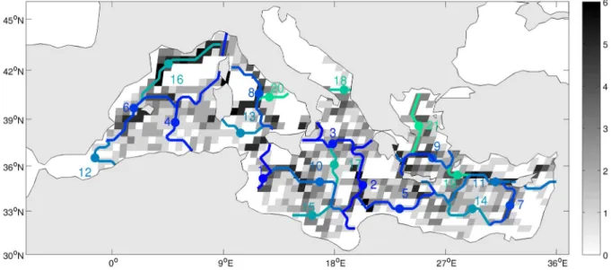
Figure 5. Map of the boundary stability (gray scale) derived from the 6 cases of clustering (3 depths62 linkages). Boundary stability is defined as the number of occurrence of a boundary in each grid cell among the 6 cases. Boundaries are overlaid as in figure 4.
doi:10.1371/journal.pone.0111978.g005
Figure 4. Map of the 21 clusters boundaries obtained from clustering of the oceanographic distance matrix OD3depthsusing the
flexible link. Each boundary is colored and numbered according to the cut-off distance on the dendrogram (from blue – high distance- to green-low distance). Each region is identified by a letter from A to V. The velocity from the circulation model, averaged for the 4-year (2007–2010) and the 3 depths is overlaid as black vectors.
doi:10.1371/journal.pone.0111978.g004
boundary #6 coincides with the Balearic Current but not to the Balearic salinity front, located more to the South [36]. Our boundary #16 coincides with a temperature and salinity front in the Ligurian Sea, and also in phytoplankton biomass (Fig. 1 in [10]). Off the Catalan coast, boundary #16 is consistent with the alongshore distribution of fish larvae [37], although located more offshore. Also, boundary #18 south of Adriatic Sea coincides with salinity fronts as seen in MEDATLAS [38]. This results from the dynamic links between density gradients and surface currents. The boundary #21 found in the Aegean Sea parallels the front in phytoplankton biomass [10]. At the Sicily strait, corresponding to our boundary #1, a boundary was also found by [9] (their figure 2) based on a clustering of sea surface temperature and ocean color data.
Within our regions, planktonic organisms are connected at shorter time scales than between regions. Thus hydrodynamical boundaries can become faunistic boundaries as suggested by Gaylord and Gaines [39] for larvae of benthic organisms. Given the spatial resolution, the MCT can correctly resolve connections of plankton organisms with a life cycle greater than 10 days, such as most zooplankton species [40]. Indeed, consistent with boundary #6 north of the Balearic Islands, a boundary exists between Atlantic zooplankton species to the South and Mediter-ranean species to the North [41,42]. Also, consistent with our boundaries #1 and #2, differences in zooplankton species composition between Eastern and Western basin were reported by several authors ([43] and references therein, [44]) although the spatial resolution of zooplankton data is generally not sufficient for accurately locating boundaries.
Ecoregions drawn qualitatively from expert knowledge of species assemblages ([45] their figure 2) also distinguish Atlantic-water regions including our region G, a Northern Current region including our region A, three Adriatic regions, one Aegean Sea region including our regions L and M, and two large zonal Eastern basin regions mostly consistent with boundaries #5 and #11.
However, for living organisms such as zooplankton, circulation alone is not sufficient to explain the distribution of a given species as it is adapted to its environment, in particular to a temperature range, e.g. [46]. Thus within our connected regions environmental conditions will restrict a species distribution to its specific preferendum, i.e. its ecological niche. Moreover, we deal with particles in the 0–100 m layer, which only properly represent epipelagic zooplankters dispersal.
3. How to use this regionalization?
To use this regionalization, the question of the number of clusters to retain will arise. With our approach, no existing criterion is available to define the optimal number. However the number of clusters can be chosen based on the time scale we are interested in, as regions isolated at a given time scale become connected at a larger time scale. Therefore the time scale of interest defines the appropriate cut-off distance and the resulting cluster number and sizes (Fig. 3). For instance, one can look for the scale of dispersal of planktonic larvae and hence consider the Pelagic Larval Duration (PLD) time scale. A PLD of 120 days (e.g. a crustacean as spiny lobster Palunirus elephas [47]) gives an adequate cluster number of ca 8. For a PLD of ca. 70 days (e.g. a labridae fish as Lipophrys trigloides [48) the adequate cluster number is ca 30. The lower bound time scale we can address with the present regionalization (,10 days) is set by the spatial resolution of our connectivity grid. Shorter time scales could be achieved with a finer connectivity grid.
Few existing studies can be compared to our regionalization because the approach is original. In the Mediterranean Sea,
Andrello et al. [49] obtained clusters of coastal marine protected areas (MPA) based on their connectivity assessed by Lagrangian simulations. Although the velocity fields, Lagrangian simulations set up and clustering method are different, we can compare the overall grouping obtained (their figure 5-A). Considering only clusters containing several MPAs (8 clusters out of 38), their clusters are mostly contained within single regions and do not spread across several regions. Exceptions occur in the Northern Ligurian Sea and Ionian Sea with MPAs located very close or even onto our regions’ boundaries. This probably results from the difference in the input velocity fields and subsequent connectivity quantification.
This new regionalization method quantifies the dispersal range of organisms, This dispersal dimension was shown to explain species distribution (e.g. [50]) and is thus critically needed [51]. This approach complements the usual regionalization methods rooted in the environmental niche concept (e.g. [9,10]). For instance, the Chl-a based regionalization from [10] reflects the regime of nutrients inputs and stratification, thus they are not directly linked to surface circulation patterns. Adding our connectivity-based regionalization helps understanding the types of environment that plankton is facing, through passive horizontal transport, vertical mixing and production processes. Practically, our OD matrices could be used as a constraint during the clustering of Chl-a, as for chronological clustering [52].
Also, our regions illustrate why plankton organisms may be encountered outside their optimum range (plankton expatriates, e.g. [53]) and where transport-driven fluctuations of plankton communities are expected. Indeed fluctuations of region bound-aries may produce large biogeographic fluctuations noticeable at fixed points (e.g. [54,55]). Regions can also help tracking invasions of exotic organisms, for instance the so-called lessepsian species coming from the Suez Canal [56]. Apart from living organisms, our regions could be used to quantify areas of dispersion of pollutants coming from ships or land sources [57].
Finally this regionalization is useful as a framework to interpret the genetic differentiation of a given species sampled throughout the Mediterranean (e.g. [58]). Further, our approach could be used to define a priori units for grouping existing MPA or set up new MPA (e.g. [59] for the Gulf of Lions), as envisioned in the EU Integrated Project COCONET (www.coconet-fp7.eu).
4. Perspectives
The regionalization proposed here will eventually be compared to an ongoing biogeochemistry-based regionalization [60], and to zooplankton species distribution as available in database COPE-PODS [61].
Concerning the methods, several points can be made. With a similar approach but shorter simulations, we can explore the seasonal variability of clusters boundaries that may be significant [62]. Here we used hierarchical clustering to extract clusters from the oceanographic distance, but clusters could also be computed with other methods such as graph theory that uses the asymmetry of the connectivity matrix (e.g. [49,63]). Finally, this method was applied to the Mediterranean Sea but it can be applied anywhere, at any spatial scales as long as accurate and long term model velocity outputs are available.
Supporting Information
Appendix S1 Method to fill the gap of the MCT matrix. (DOC)
Appendix S2 Method for choosing the optimal cut-off distance. (DOC)
Acknowledgments
Mercator-ocean (www.mercator-ocean.fr) is thanked for providing velocity outputs for configuration PSY2V3. Fabien Lombard is thanked for useful feedback on an earlier version of the manuscript. The two reviewers are thanked for their constructive comments.
Author Contributions
Conceived and designed the experiments: LB AMR AD AM. Performed the experiments: AMR LB. Analyzed the data: LB AMR. Wrote the paper: LB AMR AD AM AP.
References
1. Durrieu de Madron X, Guieu C, Sempere R, Conan P, Cossa D, et al. (2011) Marine ecosystems’ responses to climatic and anthropogenic forcings in the Mediterranean. Progress in Oceanography 91: 97–166.
2. Giakoumi S, Sini M, Gerovasileiou V, Mazor T, Beher J, et al. (2013) Ecoregion-Based Conservation Planning in the Mediterranean: Dealing with Large-Scale Heterogeneity. PLoS ONE 8(10): e76449. doi:10.1371/journal.pone.0076449. 3. UNESCO (2009) Global Open Oceans and Deep Seabed (GOODS)
Biogeo-graphic Classification. Paris. UNESCO-IOC. IOC Technical Series 84 92pp. 4. Forbes E (1856) Map of the distribution of marine life. in Johnston AK, editor.
The Physical Atlas of Natural Phenomena. Edinburgh (Scotland): William Blackwood and Sons. pp. 99–102.
5. Ekman S (1953) Zoogeography of the Sea. London: Sidgwick and Jackson. 417 p.
6. Briggs JC (1995) Global Biogeography. Amsterdam, Elsevier. 472 p. 7. Longhurst A (1995) Seasonal cycles of pelagic production and consumption.
Progress in Oceanography 36: 77–167.
8. Longhurst A (1998) Ecological geography of the sea Academic Press, London. 560 p.
9. Oliver MJ, Irwin AJ (2008) Objective global ocean biogeographic provinces. Geophysical Research Letters, 35, L15601, doi:101029/2008GL034238. 10. D’Ortenzio F, Ribera d’Alcala` M (2009) On the trophic regimes of the
Mediterranean sea: a satellite analysis. Biogeosciences 6: 139–148.
11. Koubbi P, Moteki M, Duhamel G, Goarant A, Hulley PA, et al. (2011) Ecoregionalization of myctophid fish in the Indian sector of the Southern Ocean: Results from generalized dissimilarity models. Deep Sea Research Part II: Topical Studies in Oceanography 58: 170–180.
12. Levins R (1969) Some demographic and genetic consequences of environmental heterogeneity for biological control. Bulletin of the Entomological Society of America 15: 237–240.
13. Obura D (2012) The Diversity and Biogeography of Western Indian Ocean Reef-Building Corals. PLoS ONE doi:10.1371/journal.pone.0045013. 14. Casale P, Mariani P (2014) The first ‘lost year’ of Mediterranean sea turtles:
dispersal patterns indicate subregional management units for conservation. Marine Ecology Progress Series 498: 263–274.
15. Coll M, Piroddi C, Steenbeek J, Kaschner K, Lasram F B, et al. (2010). The Biodiversity of the Mediterranean Sea: Estimates, Patterns, and Threats. PLoS ONE,5(8).
16. Bahurel P (2006) MERCATOR OCEAN global to regional ocean monitoring and forecasting. In: Chassignet, E P and Verron, J editors, Ocean Weather Forecasting Springer, Netherlands, pp. 381–395.
17. Madec G (2008) ‘‘NEMO ocean engine’’. Note du Pole de mode´lisation, Institut Pierre-Simon Laplace (IPSL), France, No 27 ISSN No 1288–1619, 367 p. 18. Uppala S, Kallberg PW, Simmons AJ, Andrae U, Da Costa V, et al. (2005) The
ERA-40 re-analysis. Q J R Meteorol Soc, 131: 2961–3012.
19. Mesinger F, Arakawa A, Kasahara A (1976) Numerical methods used in atmospheric models, vol 1 World Meteorological Organization, International Council of Scientific Unions 37 p.
20. Blanke B, Delecluse P (1993) Variability of the tropical Atlantic ocean simulated by a general circulation model with two different mixed layer physics. Journal of Physical Oceanography 23: 1363–1388.
21. Zalesak ST (1979) Fully multidimensional flux corrected transport algorithms for fluids. J Comput Phys 31: 335–362.
22. Blanke B, Raynaud S (1997) Kinematics of the Pacific Equatorial Undercurrent: An Eulerian and Lagrangian approach from GCM results. Journal of Physical Oceanography 27: 1038–1053.
23. Alberto F, Raimondi PT, Reed DC, Watson JR, Siegel DA, et al. (2011) Isolation by oceanographic distance explains genetic structure for Macrocystis pyrifera in the Santa Barbara Channel. Molecular Ecology, 20: 2543–2554. 24. Burlando M, Antonelli M, Ratto C (2008) Mesoscale wind climate analysis:
identification of anemological regions and wind regimes. Int J Climatol 28: 629– 641.
25. Hjelmervik KT, Hjelmervik K (2013) Estimating temperature and salinity profiles using empirical orthogonal functions and clustering on historical measurements. Ocean Dynamics 63: 809–821.
26. Legendre P, Rogers DJ (1972) Characters and clustering in taxonomy: a synthesis of two taximetric procedures. Taxon 567–606.
27. Lance GN, Williams WT (1967). A general theory of classificatory sorting strategies 1. Hierarchical systems. The computer journal, 9: 373–380. 28. Ward JH Jr (1963) Hierarchical Grouping to Optimize an Objective Function.
Journal of the American Statistical Association 58: 236–244.
29. Oliver MJ, Glenn S, Kohut JT, Irwin AJ, Schofield OM, et al. (2004), Bioinformatic approaches for objective detection of water masses on continental shelves, J Geophys Res, 109, C07S04, doi:10.1029/2003JC002072.
30. Calinski RB, Harabasz J (1974) A dendrite method for cluster analysis. Commun. Stat. 3: 1–27.
31. Millot C, Taupier-Letage I (2005) Circulation in the Mediterranean sea. In: The Mediterranean Sea, Springer, pp. 29–66.
32. Poulain PM, Zambianchi E (2007) Surface circulation in the central Mediterranean Sea as deduced from Lagrangian drifters in the 1990s. Continental Shelf Research 27(7): 981–1001.
33. Fuda JL, Etiope G, Millot C, Favali P, Calcara M, et al. (2002) Warming, salting and origin of the Tyrrhenian Deep Water (2002) Geophys. Res. Letters 29, doi:10.1029/2001GL014072.
34. Malanotte-Rizzoli P, Artale V, Borzelli-Eusebi GL, Brenner S, Crise A, et al. (2014) G.: Physical forcing and physical/biochemical variability of the Mediterranean Sea: a review of unresolved issues and directions for future research, Ocean Sciences 10: 281–322, doi:10.5194/os-10-281-2014. 35. Hamad N, Millot C, Taupier-Letage I (2005) A new hypothesis about the
surface circulation in the eastern basin of the Mediterranean sea. Progress in Oceanography 66: 287–298.
36. Mariani P, MacKenzie BR, Iudicone D, Bozec A (2010) Modelling retention and dispersion mechanisms of bluefin tuna eggs and larvae in the northwest Mediterranean Sea. Progress in Oceanography 86(1): 45–58.
37. Sabate´s A, Olivar MP, Salat J, Palomera I, Alemany F (2007) Physical and biological processes controlling the distribution of fish larvae in the NW Mediterranean. Progress in Oceanography, 74(2): 355–376.
38. Rixen M, Beckers JM, Brankart JM, Brasseur P (2001) A numerically efficient data analysis method with error map generation. Ocean Modelling 2: 45–60. 39. Gaylord B, Gaines SD (2000) Temperature or transport ? range limits in marine
species mediated solely by flow. The American Naturalist 155: 769–789. 40. Carlotti F, Poggiale JC (2010) Towards methodological approaches to
implement the zooplankton component in ‘‘end to end’’ food-web models. Progress in Oceanography, 84: 20–38.
41. Fernandez de Puelles ML, Pinot J-M, Valencia J (2003) Seasonal and interannual variability of zooplankton community in waters off Mallorca island (Balearic Sea, Western Mediterranean): 1994–1999. Oceanologica Acta 26: 673–686.
42. Fernandez de Puelles ML, Molinero JC (2007) North Atlantic climate control on plankton variability in the Balearic Sea, western Mediterranean. Geophysical Research Letters 34, L04608 doi:101029/2006GL028354.
43. Siokou-Frangou I, Christaki U, Mazzocchi MG, Montresor M, Ribera d’Alcala´ M, et al. (2010) Plankton in the open Mediterranean Sea: a review. Biogeosciences 7: 1543–1586, doi:105194/bg-7-1543-2010.
44. Nowaczyk A, Carlotti F, Thibault-Botha D, Pagano M (2011) Distribution of epipelagic metazooplankton across the Mediterranean Sea during the summer BOUM cruise. Biogeosciences, 8: 2159–2177, doi:105194/bg-8-2159-2011. 45. Bianchi C, Morri C (2000) Marine biodiversity of the Mediterranean Sea:
situation, problems and prospects for future research. Marine Pollution Bulletin 40: 367–376.
46. Beaugrand G (2005) Monitoring pelagic ecosystems using plankton indicators. ICES Journal of Marine Science 62: 333–338.
47. Queiroga H, Blanton J (2004) Interactions between behavior and physical forcing in the control of horizontal transport of decapods crustacean larvae. Advances in Marine Biology 47: 198–214.
48. McPherson E, Raventos N, (2006) Relationship between pelagic larval duration and geographic distribution of Mediterranean littoral fishes. Marine Ecology Progress Series 327: 257–265.
49. Andrello M, Mouillot D, Beuvier J, Albouy C, Thuiller W, et al. (2013) Low connectivity between mediterranean marine protected areas: a biophysical modeling approach for the dusky grouperEpinephelus marginatus. Plos One 8(7): e68564 doi:101371/journalpone0068564.
50. Wernberg T, Thomsen MS, Connell SD, Russell BD, Waters JM, et al. (2013) The Footprint of Continental-Scale Ocean Currents on the Biogeography of Seaweeds. PLoS ONE doi:10.1371/journal.pone.0080168.
51. Guisan W, Thuiller W (2005) Predicting species distribution: offering more than simple habitat models. Ecology Letters 8: 993–1009.
52. Legendre P, Dallot S, Legendre L (1985) Succession of species within a community: chronological clustering, with applications to marine and freshwater zooplankton. American Naturalist 125: 257–288.
53. Olli K, Wassmann P, Reigstad M, Ratkova TN, Arashkevich E, et al. (2007) The fate of production in the central Arctic Ocean – top-down regulation by zooplankton expatriates. Progress in Oceanography 72: 84–113.
54. Chiba S, Di Lorenzo E, Davis A, Keister JE, Taguchi B, et al. (2013) Large-scale climate control of zooplankton transport and biogeography in the Kuroshio Oyashio Extension region. Geophysical Research Letters 40: 5182–5187.
55. Berline L, Zakardjian B, Molcard A, Ourmie`res Y, Guihou K (2013) Modelling transport and stranding of jellyfish Pelagia noctiluca in the Mediterranean Marine Pollution Bulletin, 70: 90–99.
56. Jribi I, Bradai MN (2012) First record of the Lessepsian migrant species Lagocephalus sceleratus (Gmelin,1789) (Actinopterygii: Tetraodontidae) in the Central Mediterranean. BioInvasions Records 1: 49–52 doi:10.3391/ bir.2012.1.1.11.
57. Olita A, Cucco A, Simeone S, Ribotti A, Fazioli L, et al. (2012) Oil spill hazard and risk assessment for the shorelines of a Mediterranean coastal archipelago. Ocean & Coastal Management 57: 44–52.
58. Serra IA, Innocenti AM, Di Maida G, Calvo S, Migliaccio M, et al. (2010) Genetic structure in the Mediterranean seagrassPosidonia oceanica: disentan-gling past vicariance events from contemporary patterns of gene flow. Molecular Ecology 19: 557–68.
59. Guizien K, Belharet M, Marsaleix P, Guarini JM (2012) Using larval dispersal simulations for marine protected area design: Application to the Gulf of Lions
(northwest Mediterranean). Limnology and Oceanography, 57: 1099–1112 doi:10.4319/lo.2012.57.4.1099.
60. Reygondeau G, Irisson J-O, Guieu C, Gasparini S, Ayata S-D, et al. (2013) Toward a dynamic biogeochemical division of the Mediterranean Sea in a context of global climate change. EGU General Assembly 2013, Vienna, Austria, 07–12 April 2013. Available at: http://meetingorganizer.copernicus. org/EGU2013/EGU2013-10011.pdf.
61. O’Brien TD, Wiebe PH, Hay S (2010) ICES Zooplankton Status Report 2008/ 2009 ICES Cooperative Research Report No 307 152.
62. Pizzigali C, Rupolo V, Lombardi E, Blanke B (2007) Seasonal probability dispersion maps in the Mediterranean Sea obtained from the Mediterranean Forecasting System Eulerian velocity fields. Journal of Geophysical Research 112, C05012.
63. Treml EA, Halpin PN, Urban DL Pratson LF (2008) Modeling population connectivity by ocean currents, a graph-theoretic approach for marine conservation. Landscape Ecology 23: 19–36.