HAL Id: hal-01413394
https://hal.inria.fr/hal-01413394
Submitted on 9 Dec 2016
HAL is a multi-disciplinary open access
archive for the deposit and dissemination of sci-entific research documents, whether they are pub-lished or not. The documents may come from teaching and research institutions in France or abroad, or from public or private research centers.
L’archive ouverte pluridisciplinaire HAL, est destinée au dépôt et à la diffusion de documents scientifiques de niveau recherche, publiés ou non, émanant des établissements d’enseignement et de recherche français ou étrangers, des laboratoires publics ou privés.
adjoint MPI-parallel programs
Ala Taftaf, Laurent Hascoët
To cite this version:
Ala Taftaf, Laurent Hascoët. On the correct application of AD checkpointing to adjoint MPI-parallel programs. VII European Congress on Computational Methods in Applied Sciences and Engineering (ECCOMAS 2016), Jun 2016, Crete, Greece. �hal-01413394�
Crete Island, Greece, 5–10 June 2016
ON THE CORRECT APPLICATION OF AD CHECKPOINTING TO
ADJOINT MPI-PARALLEL PROGRAMS
A.Taftaf, L. Hasco¨et
INRIA, Sophia-Antipolis, France, {Elaa.Teftef, Laurent.Hascoet}@inria.fr
Keywords: Algorithmic Differentiation, Adjoint, Checkpointing, Message Passing, MPI Abstract. Checkpointing is a classical technique to mitigate the overhead of adjoint Al-gorithmic Differentiation (AD). In the context of source transformation AD with the Store-All approach, checkpointing reduces the peak memory consumption of the adjoint, at the cost of duplicate runs of selected pieces of the code. Checkpointing is vital for long run-time codes, which is the case of most MPI parallel applications. However, the presence of MPI communi-cations seriously restricts application of checkpointing.
In most attempts to apply checkpointing to adjoint MPI codes (the “popular” approach), a num-ber of restrictions apply on the form of communications that occur in the checkpointed piece of code. In many works, these restrictions are not explicit, and an application that does not respect these restrictions may produce erroneous code.
We propose techniques to apply checkpointing to adjoint MPI codes, that either do not suppose these restrictions, or explicit them so that the end users can verify their applicability. These techniques rely on both adapting the snapshot mechanism of checkpointing and on modifying the behavior of communication calls.
One technique is based on logging the values received, so that the duplicated communications need not take place. Although this technique completely lifts restrictions on checkpointing MPI codes, message logging makes it more costly than the popular approach. However, we can refine this technique to blend message logging and communications duplication whenever it is possible, so that the refined technique now encompasses the popular approach. We provide el-ements of proof of correction of our refined technique, i.e. that it preserves the semantics of the adjoint code and that it doesn’t introduce deadlocks.
1 INTRODUCTION
Adjoint algorithms, and in particular those obtained through the adjoint mode of Automatic Differentiation (AD) [1], are probably the most efficient way to obtain the gradient of a numer-ical simulation. Given a piece of code P , adjoint AD (with the “Store-All” approach) consists of two successive pieces of code. The first one, the “forward sweep”−→P computes the original values and stores in memory the overwritten variables needed to compute the gradients. The second one, the “backward sweep” ←P , computes the gradients, using the intermediate values− stored as needed. Primarily, i.e. before any form of program optimisation, the adjoint program is simply−→P followed by a←P .−
Many large-scale computational science applications are parallel programs based on Message-Passing, implemented for instance by using the MPI message passing library. We will call them “MPI programs”. MPI programs consist of one or more threads (called ”MPI processes”) that communicate through message exchanges.
In most attempts to apply checkpointing to adjoint MPI codes (the “popular” approach), a number of restrictions apply on the form of communications that occur in the checkpointed piece of code. In many works, these restrictions are not explicit, and an application that does not respect these restrictions may produce erroneous code.
We propose techniques to apply checkpointing to adjoint MPI codes, that either do not suppose these restrictions, or explicit them so that the end users can verify their applicability. These techniques rely on both adapting the snapshot mechanism of checkpointing and on modifying the behavior of communication calls.
isend
Process1:
send wait recv
Process 2:
recv send recv
isend
Process 1:
send wait recv
Process 2: recv send recv isend =wait send =recv wait=irecv
recv =send recv =send send = recv recv =send
⃗
P
P
P
⃗
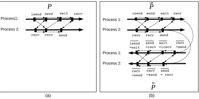
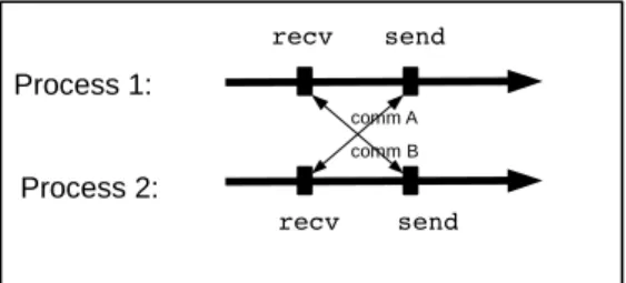
(a) (b) Process 1: Process 2:Figure 1: (a) Communications graph of an MPI parallel program with two processes. Thin arrows represent the edges of the communications graph and thick arrows represent the propagation of the original values by the processes. (b) Communications graph of the corresponding adjoint MPI parallel program. The two thick arrows in the top represent the forward sweep, propagating the values in the same order as the original program, and the two thick arrows in the bottom represent the backward sweep, propagating the gradients in the reverse order of the computation of the original values.
1.1 Communications graph of adjoint MPI programs
One commonly used model to study message-passing is the communications graph [[2], pp. 399403], which is a directed graph (see figure 1 (a)) in which the nodes are the MPI communication calls and the arrows are the dependencies between these calls. For simplicity, we omit the mpi prefix from subroutine names and omit parameters that are not essential in our context. Calls may be dependent because they have to be executed in sequence by a same process, or because they are matching send and recv calls in different processes.
• The arrow from each send to the matching recv (or to the wait of the matching isend) reflects that the recv (or the wait) cannot complete until the send is done. Similarly, the arrow from each recv to the matching send (or to the wait of the match-ing irecv) reflects that the send will block until the recv is done.
• The arrows between two successive MPI calls within the same process reflect the depen-dency due to the program execution order, i.e. instructions are executed sequentially. In the sequel, we will not show these arrows.
A central issue for correct MPI programs is to be deadlock free. Deadlocks are cycles in the communications graph.
There have been several works on the adjoint of MPI parallel programs [3],[4], [5], [6], [7]. When the original code performs an MPI communication call, the adjoint code must perform another MPI call, which we will call an “adjoint MPI call”.
• For instance the adjoint for a receiving call recv(b) is a send of the corresponding adjoint value b. In practice, this will write as send(b); b = 0.
• Symmetrically the adjoint for a sending call send(a) performs a receive of the corre-sponding adjoint value. In practice this will write as recv(tmp); a+ = temp.
This way, the adjoint code will perform a communication of the adjoint value (called “adjoint communication”) in the opposite direction of the communication of the primal value, which is what should be done according to the AD model. This creates in←P a new graph of communi-− cations (see figure 1 (b)), that has the same shape as the communications graph of the original program, except the inversion of the direction of arrows. This implies that if the communi-cations graph of the original program is acyclic, then the communicommuni-cations graph of ←P is also− acyclic. Since−→P is essentially a copy of P with the same communications structure, the com-munications graphs of−→P and←P are acyclic if the communications graph of P is acyclic. Since− we observe in addition that there is no communication from−→P to←P , we conclude that if P is− deadlock free, then P =−→P ;←P is also deadlock free.−
1.2 Checkpointing
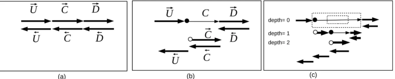
Storing all intermediate values in −→P consumes a lot of memory space. In the case of se-rial programs, the most popular solution is the “checkpointing” mechanism [8] (see figure 2). Checkpointing is best described as a transformation applied with respect to a piece of the orig-inal code (a “checkpointed part”). For instance figure 2 (a) and (b) illustrate checkpointing applied to the piece C of a code, consequently written as U ; C; D.
On the adjoint code of U ; C; D (see figure 2 (a)), checkpointing C means in the forward sweep not storing the intermediate values during the execution of C. As a consequence, the backward
D C ⃗ ⃗D C D ⃗ C C U ⃗ U U ⃗ ⃗ ⃗ ⃗ ⃗ ⃗ C ⃗D ⃗ U depth= 0 depth= 1 depth= 2 (a) (b) (c)
Figure 2: (a) A sequential adjoint program without checkpointing. (b) The same adjoint program with check-pointing applied to the part of code C. The thin arrow reflects that the first execution of the checkpointed code C does not store the intermediate values in the stack. (c) Application of the checkpointing mechanism on two nested checkpointed parts. The checkpointed parts are represented by dashed rectangles.
sweep can execute←D but lacks the stored values necessary to execute− ←C . To cope with that, the− code after checkpointing (see figure 2 (b)) runs the checkpointed piece again, this time storing the intermediate values. The backward sweep can then resume, with ←C then− ←U . In order to− execute C twice (actually C and later−→C ), one must store (a sufficient part of) the memory state before C and restore it before←C . This storage is called a snapshot, which we represent on fig-− ures as a • for taking a snapshot and as a ◦ for restoring it. Taking a snapshot “•” and restoring it “◦” have the effect of resetting a part of the machine state after “◦” to what it was immedi-ately before “•”. We will formalize and use this property in the demonstrations that follow. To summarize, for original code U ; C; D, whose adjoint is−→U ;−→C ;−→D ;←D ;− ←C ;− ←U , checkpointing C− transforms the adjoint into−→U ; •; C;−→D ;←D ; ◦;− −→C ;←C ;− ←U .−
The benefit of checkpointing is to reduce the peak size of the stack in which intermediate values are stored: without checkpointing, this peak size is attained at the end of the forward sweep, where the stack contains kU ⊕ kC ⊕ kD, where kX is the values stored by code X. In contrast,
the checkpointed code reaches two maximums kU⊕ kDafter
− → D and kU⊕ kCafter − → C . The cost of checkpointing is twofold: the snapshot must be stored, generally on the same stack, but its size is in general much smaller than kC. The othor part of the cost is that C is executed twice,
thus increasing run time.
1.3 Checkpointing on MPI adjoints
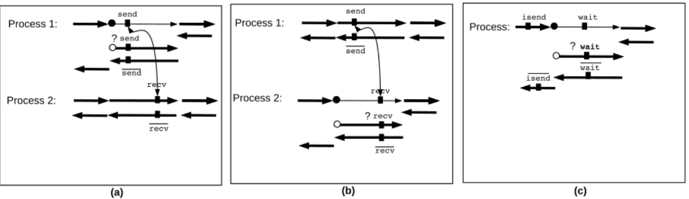
Checkpointing MPI parallel programs is restricted due to MPI communications. In previous works, the “popular” checkpointing approach has been applied in such a way that a check-pointed piece of code always contains both ends of each communication it performs. In other words, no MPI call inside the checkpointed part may communicate with an MPI call which is outside. Furthermore, non-blocking communication calls and their corresponding waits must be both inside or both outside of the checkpointed part. This restriction is often not explicitly mentioned. However, if only one end of a point to point communication is in the checkpointed part, then the above method will produce erroneous code. Consider the example of figure 3 (a), in which only the send is contained in the checkpointed part. The checkpointing mechanism duplicates the checkpointed part and thus duplicates the send. As the matching recv is not duplicated, the second send is blocked. The same problem arises if only the recv is contained in the checkpointed part (see figure 3 (b)). The duplicated recv is blocked. Figure 3 (c) shows the case of a non-blocking communication followed by its wait, and only the wait is con-tained in the checkpointed part. This code fails because the repeated wait does not correspond to any pending communication.
com-send recv send ? isend wait wait wait wait isend ? Process: (c) Process 1: Process 2: send recv recv send recv ? Process 2: Process 1: recv send (b) (a)
Figure 3: Three examples of careless application of checkpointing to MPI programs, leading to wrong code. For clarity, we separated processes: process 1 on top and process 2 at the bottom. In (a), an adjoint program after checkpointing a piece of code containing only the send part of point-to-point communication. In (b), an adjoint program after checkpointing a piece of code containing only the recv part of point-to-point communication. In (c), an adjoint program after checkpointing a piece of code containing a wait without its corresponding non blocking routine isend.
munications. These techniques either do not suppose restrictions on the form of communica-tions that occur in the checkpointed code, or explicit them so that the end user can verify their applicability. One technique is based on logging the values received, so that the duplicated communications need not take place. Although this technique completely lifts restrictions on checkpointing MPI codes, message logging makes it more costly than the popular approach. However, we can refine this technique to replace message logging with communications du-plication whenever it is possible, so that the refined technique now encompasses the popular approach. In section 2, we give a proof framework for correction of checkpointed MPI codes, that will give some sufficient conditions on the MPI adapted checkpointing technique so that the checkpointed code is correct. In section 3 , we introduce our MPI adapted checkpointing technique based on message logging. We prove that this technique respects the assumptions of section 2 and thus that it preserves the semantics of the adjoint code. In section 3, we show how this technique may be refined in order to reduce the number of values stored in memory. We prove that the refinement we propose respects the assumptions of section 2 and thus that it preserves the semantics of the adjoint code as well.
2 ELEMENTS OF PROOF
We propose adaptations of the checkpointing method to MPI adjoint codes, so that it provably preserves the semantics of the resulting adjoint code for any choice of the checkpointed part. To this end, we will first give a proof framework of correction of checkpointed MPI codes, that relies on some sufficient conditions on the MPI adapted checkpointing method so that the checkpointed code is correct.
On large codes, checkpointed codes are nested (see figure 2 (c)) , with a nesting level often as deep as the depth of the call tree. Still, nested checkpointed parts are obtained by repeated application of the simple pattern described in figure 2 (b). Specifically, checkpointing applies to any sequence of forward, then backward code (e.g. −→C ;←C on figure 2 (b)) independently of− the surrounding code. Therefore, it suffices to prove correctness of one elementary application of checkpointing to obtain correctness for every pattern of nested checkpointed parts.
To compare the semantics of the adjoint codes without and with checkpointing, we define the effect E of a program P as a function that, given an initial machine state σ, produces a
new machine state σnew = E (P, σ). The function E describes the semantics of P . It describes
the dependency of the program execution upon all of its inputs and specifies all the program execution results. The function E is naturally defined on the composition of programs by : E((P1; P2), σ) = E (P2, E (P1, σ)).
When P is in fact a parallel program, it consists of several processes pi run in parallel. Each
pimay execute point-to-point communication calls. We will define the effect E of one process p.
To this end, we need to specify more precisely the contents of the execution state σ for a given process, to represent the messages being sent and received by p. We will call “R” the (partly ordered) collection of messages that will be received (i.e. are expected) during the execution of p. Therefore R is a part of the state σ which is input to the execution of p, and it will be consumed by p. It may well be the case that R is in fact not available at the beginning of p. In real execution, messages will accumulate as they are being sent by other processes. However, we consider R as a part of the input state σ as it represents the communications that are expected by p. Symmetrically, we will call “S” the collection of messages that will be sent during the execution of p. Therefore, S is a part of the state σnewwhich is output by execution of p and it
is produced by p.
We must adapt the definition of E for the composition of programs accordingly. We explicit the components of σ as follows. The state σ contains:
• W , the values of variables
• R, the collection of messages expected, or “to be received” by p • S, the collection of messages emitted by p
With this shape of σ, the form of the semantic function E and the rule of the composition of pro-grams become more complex. Definition of E on one process p imposes the prefix Rpof R (the
messages to be received) that is required by p and that will be consumed by p. Therefore, the function E applies pattern matching on its R argument to isolate this “expected” part. Whatever remains in R is propagated to the output R. Similarly, SP denotes the suffix set of messages
emitted by p, to be added to S. Formally, we will write this as: E(p, hW, RP ⊕ R, Si) = hW0, R, S ⊕ SPi
To explicit the rule of code sequence, suppose that p runs pieces of code C and D in sequence, with C expecting incoming received messages RC and D expecting incoming received
mes-sages RD. Assuming that the effect of C on the state is:
E(C, hW, RC ⊕ R, Si) = hW0, R, S ⊕ SCi
and the effect of D on the state is: E(D, hW0, R
D ⊕ R, Si) = hW00, R, S ⊕ SDi,
then C; D expects received messages RC ⊕ RD (for the appropriate concatenation operator ⊕)
and its effect on the state is:
E(C; D, hW, RC⊕ RD⊕ R, Si) = hW00, R, S ⊕ SC ⊕ SDi.
Adjoint programs operate on two kinds of variables. On one hand, the variables of the original primal code are copied in the adjoint code. In the state σ, we will note their values “V ”. On the other hand, the adjoint code introduces new adjoint variables to hold the derivatives. In the state σ, we will denote their values “V ”.
Moreover, adjoint computations with the store-all approach use a stack to hold the intermediate values that are computed and pushed during the forward sweep−→P and that are popped and used during the backward sweep ←P . We will denote the stack as “k”. In the sequel, we will use a−
fundamental property of the stack mechanism of AD adjoints, which is that when a piece of code has the shape−→P ;←P , then the stack is the same before and after this piece of code. To be− complete, the state should also describe the sent and received messages corresponding to adjoint values (see section 1.1). As these parts of the state play a very minor role in the proofs, we will omit them. Therefore, we will finally split states σ of a given process as: σ = hV, V , k, R, Si. For our needs, we formalize some classical semantic properties of adjoint programs. These properties can be proved in general, but this is beyond the scope of this paper. We will consider these properties as axioms.
• Any “copied” piece of code X (for instance C) that occurs in the adjoint code operates only on the primal values V and on the R and S communication sets, but not on V nor on the stack. Formally, we will write:
E(X, hV, V , k, RX ⊕ R, Si) = hVnew, V , k, R, S ⊕ SXi, with the output Vnew and SX
depending only on V and on RX.
• Any “forward sweep” piece of code −→X (for instance −→U ,−→C or −→D ) works in the same manner as the original or copied piece X, except that it also pushes on the stack new values noted δkX, which only depend on V and RX. Formally, we will write:
E(−→X , hV, V , k, RX ⊕ R, Si) = hVnew, V , k ⊕ δkX, R, S ⊕ SXi
• Any “backward sweep” piece of code←X (for instance− ←U ,− ←C or− ←D ), on one hand operates− on the adjoint variables V and, on the other hand, uses exactly the top part of the stack δkX that was pushed by
− →
X . In the simplest AD model, δkX is used to restore the values
V that were held by the primal variables immediately before the corresponding forward sweep−→X . There exists a popular improvement in the AD model in which this restoration is only partial, restoring only a subset of V to their values before−→X . This improvement (called TBR) guarantees that the non-restored variables have no influence on the follow-ing adjoint computations and therefore need not be stored. The advantage of TBR is to reduce the size of the stack. Without loss of generality, we will assume in the sequel that the full restoration is used, i.e. no TBR is used. With the TBR mechanism, the semantics of the checkpointed program are preserved at least for the output V so that this proof is still valid. Formally, we will write:
E(←X , hV, V , k ⊕ δk− X, R, Si) = hVnew, Vnew, k, R, Si, where Vnewis equal to the value V
before running−→X (which is achieved by using δkX and V ) and Vnewdepends only on V ,
V and δkX.
• A “take snapshot” operation “•” for a checkpointed piece C does not modify V nor V , expects no received messages, and produces no sent messages. It adds into the stack enough values SnpC to permit a later re-execution of the checkpointed part. Formally,
we will write :
E(•, hV, V , k, R, Si) = hV, V , k ⊕ SnpC, R, Si, where SnpC is a subset of the values in
V , thus depending on only V .
• A “restore snapshot” operation “◦” of a checkpointed piece C does not modify V , expects no received messages and produces no sent messages. It pops from the stack the same set of values SnpC that the “take snapshot” operation pushed “onto” the stack. This modifies
V so that it holds the same values as before the “take snapshot” operation.
We introduce here the additional assumption that restoring the snapshot may (at least conceptually) add some messages to the output value of R. In particular:
Assumption 1. The duplicated recvs in the checkpointed part will produce the same values as their original calls.
Formally, we will write:
E(◦, hV, V , k ⊕ SnpC, R, Si) = hVnew, V , k, RC ⊕ R, Si where Vnew is the same as V
from the state input to the take snapshot.
Our goal is to demonstrate that the checkpointing mechanism preserves the semantics i.e.: Theorem 1. For any individual process p, for any checkpointed part C of p, (so that p = {U ;C:D}), for any state σ and for any checkpointing method that respects the Assumption 1:
E({−→U ;−→C ;→−D ;←D ;− ←C ;− ←U }, σ) = E ({− −→U , •, C,−→D ,←D , ◦,− −→C ,←C ,− ←U }, σ)−
Proof. We observe that the non-checkpointed adjoint and the checkpointed adjoint share a com-mon prefix−→U and also share a common suffix←C ;− ←U . Therefore, as far as semantics equivalence− is concerned, it suffices to compare−→C ;−→D ;←D with •, C,− −→D ,←D , ◦,− −→C .
Therefore, we want to show that for any initial state σ0 :
E({−→C ;−→D ;←D }, σ− 0) = E ({•, C,
− →
D ,←D , ◦,− −→C }, σ0)
Since the semantic function E performs pattern matching on the R0 part of its σ0 argument,
and the non-checkpointed code has the shape {−→C ;−→D ;←D }, R− 0matches the pattern RC⊕RD⊕R.
Therefore, what we need to show writes as:
E({−→C ;−→D ;←D }, hV− 0, V0, k0, RC⊕ RD ⊕ R, S0i) =
E({•, C,−→D ,←D , ◦,− −→C }, hV0, V0, k0, RC ⊕ RD ⊕ R, S0i)
We will call σ2, σ3 and σ6 the intermediate states produced by the non-checkpointed code (see
⃗
C
⃗
D
D
C
⃗
⃗
C
⃗
D
D
⃗
C
C
⃗
⃗
(a) (b) σ0 σ2 σ3 σ6 σ7 σ0 σ1' σ2' σ3' σ4' σ5' σ6' σ7'⃗
U
U
⃗
U
U
⃗
⃗
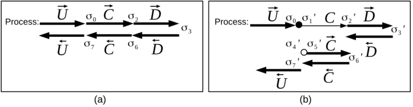
Process: Process:Figure 4: (a) An adjoint program run by one process. (b) The same adjoint after applying checkpointing to C. The figures show the locations (times) in the execution for the successive states σiand σi0.
figure 4 (a)). Similarly, we call σ01, σ02, σ30, σ40, σ50, σ60 the intermediate states of the checkpointed code (see figure 4 (b)). In other words: σ2 = E (
− → C , σ0); σ3 = E ( − → D , σ2); σ6 = E ( ←− D , σ3) and similarly σ10 = E (•, σ0); σ20 = E (C, σ10); σ03 = E ( − → D , σ20); σ04 = E (←D , σ− 30); σ50 = E (◦, σ04); σ60 = E (−→C , σ50).
Our goal is to show that σ60 = σ6. Considering first the non-checkpointed code, we propagate
the state σ by using the axioms already introduced: σ2 + E( − → C , σ0) = E ( − → C , hV0, V0, k0, RC ⊕ RD ⊕ R, S0i) = hV2, V0, k0⊕ δkC, RD⊕ R, S0⊕ SCi
with V2, SC and δkC depending only on V0and RC
σ3 + E( − → D , σ2) = E ( − → D , hV2, V0, k0⊕ δkC, RD⊕ R, S0⊕ SCi) = hV3, V0, k0 ⊕ δkC ⊕ δkD, R, S0⊕ SC⊕ SDi
with V3, SD and δkD depending only on V2and RD
σ6 + E( ←− D , σ3) = E ( ←− D , hV3, V0, k0⊕ δkC⊕ δkD, R, S0⊕ SC ⊕ SDi) = hV2, V6, k0⊕ δkC, R, S0⊕ SC ⊕ SDi
with V2and V6depending only on V3, V0and δkD
Considering now the checkpointed code, we propagate the state σ0, starting from σ00 = σ0by
using the axioms already introduced:
σ01 + E(•, σ0) = E (•, hV0, V0, k0, RC ⊕ RD ⊕ R, S0i)
The snapshot-taking operation • stores a subset of the original values V0 in the stack “SnpC”.
σ01 = hV0, V0, k0⊕ SnpC, RC ⊕ RD⊕ R, S0i
σ02 + E(C, σ10) = E (C, hV0, V0, k0⊕ SnpC, RC ⊕ RD⊕ R, S0i)
The forward sweep of the checkpointed code−→C is essentially a copy of the checkpointed code C. As the only difference between the two states σ10 and σ0 is the stack k and both C and
− →
C don’t need the stack during run time (−→C stores values in the stack, but doesn’t use it), the effect of C on the state σ10 produces exactly the same output values V2and the same collection of sent
values SC as the effect of
− →
C on the state σ0 .
σ20 = hV2, V0, k0⊕ SnpC, RD ⊕ R, S0⊕ SCi
The next step is to run−→D :
σ30 + E(−→D , σ20) = E (−→D , hV2, V0, k0⊕ SnpC, RD⊕ R, S0 ⊕ SCi
The output state of−→D uses only the input state’s original values V and received values R. As V and R are the same in both σ20 and σ2, the effect of
− →
D on the state σ02 produces the same variables values V3, the same collection of messages sent through MPI communications SDand
the same set of values stored in the stack δkD as the effect of of
− →
D on the state σ2.
Then, the backward sweep starts with the backward sweep of D.
σ40 + E(←D , σ− 30) = E (←D , hV− 3, V0, k0⊕ SnpC⊕ δkD, R, S0 ⊕ SC ⊕ SDi
The output state of ←D uses only its input state’s original values V , the values of the adjoint− variables V and the values stored in the top of the stack δkD. As V , V and δkD are the same
in both σ03and σ3, the effect of
←−
D on the state σ03produces exactly the same variables values V2
and the same values of adjoint variables V6as the effect of
←−
D on the state σ3.
σ40 = hV2, V6, k0 ⊕ SnpC, R, S0⊕ SC ⊕ SDi
σ05 + E(◦, σ40) = E (◦, hV2, V6, k0⊕ SnpC, R, S0⊕ SC⊕ SDi
The snapshot-reading operation ◦ overwrites V2 by restoring the original values V0. According
to Assumption 1, the snapshot-reading ◦ conceptually also restores the collection of values that have been received during the first execution of the checkpointed part RC.
σ50 = hV0, V6, k0, RC⊕ R, S0 ⊕ SC ⊕ SDi
σ06 + E(→−C , σ50) = E (−→C , hV0, V6, k0, RC ⊕ R, S0⊕ SC⊕ SDi
The output state after−→C uses only on the input state’s values V and the received values R. As V and R are the same in both σ50 and σ0, the effect of
− →
C on the state σ05 produces the same original values V2 and the same set of values stored in the stack δkC as the effect of
− → C on the state σ0. σ60 = hV2, V6, k0⊕ δkC, R, S0⊕ SC ⊕ SDi Finally we have σ60 = σ6.
We have shown the preservation of the semantics at the level of one particular process pi.
The semantics preservation at the level of the complete parallel program P requires to show in addition that the collection of messages sent by all individual processes pi matches the
collec-tion of messages expected by all the pi. At the level of the complete parallel code, the messages
expected by one process will originate from other processes and therefore will be in the mes-sages emitted by other processes.
This matching of emitted and received messages depends on the particular parallel communica-tion library used (e.g. MPI) and is driven by specifying communicacommunica-tions, tags, etc. Observing the non-checkpointed code first, we have identified the expected receives and produced sends SU ⊕ SC ⊕ SD of each process. Since the non-checkpointed code is assumed correct, the
col-lection of SU ⊕ SC ⊕ SD for all processes pi matches the collection of RU⊕ RC ⊕ RD for all
process pi.
The study of the checkpointed code for process pi has shown that it can run with the same
ex-pected receives RU⊕RC⊕RDand produces at the end the same sent values SU⊕SC⊕SD. This
shows that the collected sends of the checkpointed version of P matches its collected expected receives.
However, matching sends with expected receives is a necessary but not sufficient condition for correctness. Consider the example of figure 5, in which we have two communications between two processes (“comm A” and “comm B”):
recv Process 2: send send recv comm A Process 1: comm B
Figure 5: Example illustrating the risk of deadlock if send and receive sets are only tested for equality.
• The set of messages that process 1 expects to receive R= {comm B}. The set of messages that it will send is S= {comm A}.
• The set of messages that process 2 expects to receive R= {comm A}. The set of messages that it will send is S= {comm B}.
The above required property that the collection of sends {comm A, comm B} matches the collection of receives {comm A, comm B} is verified. However, this code will fall into a deadlock.
Semantic equivalence between two parallel programs requires not only that collected sends match collected receives but also that there is no deadlock. If, conversely:
Assumption 2. the resulting checkpointed code is deadlock free,
then, the semantics of the checkpointed code is the same as that of its non-checkpointed ver-sion.
To sum up, a checkpointing adjoint method adapted to MPI programs is correct if it respects these two assumptions:
Assumption 1. The duplicated recvs in the checkpointed part will collect the same values as their original calls.
Assumption 2. The checkpointed code is deadlock free.
For instance, the “popular” checkpointing approach that we find in most previous works is correct because the checkpointed part which is duplicated is self-contained regarding commu-nications. Therefore, it has always been assumed that the receive operations in that duplicated part receive the same value as their original instances. In addition, the duplicated part, being a complete copy of a part of the original code that does not communicate with the rest, is clearly deadlock free.
We believe, however, that this constraint of a self-contained checkpointed part can be allevi-ated. We will propose a checkpointing approach that respects our two assumptions for any checkpointed piece of code. We will then study a frequent special case where the cost of our proposed checkpointing approach can be reduced.
3 A GENERAL MPI-ADJOINT CHECKPOINTING METHOD
We introduce here a general technique that adapts the checkpointing to the case of MPI par-allel programs and that can be applied to any checkpointed piece of code. This technique is
basically inspired by the works that have been done in the context of resilience [9]. There-fore, before detailing this general technique, we will start with a small analogy between the checkpointing in the context of resilience “Resilience-checkpointing” and the checkpointing in the context of AD-Adjoints. In both mechanisms, processes take snapshots of the values they are computing to be able to restart from these snapshots when it is needed. The difference is the reason why taking these snapshots. In the case of “Resilience-checkpointing”, the reason is to recover the system from failure, whereas in the case of AD-adjoint, the reason is mostly the reduction of the peak of memory used. Also, the snapshots are called “checkpoints” in the case of “Resilience-checkpointing”. Clearly the checkpoints in the context of Adjoint-AD are different from the checkpoints in the context of resilience. We recall that the checkpoints (or also the checkpointed parts) in the case Adjoint-AD are rather intervals of computation that are re-executed when it is needed.
There are two types of checkpointing for resilience: the non-coordinated checkpointing, in which every process takes its own checkpoint independently from the other processes and the coordinated checkpointing in which every process has to coordinate with other process before taking its own checkpoint. We are interested rather by the non-coordinated checkpointing, more precisely by the non-coordinated checkpointing coupled with Message logging. To cope with failure, every process saves in a remote storage checkpoints , i.e. complete images of the process memory. Also, every process saves the messages it receives and every send or recv event that it performs. In case of failure, only the failed process restarts from its last checkpoint. The other non-failed processes continue their executions normally. The restarted process runs exactly in the same way as before the failure, except that it does not perform any send call already done before the failure. The restarted process does not perform either any recv call already done, but retrieves instead the value that has been received and stored by the recv before the failure. By analogy, we propose an adaptation of the checkpointing technique to MPI adjoint codes. This adapted technique (we call it “receive-logging”) relies on logging every message at the time when it is received.
• During the first execution of the checkpointed part, every communication call is executed normally. However, every receive call (in fact its wait in the case of non-blocking com-munication) stores the value it receives into some location local to the process. Calls to sendare not modified.
• During the duplicated execution of the checkpointed part, every send operation does noth-ing (it is “deactivated”). Every receive operation, instead of callnoth-ing any communication primitive, reads the previously received value from where it has been stored during the first execution.
• The type of storage used to store the received values is First-In-First-Out. This is different from the stack used by the adjoint to store the trajectory.
In the case of nested checkpointed parts, this strategy can either reuse the storage prepared for enclosing checkpointed parts, or free it at the level of the enclosing checkpointed part and re-allocate it at the time of the enclosed checkpoint. This can be managed using the knowledge of the nesting depth of the current checkpointed part.
Notice that this management of storage and retrieval of received values, triggered at the time of the recv’s or the wait’s, together with nesting depth management, can be implemented by a specialized wrapper around MPI calls, for instance inside the AMPI library [7].
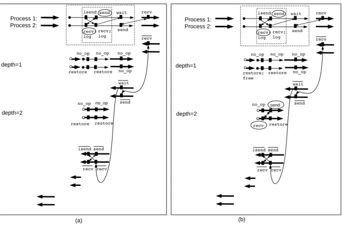
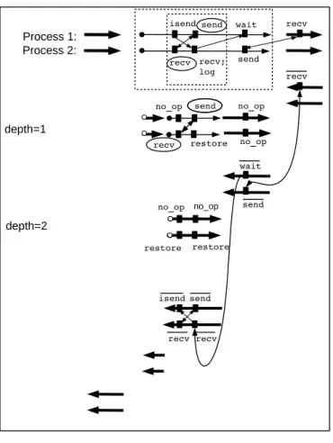
isend send wait recv recv; log send recv; log send no_op no_op restore restore no_op no_op restore wait recv no_op no_op send recv recv isend Process 1: Process 2: depth=1 depth=2
isend send wait recv
recv; log send recv; log send no_op no_op restore restore; free no_op send recv restore wait recv no_op no_op send recv recv isend Process 1: Process 2: depth=1 depth=2 restore (a) (b)
Figure 6: (a) Checkpointing a parallel adjoint program on two nested checkpointed parts by using the receive-logging method. (b) Refinement of the checkpointed code by applying the message re-sending to a send-recv pair with respect to the inner checkpointed code which is right-tight
Figure 6 (a) shows the example of two nested checkpointed parts together with an arbitrary communication pattern that straddles across the boundaries of the checkpointed parts.
During execution of the duplicated checkpointed parts, no communication call is made and receive operations read from the local storage instead. We can see that the communication pattern of the forward sweep is preserved by checkpointing, the communication pattern of the backward sweep is also preserved, and no communication takes place during duplicated parts.
To show that this strategy is correct, we will check that it verifies the two assumptions of section 2.
3.1 Correctness
By construction, this strategy respects Assumption 1 because the duplicated receives read what the initial receives have received and stored.
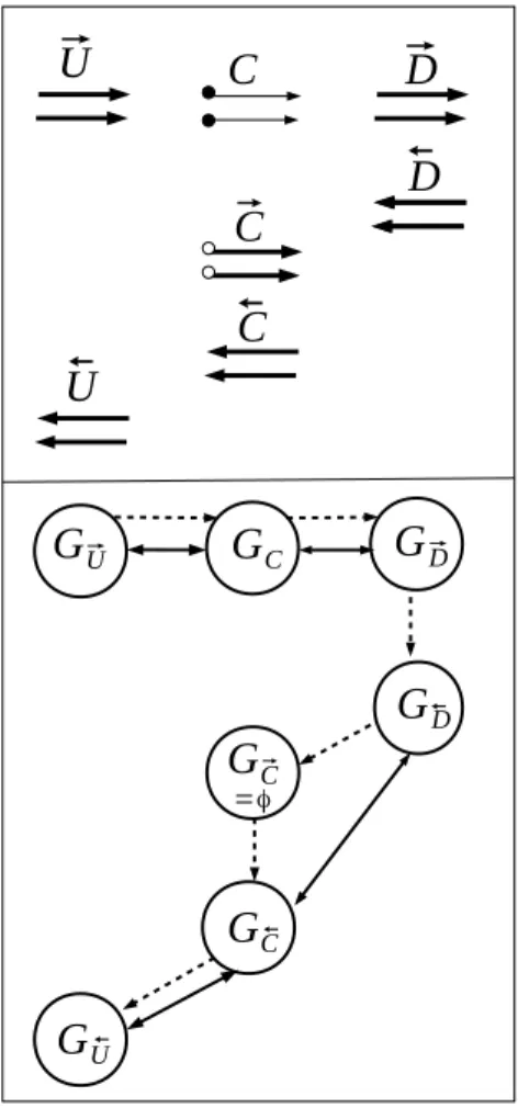
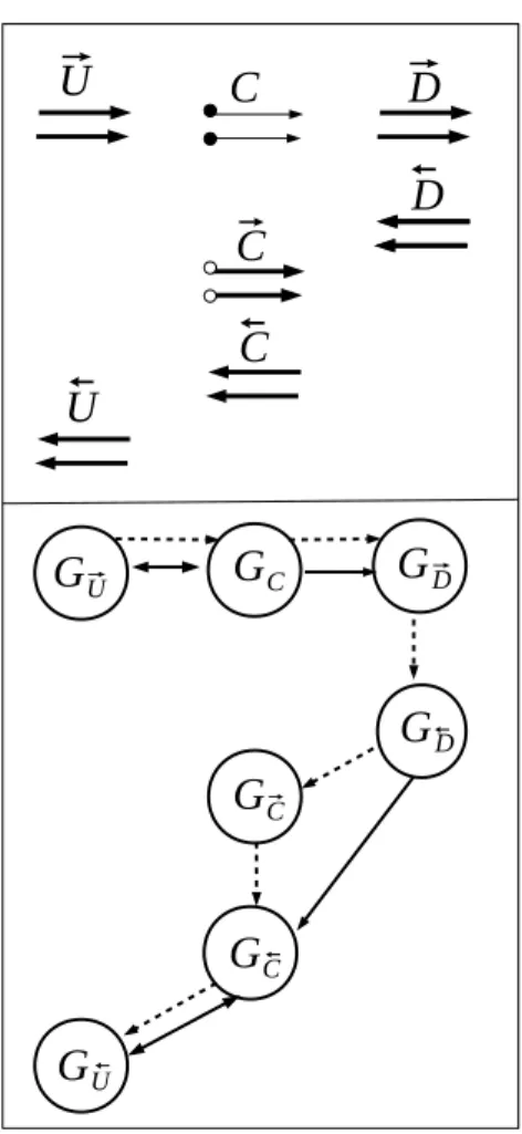
To verify Assumption 2 about the absence of deadlocks, it suffices to consider one elementary application of checkpointing, shown in the top part of figure 7. Communications in the check-pointed code occur only in −→U , −→C , −→D (about primal values) on one hand, and in ←D ,− ←C ,− ←U− (about derivatives) on the other hand. The bottom part of the figure 7 shows the communica-tions graph of the checkpointed code, identifying the sub-graphs of each piece of code. Dotted arrows express execution order, and solid arrows express communication dependency. Com-munications may be arbitrary between G−→
U, GC and G−→D but the union of these 3 graphs is the same as for the forward sweep of the non-checkpointed code, so it is acyclic by hypothesis. Similarly, communications may be arbitrary between G←−
def-G
⃗UG
CG
⃗DG
DG
CG
U ⃗G
⃗C⃗
U
⃗
D
⃗
C
U
D
C
⃗
⃗
⃗
C
=φ ⃗ ⃗Figure 7: Communications graph of a checkpointed program with pure receive-logging method
inition empty) these graphs are the same as for the non-checkpointed backward sweep. Since we assume that the non-checkpointed code is deadlock free, it follows that the checkpointed code is also deadlock free.
3.2 Discussion
The receive-logging strategy applies for any choice of the checkpointed piece(s). However, it may have a large overhead in memory. At the end of the general forward sweep of the complete program, for every checkpointed part (of level zero) encountered, we have stored all received values, and none of these values has been used and released yet. This is clearly impractical for large codes.
On the other hand, for checkpointed parts deeply nested, the receive-logging has an acceptable cost as stored values are used quickly and their storage space may be released and used by checkpointed parts to come. We need to come up with a strategy that combines the generality of receive-logging with the memory efficiency of an approach based on re-sending.
4 USING MESSAGE RE-SENDING WHENEVER POSSIBLE
We may refine the receive-logging by re-executing communications when possible. The principle is to identify send-recv pairs whose ends belong to the same checkpointed part, and to re-execute these communication pairs identically during the duplicated part, thus performing the actual communication twice. Meanwhile, communications with one end not belonging to
the checkpointed part are still treated by receive-logging.
However, the checkpointed part must obey an extra constraint which we will call “right-tight”. A checkpointed part is “right-tight” if no communication dependency goes from down-stream the checkpointed part back to the checkpointed part, i.e. there is no communication dependency arrow going from D to C in the communications graph of the checkpointed code. For instance, there must no wait in the checkpointed part that corresponds with communica-tion call in other process which is downstream (i.e. after) the checkpointed part.
Figure 6 (a) shows an example of two nested checkpointed parts in which the outer check-pointed part is not right-tight, whereas the inner checkcheck-pointed part is right-tight since the de-pendency from the second recv of process 2 to the wait of the isend of process 1 only goes from the checkpoint inside to its outside. In the figure 6 (a), we identify a send-recv pair (whose ends are surrounded by circles) that belongs to both nested checkpointed parts. As the outer checkpointed part is not right-tight, we can apply the message re-sending to the send-recvpair only with respect to the inner checkpointed part. We see on figure 6 (b) that the send-recv pair is re-executed during the execution of the duplicated instance of the inner checkpointed part. As the duplication of the pair send-recv is placed between the wait of process 1 and the first recv of process 2 and since wait is a non blocking routine, the duplication of this send-recv pair does not create deadlock in the resulting adjoint.
isend send wait recv recv; log send recv send no_op send restore recv no_op no_op restore wait recv no_op no_op send recv recv isend Process 1: Process 2: depth=1 depth=2 restore
Figure 8: Application of the message re-sending to a send-recv pair with respect to the outer checkpointed part which is not right-tight
to a checkpointed part which is not right-tight. We reuse the example of figure 6 (a). Instead of applying the message re-sending to the pair send-recv (whose ends are surrounded by circles) with respect to the inner checkpointed code as it is the case in figure 6 (b), we applied the message re-sending to the pair send-recv with respect to the outer checkpointed code which is not right-tight. Figure 8 shows the cycle in the communications graph of the resulting adjoint. We see on the figure that, between the recv of process 1 and the send of process 2 takes place the duplicated run of the outer checkpointed part. In this duplicated run, we find a duplicated send-recv pair that causes a synchronization. Execution thus reaches a deadlock, with process 1 blocked on the recv, and process 2 blocked on the duplicated recv.
Only when the checkpointed part is right-tight can we mix message re-sending of communi-cations pairs that are contained in the checkpointed part with receive-logging of the others. The interest is that memory consumption is limited to the (possibly few) logged receives. The cost of extra communications is tolerable compared to the gain in memory.
4.1 Correctness
G
⃗UG
CG
⃗DG
DG
CG
UG
⃗C⃗
U
⃗
D
⃗
C
U
D
C
⃗
⃗
⃗
C
⃗ ⃗ ⃗Figure 9: Communications graph of a checkpointed program by using the receive-logging coupled with the mes-sage re-sending
The subset of the duplicated receives that are treated by receive-logging still receive the same value by construction. Concerning the duplicated send-recv pair, the duplicated check-pointed part computes the same values as its original execution (see step from σ05to σ60 in section 2 ). Therefore the duplicated send and the duplicated recv transfer the same value.
The proof about the absence of deadlocks is illustrated in figure 9. In contrast with the pure receive-logging case, G−→
C is not empty any more because of re-sent communications. G−→C is a subgraph of GC and is therefore acyclic. Since the checkpointed part is right-tight, the depen-dency from GC to G−→
D and from G←D−to G←C− are unidirectional. There is no communication dependency between G−→
C and G←D− and G←C− because G−→C communicates only primal values and G←−
D an G←C−communicate only derivative values.
Assuming that the communications graph of the non-checkpointed code is acyclic, it follows that:
• Each of G−→
U, G−→C, G−→D, G←D−, G←C− and G←U−is acyclic. • Communications may be arbitrary between G−→
U and GC but since these pieces of code occur in the same order in the non-checkpointed code, and it is acyclic, there is no cycle involved in (G−→
U; GC). The same argument applies to (G←C−; G←U−). Therefore, the complete graph on the bottom of figure 9 is acyclic.
5 DISCUSSION AND FURTHER WORK
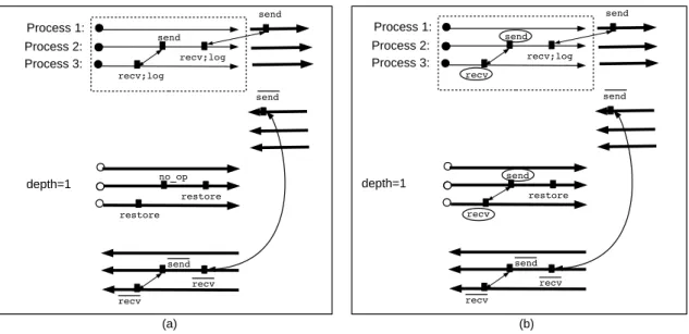
Process 1: send send Process 2: recv;log recv;log depth=1 Process 3: (a) (b) send no_op restore restore send recv recv Process 1: send send Process 2: recv;log recv depth=1 Process 3: send send restore recv send recv recv
Figure 10: (a) The receive-logging applied to a parallel adjoint program. (b) Application of the message re-sending to a send-recv pair with respect to a non-right-tight checkpointed code
We studied checkpointing in the case of MPI parallel programs with point-to-point com-munications. We proved that any technique that adapts the checkpointing mechanism to MPI parallel programs and that respects some sufficient conditions, is a correct MPI checkpointing technique, in the sense that, the checkpointed code resulting from the application of this MPI checkpointing technique preserves the semantics of the non-checkpointed adjoint code. We introduced, a general MPI checkpointing technique that respects the sufficient conditions for any choice of the checkpointed part. This technique is based on logging the received messages , so that the duplicated communications need not take place. We proposed a refinement that reduces the memory consumption of this general technique by duplicating the communications whenever possible. There are a number of questions that should be studied further:
We imposed a number of restrictions on the checkpointed part in order to apply the refine-ment. These are sufficient conditions, but it seems they are not completely necessary. Figure 10 shows a checkpointed code which is not right-tight. Still, the application of the message re-sending to a send-recv pair (whose ends are surrounded by circles) in this checkpointed part, does not introduce deadlocks in the resulting checkpointed code.
In real codes we may have nested structure of checkpointed parts in which each checkpointed part may be or not right-tight. Applying the message re-sending to only checkpointed parts that are right-tight means that some communication calls will be activated in some levels and deactivated in the other levels. Thus, to implement the refined receive-logging, we need to think about the way we could automatically alternate between these two situations for each communication call. For instance, a receive that is deactivated at a level and activated at the level just after has to release its stored value.
Finally, these checkpointing techniques need to be experimented in real codes. It would be interesting to measure the memory consumption of the general checkpointing technique before and after the application of message re-sending.
6 ACKNOWLEDGEMENT
This research is supported by the project “About Flow”, funded by the European Commission under FP7-PEOPLE-2012-ITN-317006. See “http://aboutflow.sems.qmul.ac.uk”.
REFERENCES
[1] A. Griewank, A. Walther, Evaluating Derivatives: Principles and Techniques of Algorith-mic Differentiation. Other Titles in Applied Mathematics, #105. SIAM, 2008.
[2] M. Snir, S. Otto, The Complete Reference: The MPI Core. Cambridge, MA, USA: MIT Press, 1998.
[3] P. Hovland, Automatic differentiation of parallel programs Ph.D. dissertation, University of Illinois at Urbana-Champaign, 1997.
[4] A. Carle, M. Fagan, Automatically differentiating MPI-1 datatypes: The complete story, in Automatic Differentiation of Algorithms: From Simulation to Optimization, ser. Computer and Information Science, G. Corliss, C. Faure, A. Griewank, L. Hasco¨et, and U. Naumann, Eds. New York: Springer, 2002, ch. 25, pp. 215-222.
[5] P. Heimbach, C. Hill, R. Giering, An efficient exact adjoint of the parallel MIT general circulation model, generated via automatic differentiation Future Generation Computer Systems 21. 2005. p. 1356-1371.
[6] U. Naumann, L. Hasco¨et, C. Hill, P. Hovland, J. Riehme, J. Utke, A Framework for Prov-ing Correctness of Adjoint Message PassProv-ing Programs. In Recent Advances in Parallel Virtual Machine and Message Passing Interface. Springer. 2008. p. 316-321.
[7] J. Utke, L. Hasco¨et, P. Heimbach, C. Hill, P. Hovland, U. Naumann, Toward Adjoinable MPI. Proceedings of the 10th IEEE International Workshop on Parallel and Distributed Scientific and Engineering, PDSEC’09, 2009.
[8] B. Dauvergne, L. Hasco¨et, The Data-Flow Equations of Checkpointing in reverse Au-tomatic Differentiation. International Conference on Computational Science, ICCS 2006, Reading, UK, 2006.
[9] F. Capello, A. Geist, W. Gropp, S. Kale, B. Kramer, M. Snir, Toward Exascale Resilience: A 2014 Update. Supercomput.Front. Innovations 1(1) (2014).