Publisher’s version / Version de l'éditeur:
Vous avez des questions? Nous pouvons vous aider. Pour communiquer directement avec un auteur, consultez la première page de la revue dans laquelle son article a été publié afin de trouver ses coordonnées. Si vous n’arrivez pas à les repérer, communiquez avec nous à [email protected].
Questions? Contact the NRC Publications Archive team at
[email protected]. If you wish to email the authors directly, please see the first page of the publication for their contact information.
https://publications-cnrc.canada.ca/fra/droits
L’accès à ce site Web et l’utilisation de son contenu sont assujettis aux conditions présentées dans le site LISEZ CES CONDITIONS ATTENTIVEMENT AVANT D’UTILISER CE SITE WEB.
Internal Report (National Research Council of Canada. Institute for Research in Construction), 1995-11-01
READ THESE TERMS AND CONDITIONS CAREFULLY BEFORE USING THIS WEBSITE. https://nrc-publications.canada.ca/eng/copyright
NRC Publications Archive Record / Notice des Archives des publications du CNRC :
https://nrc-publications.canada.ca/eng/view/object/?id=11d7cf0f-21d9-42c2-9b49-5096844e8022 https://publications-cnrc.canada.ca/fra/voir/objet/?id=11d7cf0f-21d9-42c2-9b49-5096844e8022
NRC Publications Archive
Archives des publications du CNRC
For the publisher’s version, please access the DOI link below./ Pour consulter la version de l’éditeur, utilisez le lien DOI ci-dessous.
https://doi.org/10.4224/20375335
Access and use of this website and the material on it are subject to the Terms and Conditions set forth at Field Study of Office Thermal Comfort Using Questionnaire Software
A Field Study of Office Thermnl Comfort Newsham & Tiller 3
Abstract
ScreenSurvey, custom software to automatically administer questionnaires on computer
screens, was installed on the computers in open-plan office spaces at four sites. Five questions related to thermal comfort were presented twice per day for three months; internal and external climate data were collected simultaneously. Data from a 10 week period were recovered from 55 participants. Results indicate that this new method of subjective data collection was successful and efficient: the participants had few complaints about the method of questionnaire delivery; and a substantial literature review
demonstrates that the results of our study are comparable with results from other field studies of thermal comfort conducted using different methods. Participants responded to the auestionnaire 29 % of the occasions on which it could have been ~resented, and took an average of 45 seconds to answer the five questions. 87 % of votes were in the central three categories ('slightly cool' to 'slightly warm') of the ASHRAE thermal sensation scale, and 70 % of thermal preference votes indicated a desire for no change in temperature; we derived a neutral temperature of 22.7 O C . Overall, the number of thermal sensation votes indicating thermal acceptability was as predicted by
ANSIIASHRAE Standard, and by the comfort theory on which this Standard was based. However, our results indicate a greater sensitivity to temperatures away from the neutral temperature than theory predicts. Only 11 % of the variance in thermal sensation vote was explained by indoor air temperature, which rose to only 14 % when other measured physical and personal parameters were included in the regression. Differences in thermal sensation vote by age, sex, or office orientation were either not significant, or small. There were no significant differences in thermal sensation vote by week or hour, though the small changes in mean vote were in the expected direction. Around 15 % of people changed their clothing in the hour prior to the questionnaire appearing, suggesting that clothing change may be an important mechanism for achieving thermal comfort.
A Field Study of Office Thermal Comfort Newsham & Tiller 4 Contents ACKNOWLEDGMENTS
...
2...
ABSTRACT 3...
CONTENTS 4 1.0 INTRODUCTION...
6 1.1 BACKGROUND ... 61.2 A BRIEF SUMMARY OF THERMAL COMFORT RESEARCH ... 6
... 1.3 TRANSIENT CONDITIONS AND THE NEED FOR LONGITUDINAL STUDIES 8
...
2.0 MATERIALS AND METHODS 9...
2.1 PERIOD OF STUDY 9 2.2 STUDY SITES ... 9 2.3 PARTICIPANTS ... 2.4 MEASUREMENT OF OUTDOOR C ... 2.5 MEASUREMENT OF INDOOR CLIMATE 11 2.6 RECORDING PARTICIPANTS' REACTIONS AND PERSONAL INFORMATION ... 12... 2.7 FINAL EVALUATION QUESTIONNAIRE 13 3.0 RESULTS
...
143.1 OUTDOOR CLIMATE vs
.
TIME...
....
3.2 INDOOR CLIMATE vs TIME ... 3.3 RESPONSERATE AND RESPONSE TlME 14 ... 3.4 AGGREGATE FREQUENCY DATA 14 3.5 ORDER EFFECT ... 17...
3.6 CORRELATIONS BETWEEN DATA 18 3.7 REGRESSIONS BETWEEN PARTICIPANT RESPONSES AND PHYSICAL MEASURES ... 183.8 THE EFFECT OF RESPONSE RATE ON REGRESSIONS
...
203.9 NEUTRAL AND PREFERRED TEMPERATURES ... 21
... 3.10 COMPARISON WITH PREDICTED MEAN VOTE (PMV) 3.1 1 DIFFERENCES BETWEEN 3.12 LONGITUDINAL DATA
...
3.13 ANALYSIS OF FINAL EVALUATION QUESTIONNAIRE 4.0 DISCUSSION...
284.1 FREQUENCY OF RESPONSE ... 28
... 4.2 COMPARISON OF FREQUENCY DATA WITH THERMAL COMFORT STANDARDS 29 4.3 CORRELATIONS BETWEEN PARAMETERS
...
314.4 EFFECT OF RESPONSE RATE ... 1
4.5 OVERALL SATISFACTION
...
.
.
...
24.6 REGRESSING THERMAL SENSATION ON TEMPERATUR 3 4.7 DESIRABILITY OF THERMAL NEUTRALITY ... ... 9
...
... 4.8 COMPARISON WITH PMV.
.
94.9 CLOTHING AND CLOTHING MOD~CATION 1 4.10 LONGITUDINAL DATA ... 43
4.1 1 OTHER DEMOGRAPHIC GROUPINGS DATA ... 45
4.12 RNAL EVALUATION QUESTIONNAIRE
...
47-0rt Newshorn & Tiller 5
...
5.0 CONCLUSIONS 49 ... 5.1 SUCCESS OF METHOD 49 ... 5.2 A~CREOAEFI~EQIENCY DATA 495.3 THERMAL SENSATION CORRELAIIONS AND REGRESSIONS
...
0...
...
5.4 NEUTRAL AND PREFERRED TEMPERATURES.
.
.
1...
5.5 COMPARISON WITH PMV 51...
5.6 DIFFERENCES BETWEEN DEMOGRAPHIC GROUPINGS 51...
5.7 LONGITUDINAL RES~NSEJCOMFORT DATA 52 5.8 COMPARISON OF FREQUENCY DATA WITH THERMAL COMFORT STANDARDS ... 525.9 SCREENSURVEY DEVELOPM ENT. ... 53
6.0 REFERENCES
...
54 FIGURES...
61 APPENDICES...
%...
APPENDIX A 97 APPENDIX B...
110 APPENDIX C...
113 APPENDIX D...
114A Field Study of Office nermal Comfon Newsham & Tiller 6
1.0 Introduction 1.1 Background
Longitudinal studies of subjective reactions can be very useful in identifying problems with the indoor environment, particularly those that change over time. Comparing subjective reactions with the prevailing physical aspects of the indoor environment can help identify the sources of problems, which facilitates solving the problems.
While the physical aspects of the indoor environment can be easily measured over time using automatic data logging technology, measuring the concurrent subjective reactions is
difficult. The traditional method of obtaining subjective reactions data is the paper questionnaire. However, using paper questionnaires to perform longitudinal surveys -- which requires administering the same questionnaire many times
--
would be d i s ~ p t i v e , expensive, and labour intensive.To overcome these problems, the National Research Council of Canada
(NRC)
has developed custom software, called ScreenSurvey, to automatically administerquestionnaires on computer users' screens at dates and times specified by the experimenter in a data file. The software is described in more detail in Section 2.6.
This study had two aims:
1. To test ScreenSurwey's usefulness as a tool for gathering longitudinal subjective reactions data in the field.
2. To use the field test data to study the relationship between the thermal environment in open-plan office spaces and the thermal comfort of its occupants.
1.2 A Brief Summary of Thermal Comfort Research
In post-occupancy studies, the thermal environment is frequently rated as one of the most important aspects of a healthy, pleasing, and productive workplace [Baillie et. al, 1988; de Dear et al., 1993; Jaakkola et al,, 1989; Rohles et al., 19891. Many studies have been performed to try to elucidate the relationship between human thermal sensation and the physical environment. The principal goal of this research is to determine what physical parameters are conducive to a comfortable, and productive' indoor environment, and how best to deliver those physical parameters. Research has focused on the physical
parameters (rather than on psychological parameters, for example) because, in practice, these are the parameters that designers and building managers can directly influence.
1
Research attempting to link productivity, learning and related factors to the thermal environment in various settings has been extensive. The results are varied and remain largely inconclusive. See, for example: AUen & Fischer [19781, Howell & Kennedy [1979], Langkilde et al. [1973], Lorsch & Abdou
A Field Study of Office Thermal Comfort Newsham & Tiller 7
The research falls into two camos: laboratorv studies, and field studies. In laboraton, studies, participants typically siiin climate chambers wearing fixed standardized clo&ing ensembles and remain sedentary while experiencing thermal environments chosen by the experimenters, or adjusting the thermal environment (normally air temperature) themselves in order to achieve an optimum environment Most codes and standards are based on laboratory studies of this type, particularly the seminal work of Fanger [1970]. Fanger found that in climate chamber studies the mean reported thermal sensation of a group of people exposed to the same thermal environment was a function of four physical
parameters
(air
temperature, mean radiant temperature, humidity, air speed), and two personal parameters (clothing, metabolic rate).While the laboratory affords the usual advantages of being able to manipulate and measure the stimuli exactly, there have been numerous criticisms of laboratory studies of thermal comfort. The criticisms can generally be grouped under the heading of external validity, that is, how well do the results translate to the real world where they will be applied. Firstly, the climate chambers tend to be stark, sterile spaces, not aesthetically similar to most real world interiors. Secondly, the participants do not perform tasks representative of real world tasks. Thirdly, manv of the oarameters held constant in laboratory studies are not constant in the realhodd:~clothing. for example. Fourthly, the participants in laboratory studies are usually college students, not very representative of the real world population.
In field studies, participants typically report their thermal sensations in situ while all
important parameters are recorded at their prevailing values. The results are usually compared to the predictions made from the results of laboratory studies in order to test the &idity of the laboratory studies; in many cases, the data coilected in field studies have proven incompatible with the laboratory studies. However, these comparisons are
complicated by the difficulty of precisely defining the relevant parameters in the field. For example, in the context of Fanger's equation, accurately determining an individual's clothinrr insulation and metabolic rate in a oractical manner in the field is extremely difficuc. Baker and Standeven [I9951
arGe
that Fanger's physics and physiolog; are correct, and that field and laboratory measurements are perfectly consistent. Differences are due to uncertainty in physical &d personal due to measurement errors or behavioral adjustments made by occupants, resulting in local thermal conditions that differ from those at measurement points and from assumptions. However, Oseland [I9941 found that the same participants in similar clothing and thermal environments felt warmest in their homes, next warmest in their office, and coolest in climate chambers. Oseland argues that this finding points to a genuine context effect that goes beyond physics and physiology. There has been a considerable and on-going effort to conduct field studies on many different populations in many different geographical locations. The data collected in our study add to this body of work, and comparisons to prior research, particularly to other field studies, will be made throughout this report.A Field Study of Oflice Thermal Comfon Newsham & Tiller 8
1.3 Transient Conditions and the Need for Longitudinal Studies
The vast majority of laboratory studies have examined thermal comfort under fiied thermal conditions. Those laboratory studies that have looked at transient conditions m c e l l & Thome, 19871 have done so in a very mechanistic way, with the changes being provided by a climate control system invisible to the participants, and according to regular mathematical functions. Baillie et al. 119881, Hensen [1990], and Oseland & Humphreys [I9931 called for an investigation of the effect of more realistic changes in the thermal environment, such as those caused by solar radiation, or by moving between different spaces. Indeed, Black & Milroy [I9661 observed in a field study that overheating was reported not on a regular schedule, but at times of day when the sun was shining. The only way to capture this kind of information in a field study is to conduct a
longitudinal (or time-series) study; that is,
a
study in which opinions (in this case, thermal sensation votes) are surveyed many times over the study period. In this way, theinvestigator can: observe how participants' reactions change in response to a changing physical environment; observe how past experience influences reactions; avoid the possibility that a snapshot survey captured atypical information [Cena et al., 1990; Humphreys, 1994; Nicol & Humphreys, 19731. Longitudinal data could also be used to establish behaviour patterns
as
input to an adaptive model of thermal comfort which would take into account people's ability to temper their environment through personal or physical changes [Baker & Standeven, 1985; de Dear 1994; Hensen 1990; Humpbreys & Nicol, 1970; Humphreys, 1994; Paciuk, 19891As noted in Section 1.1, conducting longitudinal surveys in the field using paper questionnaires would be disruptive, expensive, and labour intensive. Recognizing this,
Humphreys & Nicol [I9701 and Fishman & Pimbert [I9821 conducted longitudinal studies in the field using voting box hardware to collect thermal sensation votes automatically. Each participant in each study had a box about the size of a telephone placed on their desk. At regular intervals the box cued the participant to vote using an audible tone. The participant voted by pressing one of seven buttons on the box, each button corresponding to a response on a thermal comfort scale. Sensors attached to the box simultaneously recorded various physical parameters of the thermal environment These systems worked reliably, collecting much valuable data. However, the number of participants was limited (presumably by the cost of manufacturing the boxes), and the number and variety of responses were limited by the arrangement of buttons on the box. With ScreenSurvey we hoped to build on the success of these longitudinal studies. Embodiment of the voting box principal in software provided a great deal more flexibility in the number of questions asked and the variety of responses offered, and allowed us to increase the number of participants, because the cost of reproducing software is negligible.
A Field Study of Office Thermal Comfort Newsham & Tiller 9
2.0 Materials and Methods 2.1 Period of Study
Data collection took place during the period October, 1994 to January, 1995, or late Fall and early Winter.
2.2 Study Sites
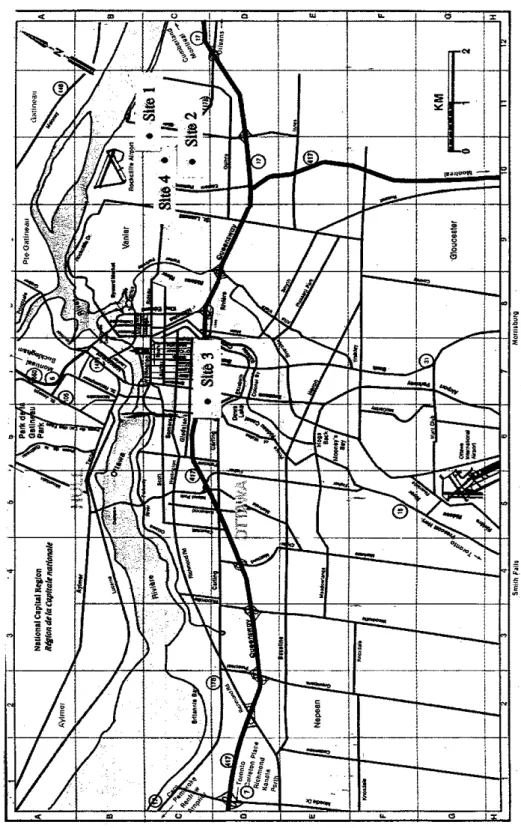
The study was carried out at four sites. All sites were federal government facilities in Ottawa, Ontario, Canada. Figure 1 shows general outdoor climate data for this region. Ottawa is located at latitude 45O 19' N, longitude 7.5' 40' W (see Figure 2). Figure 3 is a street map of Ottawa showing the locations of the four sites within the city.
2.2.1 Site I
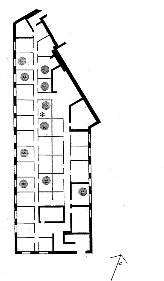
Site 1 was an open-plan office occupying part of the second floor of a three storey
suburban building. The occupants of this site did facilities design work. Figure 4 is a floor plan of the site, indicating the positions of the study participants. 5 illustrates the appearance of the site.
2.2.2 Site 2
Site 2 was an open-plan office occupying part of the first floor of a seven storey suburban building. The occupants of this site did a variety of bibliographic tasks. Figure 6 is a floor plan of the site, indicating the positions of the study participants. Figure 7 illustrates the appearance of the site.
2.2.3 Site 3
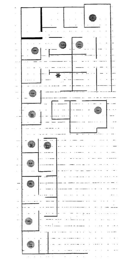
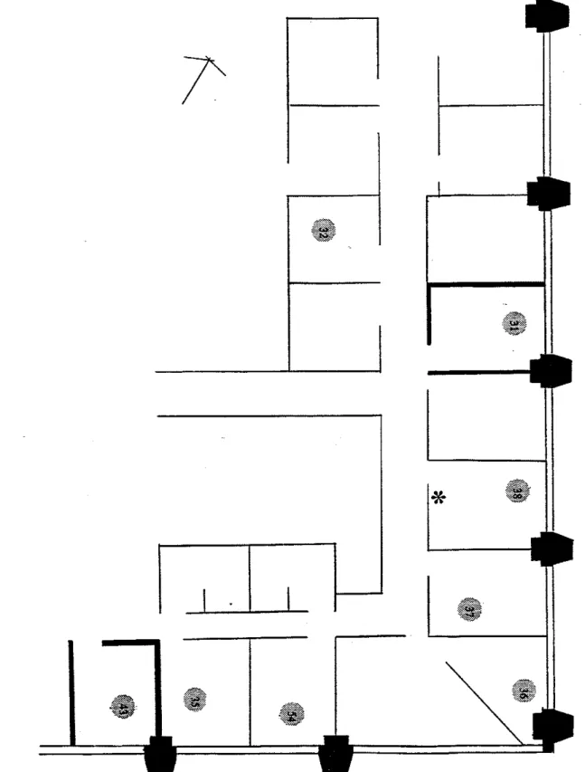
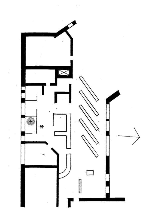
Site 3 was a mostly open-plan office occupying the whole of the seventh floor, and part of the ninth floor, of a twenty-four storey downtown building. The occupants of this site did a variety of administrative, technical and scientific tasks. Figures 8(a) and 8(b) are floor plans of the site, indicating the positions of the study participants. Figure 9 illustrates the appearance of the site.
2.2.4 Site 4
Site 4 was an open-plan office occupying part of the second floor of a three storey suburban building. The occupants of this site did a variety of bibliographic tasks. Figure
10 is a floor plan of the site, indicating the positions of the study participants. Figure 11 illustrates the appearance of the site.
A Field Study of Office Thermal Comfort Newsham & Tiller 10
2.3 Participants
After receiving approval from NRC's Human Subjects Research Ethics Committee
(HSREC) for the study, we asked the managers at various sites for permission to approach their staff and to invite them to volunteer for the study. Managers at the four sites
described in Section 2.2 agreed to this. At each site we met with each staff member face- to-face, explained the project to them and invited them to participate. Those who agreed to participate were asked to sign a consent form (shown in Appendix A), and were given some written information on the project (see Appendix A). They were told that the
software would be installed on their computer within a week, and that it would be installed outside of normal working hours. When we installed the software we left each participant written information on each of the questions that would be asked (see Appendix A). The software was installed on over 60 comouters at the four sites. At the conclusion of the study period, useful data were recovered from 55 participants. Of these 55
participants, 50 returned the basic demographic information shown in Table 1.
Table I . Participant demographic information.
Sex
Age Female Male
X
20 - 29 8 1 9 30 - 39 5 13 18 40
-
49 7 11 18 50 - 59 1 3 4 60 - 69 0 1 1C
2 1 29 50AU
written information was supplied in either English or French, according to the participant's preference. In addition, the on-screen questionnaire was delivered in the language of the participant's preference. Table 2 shows the language of preference of the 55 participants from whom useful data were collected.Table 2. Participant language of preference.
Language of Preference
French English C
7 48 55
2.4 Measurement of Outdoor Climate
Outdoor climate data were recorded at an electronic weather station located close to site 4. The data recorded at this station were used for all sites, though some local differences may have occurred.
A Field Study of Office Thermal Comfort Newsham & Tiller I I
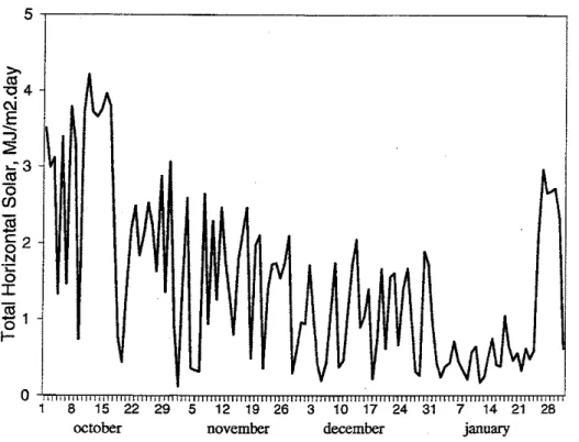
The weather station recorded many climate parameters. The parameters of interest to this study were: mean relative humidity, mean air temperature, and total solar radiation on a horizontal plane. Each of these parameters was recorded hourly during the study period. The weather data were recorded by a Sciemetrics 200 Data Acquisition System. The raw data was stored in ASCII format, and were made available on the local computer network at the end of each month.
Total solar radiation on a horizontal plane was converted to total solar radiation on a vertical plane in each of the four cardinal directions using correlation equations [Barakat, 1983; Orgdl& Hollands, 19771.
2.5 Measurement of Indoor Climate
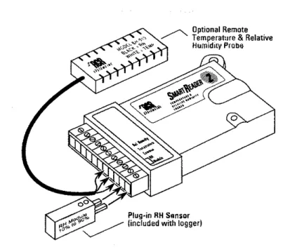
Indoor air temperature and relative humidity were measured at the four sites using ACR Smartreader 2 dataloggers (shown in Figure 12). These dataloggers have a local capacity of 32,000 readings; these data were downloaded into a personal computer for analysis. Climate chamber tests confmed the factory calibration and claimed accuracy of the loggers' sensors, as shown in Table 3.
Table 3. Accuracy of the indoor climate sensors.
Sensor Accuracy
Air temperature j, 0.4 "C
Relative Humidity f 4 %
Ideally, physical measures would have been taken at each of the participants'
workstations. However, only a limited number of dataloggers were available. Therefore, we placed the loggers at representative points at the four sites (shown in Figures 4,6,8, and 10). Sites 1,2,4, and the ninth floor of site 3, where the office spaces were
predominantly on a single facade, received one logger each. Five loggers were placed on the seventh floor of site 3, where there were offices on four facades and in a core area. Care was taken not to place the loggers in unrepresentative locations, such as: places where they would receive direct sunlight, and places close to sources of internal heat gain. The loggers are small (107 x 74
x
22 mm) and highly portable, and were secured to office furniture using 3/32)) steel cable.The dataloggers were programmed to record both indoor air temperature and relative humidity every 20 minutes for the duration of the study period. About two weeks after installing the dataloggers, we returned to check that they working correctly. After that, we did not visit them again until the end of the study period, when the data were
A Field Study of Ofice 17lermal Comfort Newshom & Tiller 12
2.6 Recording Participants' Reactions and Personal Information 2.6.1 ScreenSurvey Sojiware
Subjective reactions to the indoor thermal environment were collected using NRC's
ScreenSurvey software. This study was carried out using version 1 of the software, and it
is version 1 that is described here. NRC has since developed version 2 of the software, which has enhanced capabilities (described briefly in Section 5.9).
ScreenSurvey automatically administers questionnaires on computer users' screens. When
administered, the questionnaire takes the form of a "window" over the user's other open applications. The individual questions are designed using custom Form Builder software. The questions have one of three response types:
1. A list of responses from which the participant may pick only one;
2. A list of responses from which the participant may pick as many as apply;
3. A sliding scale labeled with descriptors: the participant places
a
pointer on the scale at a position which best describes their response.Once created, the questions can then be administered in any order, at dates and times specified by the experimenter in
a
data file. Any number of questions may be asked with any frequency. The questions are always preceded by a "Warning Banner", that asks the participant if they would like to continue with the questionnaire (see Figure 13). If the participant clicks "Cancel", or if there is no reply after a given time period, then the questionnaire can be rescheduled. In addition, certain questions can be defined as "demographic" questions, which are asked only once; these are questions for which the answers would not be expected to change over time. The responses to the questions are stored on the host computer's hard disk for collection at the end of the study by the experimenter.ScreenSurvey was available for both Macintoshm and windowsm operating systems.
Table 4 shows the number of each type of computer operating system used by the participants.
Table 4. Operating system of Participants' computers.
Operating System
Macintoshm ~ i n d o w s ~ Z
2.6.2 Questions Asked
The questions asked were divided into two types: demographic questions, and recurring questions.
A Field Study of Ofice n t e r m l Comfon Newshnm & Tiller 13
Demographic questions are asked only once because answers are not expected to change with time (e.g., sex, mother tongue). The demographic questions were asked within one minute of the participant switching their computer on following installation of the
ScreenSurvey software.
Recurring questions are questions that are asked many times; they are questions to which the answer would be expected to change with time. Recurring questions were asked twice per day, once before 1300 hrs and once after 1300 hrs, for the duration of the study. The times at which the questions appeared, and the order in which they appeared followed a pseudo-random but pre-defined schedule, described in Appendix B. Each participant followed the same schedule. Appendix A shows the four demographic and five recuning questions asked.
2.7 Final Evaluation Questionnaire
When we returned at the end of the study period to remove ScreenSurvey from
participants' computers and collect the recorded data, we left behind a paper-based, final evaluation questionnaire. The purpose of the questionnaire was to evaluate the
performance of ScreenSurvey and tn invite any suggestions for improvements. We anticipated that suggested improvements would be taken into consideration when upgrading ScreenSurvey. Appendix C shows the content of the final evaluation questionnaire.
Participants returned the completed final evaluation questionnaire via normal internal mail channels.
A Field Study of Office Thermal Comfort Newshnm & Tiller I4
3.0 Results
Results are presented in this section with minimal accompanying comments. Detailed discussion of results is reserved for Section 4. Participant data collected using
ScreenSurvey is presented for the 10 week period: October 15th. 1994 to December 23rd,
1994.
3.1 Outdoor Climate vs. time
Figure 14(a) shows the outdoor air temperature recorded at the weather station during the period of the study. Figures 14(b) and 14(c) show similar plots for relative humidity and total solar radiation respectively. The thick lines show the mean values for each day; for air temperature and relative humidity the "whiskers" show the maximum and minimum values for each day.
3.2 Indoor Climate vs. time
Figure 15 plots indoor air temperature and relative humidity at Site 1 for during the period 21st - 27th November, 1994. These data represent a typical week's readings, and
illustrates the typical within-day and between-day variations that occurred at the sites. 3.3 Response Rate and Response Time
Each recurring question could have been answered a maximum of 100 times over the 10 week period. The mean response rate to the ASHRAE thermal sensation question
(Appendix A) was 29.1 % (n = SS), s.d. = 12.7., which represents 1600 data points. In other words, each participant answered the ASHRAE thermal sensation question an average of 29 times during the ten week period (the response rate to other questions differed, response rates to each question are discussed later). Figure 16 shows the actual response rate of each participant. The minimum response rate was 2 %, the maximum response rate was 62 %.
When participants responded, it took an average of 45.3 s (n = 1600), s.d. = 32.6 to answer all five questions. Figure 17 shows the mean response time of each participant The minimum mean response time was 29.6 s, the maximum mean response time was
100.7 s.
3.4 Aggregate Frequency Data
In this section, the data from all sites and participants has been grouped.
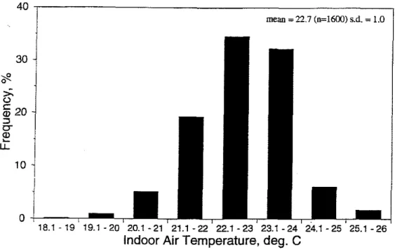
Figure 18 shows the frequency of indoor air temperature prevailing when the participants responded to the ScreenSurvey questionnaire (to at least the ASHRAE thermal sensation . .
question). For Figure 18, the air temperatures were sorted into 1 O C bins. Remember,
A Field Study of Office Thermal Comfon Newsham & Tiller IS
ScreenSurvey. Therefore, in this context, 'prevailing when the participant responded to
the ScreenSurvey questionnaire' means: recorded within 20 minutes of the time when the participant responded to the ScreenSurvey questionnaire. The mean indoor air
temperature was 22.7 OC (n = 1600), s.d. = 1.0. The modal indoor air temperature was 22.1
-
23.0 OC, this bin represented 34.6 % of the recorded temperatures.Figure 19 shows similar frequency information for the indoor relative humidity prevailing when the participant responded to the ScreenSurvey questionnaire. For Figure 19, the relative humidity was sorted into 10 % bins. The mean indoor relative humidity was 28.3 % (n = 1600), s.d. = 8.6. The modal relative humidity was 21 - 30 %, this bin represented 41.4 % of the recorded relative humidities.
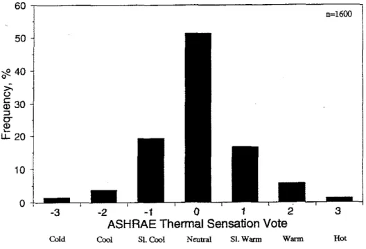
Figure 20 shows the frequency of responses to the ASHRAE thermal sensation question. The response frequencies form a normal distribution (skewness = 0.045, not significantly different from zero, z = 0.735). The modal response was '0' or 'neutral' (n=1600), this response represented 51.3 % of the recorded responses. Figure 21 shows the frequency of votes in the central category ('0') and the central three categories ('-I,, 'O', '+1') of the ASHRAE thermal sensation scale at each indoor air temperature. In this Figure the ASHRAE votes were grouped according to the corresponding indoor air temperature. The mean ASHRAE vote in each 1 OC temperature bin was then calculated. Then the mean vote of each bin was plotted vs. the mean temperature of the bin. The peak for both curves occurs for the temperature bin 23.1 - 24 OC, with a mean bin temperature of 23.4 "C. Figure 22 shows the cumulative frequencies of votes on the ASHRAE thermal sensation scale. Again, the cumulative frequencies were plotted vs. mean bin
temperatures, as in Figure 22. Each curve represents the percentage of votes in any of the categories labeled below the curve.
Figure 23 shows the frequency of responses to the McIntyre thermal preference question (see Appendix A). The response frequencies form a normal distribution (skewness = 0.033,not significantly different from zero, z = 0.539). The modal response was
'0'
or 'no change' (n=1599), this response represented 69.6 % of the recorded responses. Figure 24 shows the frequency of votes in each of the McIntyre thermal preference categories at each indoorair
temperature; the Figure was constructed in the same way as Figure 21. The peak for the 'no change' curve occurs for the temperature bin 23.1 - 24 "C, with a mean bin temperature of 23.4 "C.Figure 25 shows the frequency of responses to the question regarding clothing modification (see Appendix A). The modal response was 0 or 'none' (n=1601), this response represented 85.3 % of the recorded responses.
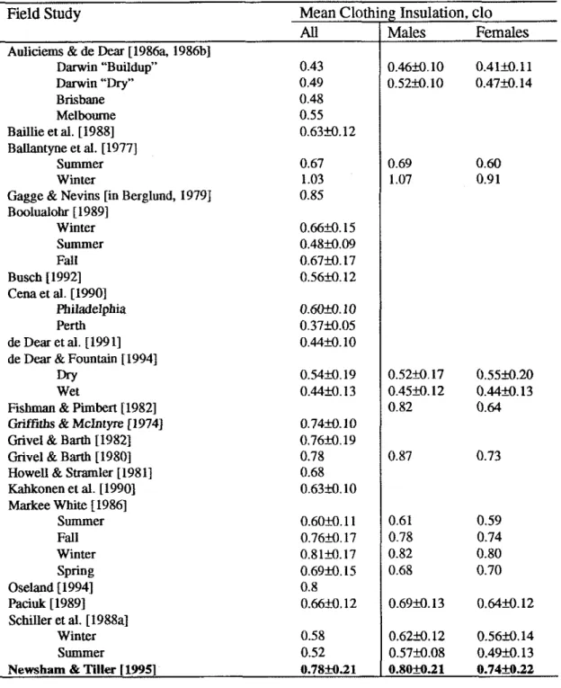
Figure 26 shows the frequency of responses to the question regarding clothing insulation worn at the start of the working day (see Appendix A). For Figure 26, clothing insulation was sorted into 0.1 clo bins. The mean clothing insulation worn was 0.78 (n = 1250), s.d. = 0.21. The frequency distribution is bimodal. The first peak occurs for a clothing insulation of 0.61 to 0.7 clo, the second at 1.01 to 1.1 clo.
A Field Study of Oflice Thermal Cornfin Newsham & Tiller 16
Interpreting the responses to the question regarding clothing worn was more difficult than interpreting the responses to any of the other questions. The question asked 'What
clothing were you wearing when you arrived at work today'. Clearly, the response to this question should not change within a day, yet limitations of ScreenSurvey meant that this question was asked twice per day,
l i e
all the other questions. Some participants answered twice in a day, while others ignored it if it appeared a second time in the same day. To avoid weighting the data towards those who answered the question more than once ina
day, we post-processed the data, removing (for this question only) any data which represented a particular participant's second response to this question on aparticular day. In cases where the participant answered the question more than once in a day and gave a different response each time, we assumed that the response representing the higher level of clothing insulation was the valid response. This explains why the number of responses to this question is substantially lower than the number of responses to the thermal sensation, thermal preference, and clothing change questions.
The question required the participants to complete a checklist of clothing items. To be of use in a quantitative sense, the completed checklist had to be converted into an equivalent clothing insulation. To do this, we used the insulation values from ANSUASHRAE 55-
1992 [ib92], with some slight modifications, as detailed in Table 5. Following ANSIIASHRAE 55-1992, we assumed:
LI
=I:
LI"
where,
LI
= total clothing insulation of ensemble, clo, ,
= clothing insulation of individual item, cloSome participants expressed reluctance to detail information regarding certain items of clothing (see Section 4.12), and did not include them in their responses. On other
occasions it appeared that participants simply mistakenly omitted clothing items from their completed checklist. We thought it reasonable to assume that the following items of clothing were being worn, even if omitted from the occupants response: briefs, either shoes or sandals, either dress or skirt or pants or shorts. If these items were missing, then in post-processing we added clothing insulation values for briefs, shoes, skirt (if female) and pants (if male).
Our clothing checklist was also very generic. Clothing thermal resistance is governed by many factors, including: thickness, porosity, textile fibre, air layers, body posture, vapour diffusion, fit, layering, surface finish, activity of wearer [Boonlualohr, 1989; Goldman, 1980; Markee White, 1986; McCullough et al., 1994; Olesen, 1985; Oseland &
Hurnphreys, 19931. However, we judged that any attempt to capture this information in our study would have made the questionnaire too cumbersome to be administered on a frequent basis.
A Field Study of Office 7'herml Comfon Newsham & Tiller 17
Table 5. Items on the clothing checklist and their clothing insulation values.
Description
I&,
cl0 NotesBraICarnisole 0.01 ANSUASHRAE contains no value for camisole
T-shirt Briefs Long Underwear Half Slip Full Slip Socks Pantyhose Sandals ShoeslBoots Tielscarf
Short Sleeved Shirt Long Sleeved Shirt Dress Skirt Pants Shorts Sweater Vest Jacket
Includes women's underwear
Assuming ankle socks value from ANSUASHRAE
Assuming shoes value from ANSUASHRAE
Guess, no value in ANSUASHRAE, tightens collar fit Assuming knit sports shin value from ANSVASHRAE
Mean of dress shin and flaunel shirt value from ANSUASHRAE Assuming long sleeved thin dress value from ANSVASHRAE Mean of thin s k i i and thick skii value from ANSIIASHRAE Assuming thick pants value from ANSUASHRAE
Assuming walking shorts value from ANSVASHRAE Mean of sweatshin and long-sleeve sweater, ANSIIASHRAE Mean of thin vest and thick vest value from ANSUASHRAE Assuming single-breasted thick jacket from ANSUASHRAE
Clearly, there is a lot of uncertainty in the derived clothing insulation values.
Figure 27 shows the frequency of responses to the question regarding blind position (Appendix A). The mean blind position was 0.54 (n = 11 1 I), s.d. = 0.40. The frequency distribution is bimodal, at responses indicating blinds fully open (1) or fully closed (0). Blinds were fully open 31 % of the time, and fully closed 20 % of the time.
Obviously, this question was only relevant to those participants with windows at their workstations; limitations of ScreenSurvey meant that this question was asked of all
participants. Participants who did not have windows at their workstations were instructed to ignore this question.(see Appendix A). However, some participants without windows did answer if presumably giving a value for a distant window they could see from their workstation. In post-processing the data, we removed (for this question only) any data from participants without windows at their workstations. This explains why the number of responses to this question is substantially lower than the number of responses to the thermal sensation, thermal preference, and clothing change questions.
A Field Study of Once lkermal Comfort Newsham & Tiller 18
3.5 Order Effect
We tested whether the order in which the ASHRAE thermal sensation and McIntvre thermal preference questions were asked influenced the responses. For each participant, we examined ASHRAE votes when the concurrent McIntyre vote was '0' ('no change'). We divided the ASHRAE votes into two 'order groups': those made when the McIntyre question was asked before the ASHRAE question, and those made when the ASHRAE question was asked before the McIntyre question. Then, for each participant, we calculated the mean ASHRAE vote for each order arouD (note, the number of votes in
-
a .each group differed by group and by participant). We then used the Wilcoxon Signed Ranks method to test for differences between the two order groups. Differences in ASHRAE vote by order of question presentation were not significant (z = -0.736, p = 0.46, n = 51).
Note that the total number of occasions when the ASHRAE question was asked fust was less than half of the occasions when the McIntyre question was asked fust. Appendix B shows that the TMES.DAT files scheduled the ASHRAE question ahead of the McIntyre question only 40 % of the time. Further, the times at which the ASHRAE question was asked before the McIntyre question tended to cluster around early morning and late afternoon, when the participant may not have been at work.
3.6 Correlations between Data
Table 6 shows the correlation coefficients (r) between several of the participant-related and physical parameters and votes on the ASHRAE thermal sensation and McIntyre thermal preference questions. Responses from all participants have been grouped. Only occasions where responses to both questions were made are considered.
Table 6. Correlation coefjicients (r) between variables.
*
indicates significant at the 0.05 level,**
indicates significant at the 0.01 level.n = 1544 ASHRAE McIntyre Clo-change Clo
Participant- ASHRAE related McIntyre -0.712 ** Clo-change -0.203
**
0.179 ** Clo 0.025 0.010 -0.130 ** . . .. .. .. ... .. ... . .. . .. . ... ... .......
.. . . ... ... .. . .. ... ... ... .. . .. , .. ...
. .. . .. ....
. .. . .. . .. . ... ... .. . .. . . . , . .. . .. .. . . ... . . .. . . . .. . . . .. . . .. . . .. ... ..
, . ... . . .. . . ... . . .. . .. . . . Physical Ind-ai-temp 0.335 ** -0.303 ** -0.189 ** -0.045 Ind-humid 0.005 -0.032 0.061 * -0.013 Out-air-temp 0.122**
-0.148 ** -0.058 * -0.085**
Out-humid -0.123**
0.103 ** 0.055 * -0.014 Tot-horiz-solar 0.165**
-0.137**
-0.064 * -0.0433.7 Regressions between Participant Responses and Physical Measures
Figure 28 shows a bubble plot of all the individual responses to the ASHRAE thermal sensation question vs. the corresponding indoor air temperature. A bubble plot is a variation on the scatter plot where the size of the bubble is proportional to the number of
A Field Study of Once Thermal Comfort Newsham & Tiller I 9
data points at a particular location on the plot A regression line is drawn through the data, and has the equation:
where,
TS = ASHRAE thermal sensation vote Tia = Indoor
air
temperature (OC)Note that in performing this regression we are defying the strict requirements of linear regression models, which require an equal-interval-type dependent variable [de Dear &
Auliciems, 19851. The ASHRAE thermal sensation scale is ordinal: the responses are unambiguously ordered, but the width of each category is not necessarily the same (see Figure 22). In the case of such ordinal scales Probit analysis is more appropriate [de Dear, 19941. However, grouped data collected using the ASHRAE scale are commonly treated
as
if collected using a continuous, equal-interval scale, and studies that have used both this treatment and probit analysis have found very similar results [McIntyre, 19781.Figure 29 shows a more traditional plot of the same data. In this Figure the ASHRAE votes were grouped according to the corresponding indoor air temperature bin. The mean ASHRAE vote in each bin was calculated. Finally, the mean vote of each bin was plotted vs. the mean temperature of the bin. Also shown on the Figure are the number of data points in each bin, the standard deviations in the ASHRAE votes for each bin (represented by the error bars), and a regression line. The regression l i e is weighted according to the number of observations associated with each mean, and has the equation:
TS = -7.56
+
0.33 Ti. (n = 1600,? = 0 . 7 7 , ~<
0.001) (3) If we calculate the regression line without weighting each point according to the number of observations, the regression equation becomes:TS = -8.04
+
0.36 Ti. (n = 8, r2 = 0.73, p = 0.007) (4) A regression of the McIntyre thermal preference votes vs. indoor air temperature,analogous to Equation 2 has the equation:
where,
TP = McIntyre thermal preference vote
Figure 30 shows (like Figure 29) the mean McIntyre vote in each indoor
air
temperature bin vs. the mean temperature of the bin. Also shown on the Figure are the number of dataA Field Study of Office Thermal Comfofl Newshnm & Tiller 20
points in each bin, the standard deviations in the McIntyre votes for each bin (represented by the enor bars), and a regression line. The regression line is weighted according to the number of observations associated with each mean, and has the equation:
If we calculate the regression line without weighting each point according to the number of observations, the regression equation becomes:
A multiple regression of the individual ASHRAE thermal sensation votes on the following variables: clothing insulation, measured indoor air temperature, indoor relative humidity, outdoor air temperature, outdoor relative humidity, total horizontal solar radiation, calculated vertical solar radiation on the relevant orientation, and forecast temperature (outdoor air temperature at 8 am each morning, a temperature that might have influenced morning clothing choice) did not substantially increase
9
over using indoor airtemperature alone
(2
= 0.14 vs.?
= 0.1 1, see Eq. 2).Figure 31 is a plot of mean weekly ASHRAE vote vs. mean weekly forecast temperature. The regression line through the scatter points has the equation:
where,
T f = Forecast air temperature ("C)
3.8 The Effect of Response Rate on Regressions
In the correlations and regressions of Sections 3.6 and 3.7 we grouped all responses into a single data
set.
However, Figure 16 shows quite clearly that each respondent voted a different number of times. It is reasonable to ask whether it is appropriate to group the data given that the respondents with a greater response rate will be more represented in the data set than the respondents who voted less frequently.We addressed this issue in two, essentially equivalent ways. First, we regressed ASHRAE vote on indoor
air
temperature for each participant. We then plotted, for each participant, the mean square residual, MS~~idval (variance in ASHRAE vote not accounted for by indoor air temperature) vs. the number of responses; this graph is shown in Figure 32. There appears to be no correlation between MS~uid~at and response rate, and this was confmed by an F-test (F = 0.008, n = 54,? < 0.001,p = 0.93). Secondly, we created a new variable "Number of Votes" and performed a multiple regression for the grouped data set, regressing ASHRAE vote on indoor air temperature and Number of Votes. Note, if a particular participant made 20 votes, that participant would contribute 20 potentiallyA Field Study of Ofjie Thermal Comfon Newsham & Tiller 21
different ASHRAE votes and corresponding indoor air temperatures to the data set, but their value for the Number of Votes variable would be the same in each case (= 20). While the t-test for the regression coefficient associated with temperature was highly significant, the t-test for the regression coefficient associated with Number of Votes was not significant (t = -0.064, n = 1600, p = 0.55).
Since response rate appears to have no significant effect on ASHRAE vote, we conclude that it was appropriate to group all the response data for the purposes of the correlations and regressions of Sections 3.6 and 3.7.
3.9 Neutral and Preferred Temperatures
The neutral temperature
en)
is the indoor air temperature most likely to produce the response '0' or 'neutral' on the ASHRAE thermal sensation scale. T. can be derived in two ways. F i t , from the regression of Equations 2 , 3 and 4; second, from the frequency distribution of Figure 21. Inserting the value TS = 0 into Equations 2 , 3 and 4 yields a T. of 22.7 OC, 22.9 OC, and 22.3 OC respectively. Figure 21 shows that the temperature bin with the highest frequency of 'neutral' responses was 23 - 24 OC.The preferred temperature CT,) is the indoor air temperature most likely to produce the response '0' or 'no change' on the McIntyre thermal preference scale. Tp can be derived in the same two ways as T.. Inserting the value TP = 0 into Equations 5 , 6 and 7 yields a T, of 22.7 "C, 23.1 OC, and 23.0 OC respectively. Figure 24 shows that the temperature bin with the highest frequency of 'no change' responses was 23
-
24 OC.3.10 Comparison with Predicted
Mean
Vote (PMV)PMV is the mean thermal sensation vote for a population as predicted from Fanger's thermal comfort equations Fgnger, 19701. We calculated the PMV associated with each questionnaire response using Sherman's simplification of Fanger's equations [Sherman,
19851. As inputs to the equations, we used the measured values of indoor temperature, humidity, and reported clothing (with the addition of 0.15 clo to account for the insulative value of an office chair,
as
recommended in Brager et al. [1994]; de Dear & Fountain [1994]; McCullough et al. 119941; Palonen et al. [1993]), and assumed mean radiant temperature equal to air temperature, an air velocity2 of 0.1 ms-I, and an activity3 of 1.2This is a common assumption for the oftice environment. Several studies have measured air velocity in the field, and reported the following values (in ms-I):
Auliciems & de Dear [1986b], Darwin "Buildup": 0.14, Darwin "Dry": 0.07; Baillie et al. 119881:
-
0.1; Boyce [1974]: 0.12; Busch [1990]: 0.12; Croome et al. 119921: 0.08; de Dear & Auliciems [1985], Brisbane: 0.15, Melbourne: 0.11; de Dear et al. [1991]: 0.11; de Dear & Fountain 119941, "Dry": 0.12N- .03, "Wet": 0.13M.04; Grivel & Bartb [1980]: 0.07; Kahkonen et al. [1990]: 0.083.03; Markee White 119861: 0.11M.05; Oseland [1994]: 0.10; Palonen et al. (19931: <0.05; Schiller et al. [1988a], Winter: 0.063.05, Summer 0.10+0.09.This is the mean value commonly assumed for office work. Several field studies have tried to measure mean metabolic rate in the office through participant self report of recent activity, and reported the following values in met units (1 met = 58.2 ~ m - ' ) :
A Field Study of Ofice Thermal Comfort Newsham & Tiller 22
met. These assumptions clearly introduce uncertainty into the calculation of PMV. Figure 33 compares our reported mean ASHRAE vote and mean PMV in each
temperature bin. Also shown on Figure 33 are regression lines through the two sets of points. The regression equation for the PMV data, without weighting for the number of observations in each temperature bin, is:
PMV = -4.73
+
0.22 Ti. (n = 8, rZ = 0 . 9 9 , ~ < 0.001) (10) 3.11 Differences between Demographic GroupingsIn this section the data are presented after being sub-divided into appropriate site-based and demographic-based groups.
Table 7 shows the mean indoor air temperature at each of the four sites; this is for the subset of indoor air temperatures measured at the time that the ASHRAE thermal
sensation question was answered by at least one participant at the site. Table 7 shows, for each site, the number of responses, the mean indoor air temperature, and the standard deviation in the mean indoor air temperature. It also shows the results of an analysis of variance between sites.
Table 7. Mean indoor air temperature measured at each site. A lower-case letter in the ANOVA row indicates the site is significantly different at the 5 % level from the sire with
the same letter in upper case, as determined by an analysis of variance.
Site 1 2 3 4
n
337 374 847 42 mean, "C 23.0 23.3 22.4 23.3 s.d., O C 0.9 0.4 1.1 0.4 ANOVA A a B a b C cThere was a difference between the mean indoor air temDerature of UD to 1.0 OC between
sites. Note, the highest standard deviation was observed at Site 3, where temperatures were recorded at five different locations; the lowest standard deviation was observed at Site 4, where temperatures were recorded at only one location, and the number of observations was relatively small.
Table 8 shows the mean indoor air temperature for each orientation at Site 3. Table 8 shows, for each orientation, the number of responses, the mean indoor air temperature, and the standard deviation in the mean indoor air temperature. It also shows the results of
Baillieet al. [1988]: 1.4M.3; Brager etal. [1994]: 1.1; Cenaet al. [1990], Philadelphia: 1.6H.5, Perth: 1.6M.2; de Dear et al. [1991]: 1.2; de Dear & Fountain [1994]: 1 . 3 3 . 2 ; Grivel & Barth 119821: 1 . 7 3 . 3 ; Grivel & Barth [1980]: 1.2; Markee White [1986]: 1 . 1 3 . 1 ; Oseland [1994]: 1.2.
A Field Study of Ofice T h e m 1 Comfon Newshorn & Tiller 23
an analysis of variance between orientations.
Table 8. Mean indoor air temperature measured for each orientation at each Site 3. A lower-case letter in the ANOVA row indicates the orientation is significantly different at the 5 % levelfrom the orientation with the same letter in upper case, as determined by an
analysis of variance. Site 3
east north south west
n 150 113 20 1 112
mean. OC 22.6 21.8 22.4 22.3
Table 9 shows the mean response to the ASHRAE thermal sensation question at each site. Table 9 shows, for each site, the number of responses, the mean ASHRAE vote, and the standard deviation in the mean ASHRAE vote. It also shows the results of an analysis of variance between sites. Site 4 is not shown because there was only one participant at this site making comparisons to other sites meaningless.
Table 9. Mean ASHRAE vote recorded at each site. A lower-case letter in the ANOVA row indicates the site is significantly different at the 5 % levelfrom the site with the same
letter in upper case, as determined by an analysis of variance. Site
mean vote 0.28 -0.12 -0.03
s.d. 0.97 0.79 1.09
ANOVA A a a
Figure 34 shows the frequency of responses to the ASHRAE thermal sensation question at each site; Site 4 was excluded because of the relatively small number of responses (n = 42). The modal response was 0 or 'neutral' at each of the sites. The data from Site 1 are skewed significantly toward warm responses (skewness = 0.577,
n
= 337, z = 4.32). AxZ
test shows that the distribution of ASHRAE votes differed significantly between all site pairs,as
detailed in Table 10.Table 10.
x2
test of ASHRAE vote distributions painvise by site. Sitex2
value 38.5 39.0 44.8A Field Study of Omce Thermal Cornfin Newshum & Tiller 24
Table 11 shows the mean response to the ASHRAE thermal sensation question for each sex. Table 11 shows, for each sex, the number of responses, the mean ASHRAE vote, and the standard deviation in the mean ASHRAE vote. It also shows the results of an analysis of variance between sites.
Table I I . Mean
ASHRAE
vote by sex.A
lower-case letter in the ANOVA row indicates the sex is significantly different at the 5 % level from the sex with the same letter in uppercase, as determined by an analysis of variance.
Sex female male n 712 80 1 mean vote -0.12 0.08 s.d. 1.02 0.94 ANOVA A a
Figure 35 shows the frequency of responses to the ASHRAE thermal sensation question of each sex. The modal response was 0 or 'neutral' at each of the sites. A
xZ
test shows the two dislributions to be significantly different(xZ
= 23.9, df = 6, p = 0.001)Table 12 shows, for each age category, the number of responses, the mean ASHRAE vote, and the standard deviation in the mean ASHRAE vote. An analysis of variance indicated no significant difference in mean vote between age categories (category 60
-
69 was excluded from the analysis of variance because the data came from a single participant only).Table 12. Mean
ASHRAE
vote by age.mean vote -0.01 0.03 -0.07 -0.04 0.69
s.d. 1.04 1.07 0.93 0.55 0.95
Table 13 shows the mean response to the ASHRAE thermal sensation question for each orientation. Only responses from Site 3
are
shown, as this was the only site withparticipants with offices in
d
four orientations. Further, only responses from participants whose offices had an outside window were included. Table 13 shows, for eachorientation, the number of responses, the mean ASHRAE vote, and the standard deviation in the mean vote. An analysis of variance indicated no significant difference in mean vote between sites.
Table 13. Mean ASHRAE vote by orientation at Site 3.
Site
East North South West
n 150 113 20 1 112
mean vote 0.02 -0.04 0.15 0.05
s.d. 0.97 0.93 1.12 0.90
Table 14 shows the mean clothing insulation worn to work, by site. Site 4 is not shown because there was only one participant at this site making comparisons to other sites meaningless in this case. Table 14 shows, for each site, the number of responses, the mean clothing insulation, and the standard deviation in the mean clothing insulation. An analysis of variance showed no significant difference between the clothing insulation adopted at each of the sites, at the 5 % level.
Table 14. Mean clothing insulation reported at each site.
Site
m "
n 267 295 65 1
mean clo 0.79 0.76 0.79
s.d. 0.21 0.25 0.20
Table 15 shows the mean clothing insulation worn to work, for each sex (remember that only 50 of the 55 participants identified themselves by sex). Table 15 shows, for each sex, the number of observations, the mean clothing insulation, and the standard deviation in the mean clothing insulation. It also shows the results of an analysis of variance between sites.
Table 15. Mean reported clothing insulation by sex. A lower-case letter in the ANOVA row indicates the sex is significantly different at the 5 % level from the sex with the same
letter in upper case, as determined by an analysis of variance.
Sex female male n 553 622 mean clo 0.74 0.80 s.d. 0.22 0.21 ANOVA A a
Figure 36 shows the mean reported blind position for each site and for each orientation; only those responses from participants whose offices had external windows were included. Both Site 2 and Site 3 had south facing offices; at Site 2 the mean blind position was 0.30 (n = 209), s.d. = 0.33, whereas at Site 3 the mean blind position was 0.52 (n = 200). s.d. = 0.40; an analysis of variance indicated that the two were significantly different (F = 3 9 . 9 , ~
<
0.001). Site 1 and Site 3 had west facing offices; at Site 1 the mean blind position wasA Field Sfudy of Ofice Thermal Comforf Newsham & Tiller 26
0.10 (n = 155). s.d. = 0.18, whereas at Site 3 the mean blind position was 0.65 (n = 113), s.d. = 0.32; an analysis of variance indicated that the two were significantly different (F = 3 1 8 . 6 , ~
<
0.001).The data from Site 3 only reveals that there was also a difference in mean blind position between orientations. The mean blind positions for the south and west facing offices are lower than those for the east (mean = 0.80, n = 150, s.d. = 0.31) and north (mean = 0.95, n = 114, s.d. = 0.13) facing offices. A pairwise analysis of variance indicated significant differences in blind position between all orientations @ < 0.01)
3.12 Longitudinal Data
Figure 37 shows the weekly (Monday to Friday.) mean response to the ASHRAE thermal sensation question for all four sites. The standard deviation in the weekly data is indicated by the error bars. There may be a slight tendency for mean response to decrease with time (as the outdoor climate gets colder), though the week ending November 4th is an obvious exception to this. We tested this tendency by collapsing the ASHRAE votes into two sub- sets: those of the first five weeks of the study (mean = 0.09, n = 854). and those from the second half (mean = -0.09, n = 746). The two sub-sets were then compared by an analysis of variance, which showed them to be significantly different (n = 1600, F = 13.0, p < 0.001).
Figure 38 shows the hourly mean response to the ASHRAE thermal sensation question for all four sites and for all 10 weeks of the study period. The standard deviation in the hourly data is indicated by the error bars. There may be a slight tendency for mean response to increase in the afternoon. We tested this tendency by collapsing the ASHRAE votes into two sub-sets: those of hours 9 to 12 (morning, mean = -0.09, n = 7 15). and those of hours 13 to 16 (afternoon, mean = 0.13, n = 780); hours 17 and 18 were excluded because of their small data sets, n17+,s = 105. The two sub-sets were then compared by an analysis of variance, which showed them to be significantly different (n = 1495, F = 18.5, p < 0.001). Figure 39 shows the mean response to the ASHRAE thermal sensation question in the morning and afternoon for each orientation at Site 3 (the only site with participants in offices with windows facing the 4 cardinal directions) and for all 10 weeks of the study period. An analysis of variance showed that the differences in the means in the morning and afternoon were not significant, except for the south orientation (n = 185, F = 8.1, p = 0.005). Figures 40 and 41 show a similar plot for the single orientation at Site 1 (west) and Site 2 (south). An analysis of variance showed that the differences in the means in the morning and afternoon were not significant at Site 2, but were significant at Site 1 (n = 154, F = 1 1 . 4 , ~ = 0.001).
Figure 42 shows the weekly mean clothing insulation level value for each sex. Clothing insulation worn by males was consistently slightly higher than clothing insulation worn by females. The mean clothing level for males in the first five weeks of the study was 0.79 clo (n = 3321, slightly lower than that in the second five weeks, 0.82 clo (n = 290). The
A Field Study of Office Thermal Comfort Newsham & Tiller 27
mean clothing level for females in the first five weeks of the study was 0.72 clo (n = 283), slightly lower than that in the second five weeks, 0.76 clo (n = 270). However, an analysis of variance indicated that these differences were not significant at the 5 % level.
3.13 Analysis of Final Evaluation Questionnaire
Figures 43 to 48 show the frequency distribution of responses to the final evaluation questionnaire.
As described in Section 2.6, a Warning Banner window appeared on screen prior to the thermal comfort question. The Warning Banner informed the participant that the
questionnaire was due to be administered and gave them the opportunity to postpone the questionnaire. When asked if they found the appearance of the Warning Banner obtrusive, Figure 43 shows that only 4 % of respondents voted 3 or 4 on the 5 point scale (0 = 'not at all', 4 = 'very'). Further, when asked about the size of the Warning Banner (the question screens were the same size as the Warning Banner), Figure 44 shows that 90 %
of respondents found the size of the Warning Banner 'acceptable'. Figure 45 shows the responses to perhaps the most pertinent of the follow-up questions, 'Did this method of automatic questionnaire administration distract you from your work?' Figure 45 shows that only 11 9% of respondents voted 3 or 4 on the 5 point scale (0 = 'not at all', 4 = 'very much'). When asked about the number of questions asked at each scheduled time, Figure 46 shows that 79 % of respondents found the number of questions 'acceptable', whereas
19 % thought 'too many' questions were asked each time. When asked if the
questionnaire appeared too often, Figure 47 shows that only 6 % of respondents said 'Yes'. Finally, when asked if they would have liked to make the questionnaire appear on demand (remember, in our study the questionnaire appeared according to an experimenter defined schedule), Figure 48 shows that 75 % said 'No', and '25 % said 'Yes'.
A Field Study of Offce Thermal Comfoa Newsham & Tiller 28
4.0 Discussion
This section contains discussion of the results presented in Section 3. 4.1 Frequency of Response
The principal aim of this study was to evaluate the software as a technique for delivering suestionnaires. Figure 16 shows that the mean reswnse rate was 29.1 A
-
%. This means that each participant answered the questions an average of 29 times during the ten week period, not that only 29 % of participants responded (in fact all 55 participants responded at least twice over the study period). Thus, the volume of data collected was actually relatively high, over 1500 data points for several of the questions, and was in-line with our expectations. By comparison, Humphreys and Mcol [I9701 used voting hardware to poll participants hourly for 15 months and obtained an overall response rate of about 11 %.There was no evidence to indicate that the software malfunctioned during the study period. Therefore, the only possible reasons why the response rate was not higher are:
1. The participants were at work but their computers were not switched on. 2. The participants were at work but did not respond to the questionnaire when it
appeared; they were away from their desks temporarily, or canceled the questionnaire when it appeared.
3. Participants were not at work and their computers were not switched on. It is unlikely that the first reason contributes to a reduction in response rate. Other research [Newsham & Tiler, 19941 shows that workers at these and other similar sites have their computers switched on all of the time they
are
at work.The data file recorded when there was no response to the questionnaire when it appeared. Over the survey period this occurred on 22.8 % of the occasions when the questionnaire was presented. Only on a few occasions did the participant actively cancel the
questionnaire, therefore we can assume that the lack of response was due to occupants being temporarily absent from their desks (the questionnaire "timed out" if there was no response within 1 minute of appearing). Thus, we can infer from these data that our sample of participants were temporarily away from their desks about 20 % of a typical working week.
Since we know the response rate to the questionnaire (29.1 %), and the "no response" rate (22.8 %), the remainder (48.1 %) are occasions when the questionnaire was
scheduled to appear but for which no data were recorded in the data file. This could only happen if the computer was not switched on at the scheduled time, which almost certainly means the participant was not in the building (on travel, working at another site, on leave etc.). Questionnaires were scheduled to appear at regular intervals from 0800 hrs to 1800
A Field Study of Ofice Thermal Comfort Newsham & Tiller 29
hrs, which covers 10 hours, whereas a typical working day might only cover 8 hours. Therefore we might expect a missing data rate of 20 % due to question scheduling alone. Vacation leave might normally account for another 5 %. That still leaves a large degree of absenteeism. We have no evidence to suggest that this absenteeism is anything other than legitimate. Neither do we know whether the high degree of absenteeism is due to the nature of our participants' jobs, or if it is representative of modem office workers in general. Opdal & Brekke [1995], observing nine Norwegian offices, found workers away from their desks 72 % of the working week! While these findings are of no direct
consequence to thermal comfort, it may be useful data to those constructing occupancy profies for office buildings.
4.2 Comparison of Frequency Data with Thermal Comfort Standards
ANSUASHRAE [I9921 and I S 0 Standards [I9841 have requirements for acceptable indoor thermal comfort conditions. The goal of these standards is that 80 % of the occupants should be satisfied. Satisfaction is defined as being a vote in the central three categories (-1,0, +1, or 'slightly cool', 'neutral', 'slightly warm') of the ASHRAE thermal sensation scale. The standards use Fanger's
P M V
model [I9701 to derive acceptable operative temperature ranges based on the above goal, given assumptions for the other environmental and personal variables required by Fanger's model. Table 16 shows the required temperature ranges, and assumptions, by season. Note, Table 16 quotes the required temperature ranges for 10 % dissatisfaction whereas the overall goal of the standard is to achieve the less stringent 20 % dissatisfaction. Presumably the temperature requirements in the standards are more rigorous to allow for some variation of conditions spatially within the building, and for values for other physical and personal parameters that differ from the assumptions within the population.Table 16. ANSI/ASHRAE and IS0 Standard acceptable operative temperatures for thermal comfort, by seuson [ANSI/ASHRAE, 1992; ISO, 19841.
Season Optimum Range for 10 % Assumptions
~imperature, O C ~issksfaction, "C
winter 22.0 20.0 to 23.5 RH=50 %, mean air speed S 0.15 m..',
1.2 met. 0.9 clo
Summer 24.5 23.0 to 26.0 RH=50 %, mean air speed
<
0.15 m-',Figure 20 shows that in our study, 87 % of responses to the ASHRAE thermal sensation question were within the central three categories. This indicates that, according to ASHRAE and I S 0 standards, the sites as a whole exhibited acceptable thermal comfort. But was this acceptable thermal comfort achieved by adhering to the temperature ranges specified in the Standards? Although our study was conducted during winter, the mean clothing insulation we recorded was 0.78 clo, less than the 0.9 clo assumption of the