HAL Id: hal-00317681
https://hal.archives-ouvertes.fr/hal-00317681
Submitted on 3 Nov 2004
HAL is a multi-disciplinary open access
archive for the deposit and dissemination of
sci-entific research documents, whether they are
pub-lished or not. The documents may come from
teaching and research institutions in France or
abroad, or from public or private research centers.
L’archive ouverte pluridisciplinaire HAL, est
destinée au dépôt et à la diffusion de documents
scientifiques de niveau recherche, publiés ou non,
émanant des établissements d’enseignement et de
recherche français ou étrangers, des laboratoires
publics ou privés.
ionosphere during the geomagnetic storm of 25-27
August 1987
A. V. Pavlov, S. Fukao, S. Kawamura
To cite this version:
A. V. Pavlov, S. Fukao, S. Kawamura. F-region ionospheric perturbations in the low-latitude
iono-sphere during the geomagnetic storm of 25-27 August 1987. Annales Geophysicae, European
Geo-sciences Union, 2004, 22 (10), pp.3479-3501. �hal-00317681�
SRef-ID: 1432-0576/ag/2004-22-3479 © European Geosciences Union 2004
Annales
Geophysicae
F
-region ionospheric perturbations in the low-latitude ionosphere
during the geomagnetic storm of 25–27 August 1987
A. V. Pavlov1, S. Fukao2, and S. Kawamura3
1Inst. of Terrestrial Magnetism, Ionosphere and Radio-Wave Propag., Russian Academy of Science, Troitsk, 142 190, Russia 2Research Institute for Sustainable Humanosphere, Kyoto University, Uji, Kyoto 611-0011, Japan
3National Institute of Information and Communications Technology, 4-2-1, Nukui-kita, Koganei, Tokyo 184-8795, Japan
Received: 10 February 2004 – Revised: 8 June 2004 – Accepted: 2 July 2004 – Published: 3 November 2004
Abstract. We have presented a comparison between the
modeled N mF 2 and hmF 2, and N mF 2 and hmF 2 which were observed at the equatorial anomaly crest and close to the geomagnetic equator simultaneously by the Akita, Kokubunji, Yamagawa, Okinawa, Manila, Vanimo, and Dar-win ionospheric sounders and by the middle and upper at-mosphere (MU) radar (34.85◦N, 136.10◦E) during the 25– 27 August 1987 geomagnetically storm-time period at low solar activity near 201◦, geomagnetic longitude. A compari-son between the electron and ion temperatures measured by the MU radar and those produced by the model of the iono-sphere and plasmaiono-sphere is presented. The corrections of the storm-time zonal electric field, E3, from 16:30 UT to 21:00 UT on 25 August bring the modeled and measured hmF2 into reasonable agreement. In both hemispheres, the meridional neutral wind, W, taken from the HWW90 wind model and the NRLMSISE-00 neutral temperature, Tn, and densities are corrected so that the model results agree with the ionospheric sounders and MU radar observations. The geomagnetic latitude variations in N mF 2 on 26 August dif-fer significantly from those on 25 and 27 August. The equa-torial plasma fountain undergoes significant inhibition on 26 August. This suppression of the equatorial anomaly on 26 August is not due to a reduction in the meridional compo-nent of the plasma drift perpendicular to the geomagnetic field direction, but is due to the action of storm-time changes in neutral winds and densities on the plasma fountain pro-cess. The asymmetry in W determines most of the north-south asymmetry in hmF 2 and N mF 2 on 25 and 27 August between about 01:00–01:30 UT and about 14:00 UT when the equatorial anomaly exists in the ionosphere, while asym-metries in W, Tn, and neutral densities relative to the geo-magnetic equator are responsible for the north-south asym-metry in N mF 2 and hmF 2 on 26 August. A theory of the primary mechanisms causing the morning and evening peaks in the electron temperature, Te, is developed. An
appear-Correspondence to: A. V. Pavlov (pavlov@izmiran.rssi.ru)
ance, magnitude variations, latitude variations, and a disap-pearance of the morning Te peaks during 25–27 August are caused by variations in E3, thermospheric composition, Tn, and W. The magnitude of the evening Te peak and its time location are decreased with the lowering of the geomagnetic latitude due to the weakening of the effect of the plasma drift caused by W on the electron density. The difference between 25 August and 26–27 August in an appearance, magnitude and latitude variations, and a disappearance of the evening Tepeak is caused by variations in W, the thermospheric com-position, Tn, and E3.
Key words. Ionosphere (Equatorial ionosphere; electric
fields and currents; plasma temperature and density; iono-spheric disturbances)
1 Introduction
The ionosphere at the geomagnetic equator and low geo-magnetic latitudes is the site of important ionospheric phe-nomena, which include the equatorial electrojet, equatorial plasma fountain, equatorial (Appleton) anomaly, additional layers, plasma bubbles, and spread F . These low-latitude characteristic properties of the ionosphere have been stud-ied observationally and theoretically for many years (Mof-fett, 1979; Anderson, 1981; Walker, 1981; Abdu et al., 1991; Bailey and Balan, 1996; Buonsanto, 1999; Rishbeth, 1975, 2000; Rishbeth and Fukao, 1995; Abdu, 1997, 2001).
A variety of global processes in the iono-sphere/thermosphere/magnetosphere system is generated during geomagnetic storms, and magnetic storm effects on the neutral atmosphere and ionosphere depend on season, latitude, and longitude, as well as on the severity, time of oc-currence, and duration of the storm (Buonsanto, 1999). The electron number density, Ne, can be decreased or increased in association with a magnetic storm in comparison with a quiet time Ne. In general, the equatorial anomaly is less developed during geomagnetic storm-time periods in
com-parison with the quiet time periods, however, enhancements of the equatorial anomaly have also been reported (Rishbeth, 1975). The geomagnetic storm changes in electric fields, thermospheric winds and neutral composition have been suggested as physical mechanisms to explain the variations in the low-latitude ionosphere, and plasmasphere structure and dynamics (Moffett, 1979; Anderson, 1981; Abdu et al., 1991; Buonsanto, 1999; Rishbeth, 1975, 2000; Rishbeth and Fukao, 1995; Abdu, 1997, 2001).
Geomagnetic storm processes, such as particle precipi-tation and Joule dissipation, lead to thermospheric heating and, as a result, to gravity waves/TIDs, disturbed thermo-spheric winds, and composition changes which reach low-latitude regions with a delay of a few hours from the geo-magnetic storm onset. These perturbation neutral winds pro-duce a part of storm-time changes in the equatorial electric fields through the ionospheric disturbance dynamo (Blanc and Richmond, 1980), while the other part of the storm-time equatorial electric field changes is produced by the so-lar wind-magnetosphere dynamo (Senior and Blanc, 1984; Spiro et al., 1988). The duration of electric field distur-bances varies from tens of minutes to hours (Abdu et al., 1991). In general, the low-latitude electric fields undergo large departures from their quiet time averages during ge-omagnetic storms (Fejer and Scherliess, 1997; Fejer, 2002 and references therein). There are clear indications that a dawn-to-dusk disturbed electric field (i.e. eastward/westward on the day/night sides), penetrated in the equatorial iono-sphere, is associated with a southward turning of the inter-planetary magnetic field component, Bz (Abdu et al., 1991; Abdu, 1997). The intensity and duration of the disturbance electric field is controlled by many factors, such as the time constants of the decay/formation of the shielding charges in the inner magnetosphere, and auroral conductivity (Vasyliu-nas, 1975; Kelley et al., 1979; Gonzales et al., 1983), and, as a result, there are still questions concerning the prediction of the storm-time dependence of ionospheric electric fields (Fejer, 2002).
The storm-time F -region changes in the low-latitude iono-sphere have been identified from F -layer height and fre-quency responses observed by ionosondes (see Abdu, 1997 and references therein). The incoherent scatter radar tech-nique has expanded the range of information obtainable from the low-latitude sounders during geomagnetic storms. The dynamics of the low-latitude ionosphere was observed by the MU radar during the great geomagnetic storms of 6–8 Febru-ary 1986, 20–21 JanuFebru-ary 1989, and 20–23 October 1989 (Oliver et al., 1988, 1991; Reddy et al., 1990). The changes of F -layer electron density observed by the MU radar in the 6–8 February 1986 storm were explained by changes in an influx of ionization from the plasmasphere, modulated by the passage of a large-scale southward traveling gravity wave (Oliver et al., 1988). In the 20–21 January 1989 storm, the observed large changes in the F 2 region peak altitude from 23:00 LT to 02:40 LT were attributed to a large eastward electric field originating at auroral latitudes (Reddy et al., 1990). During the 20–23 October 1989 storm-time period,
the first significant auroral display over Japan since 1960 was observed, and drastically different electron densities were discovered using the four radar beams, separated by about 250 km horizontally in the F -region (Oliver et al., 1991). The Arecibo radar observations of the ionospheric F -region dur-ing the 1–5 May 1995 geomagnetic storm period have shown the possible existance of a poleward expansion of the equa-torial anomaly zone with the northern anomaly crest location close to 29◦ dip latitude (Buonsanto, 1999). Another anoma-lous low-latitude ionospheric feature was observed during 17–18 February 1999 highly disturbed geomagnetic period, when the Arecibo radar has recorded an anomalous night-time ionospheric enhancement in which the nightnight-time value of the F 2 peak electron density exceeded 106cm−3and the F2 peak altitude went above 400 km (Aponte et al., 2000).
The difficulties in theoretical studies of the response of the low-latitude ionosphere and plasmasphere to geomag-netic storms arise due to many competing processes imbed-ded in the production, loss and transport electrons and ions. The earlier simplified theoretical computations (Burge et al., 1973; Chandra and Spencer, 1976) have speculated on the importance of the disturbed neutral winds to the low-latitude ionospheric response to geomagnetic storms, but lack of data and/or model winds has hampered progress. Fesen et al. (1989) studied ionospheric effects in the low-latitude ionosphere during the 22 March 1979 geomagnetic storm period using the model without H+ ions, ignoring electric field perturbations due to the storm, and suggest-ing that the temperatures of electron and ions are equal to the neutral temperature. It follows from the results of Fesen et al. (1989) that the equatorial anomaly may be disrupted by the magnetic storm, and the major factor influencing the storm-time ionospheric behavior is the neutral wind. This point of view was reiterated in recent studies, for example, by Sastri et al. (2000), with particular reference to the well– known storm in early November 1993. The coupled thermo-sphere ionothermo-sphere plasmathermo-sphere electrodynamic model was used by Fuller-Rowell et al. (2002) to model the low-latitude ionosphere and plasmasphere for a hypothetical geomagnetic storm at equinox and high solar activity without taking into account geomagnetic storm disturbances in an electric field. Their model results showed response features of the ther-mosphere and ionosphere as a unique system. In particu-lar, Fuller-Rowell et al. (2002) found an equatorial response within 2 h of the storm onset and made clear the difference between the effects of meridional and zonal winds on the dis-turbed ionosphere.
As far as we know, there are no published comparisons between measurements and theoretical calculations of the low-latitude F -region electron density and temperature dur-ing geomagnetic storms, which would take into account the storm-time changes in the thermospheric wind, the electric field, the neutral composition, and the neutral temperature. In this paper, we present the first study of the complex prob-lem of the low-latitude ionospheric response to the disturbed thermospheric wind, electric field, neutral composition, and neutral temperature.
It follows from the above-mentioned studies that horizon-tal neutral winds cause significant variations in the structure and dynamics of the low-latitude ionosphere and plasmas-phere during geomagnetic storms. In the present work, we continue to investigate the role of horizontal neutral winds in the ionization distribution, plasma dynamics, structuring, and thermal balance of the low-latitude ionosphere in the present case study, in which N mF 2 and hmF 2 are observed simul-taneously close to the same geomagnetic meridian at the geo-magnetic longitudes of 201◦±11◦ by the Akita, Kokubunji, Yamagawa, Okinawa, Manila, Vanimo, and Darwin iono-spheric sounders and by the middle and upper atmosphere (MU) radar at Shigaraki (34.85◦N, 136.10◦E, Japan) during the 25–27 August 1987 geomagnetically storm-time period at solar minimum.
The low-latitude ionosphere undergoes changes as a re-sult of storm-time variations in plasma motion perpendic-ular to the geomagnetic field, B, direction due to an tric field, E, which is generated in the E-region. This elec-tric field affects F -region plasma, causing both ions and electrons to drift in the same direction with a drift veloc-ity, VE=E×B/B2. The zonal component of VE (geomag-netic east-geomag(geomag-netic west component) is thought to have only a negligible effect on the low-latitude plasma densities (Anderson, 1981), and changes in the meridional component (component in the plane of a geomagnetic meridian) of the E×B drift velocity, caused by changes in the zonal elec-tric field, affect the distribution of plasma in the low-latitude ionospheric F -region. During geomagnetic storms, the ver-tical equatorial drift shows significant variability in the mag-nitude (Fejer, 2002), and, as a result, the vertical drift given by the empirical model of Fejer and Scherliess (1997) for the geomagnetically storm-time periods is the averaged ver-tical drift and can differ from the verver-tical drift for the stud-ied geomagnetically disturbed time period. The examination of the model of the meridional component of the drift ve-locity has been driven by the relationship between the zonal electric field and the dynamics of the F 2-layer close to the geomagnetic equator. The present work studies the relation-ship between the zonal electric field and the dynamics of the low-latitude F 2-layer in the low-latitude ionosphere, when N mF2 and hmF 2 are observed simultaneously close to the same geomagnetic meridian by the Akita, Kokubunji, Yam-agawa, Okinawa, Manila, Vanimo, and Darwin ionospheric sounders and by the MU radar during the 25–27 August 1987 geomagnetically storm-time period.
Many theoretical models of the plasmasphere and low-latitude ionosphere were constructed and have been applied to study a wide variety of equatorial ionosphere character-istic properties during geomagnetically quiet conditions (see Moffett, 1979; Anderson, 1981; Walker, 1981; Bailey and Balan, 1996; Rishbeth, 2000; Abdu, 1997, 2001, and refer-ences therein). In the present work, we investigate the torial anomaly geomagnetic storm characteristics (the equa-torial trough, and crest latitudes and magnitudes) from the comparison between the measured and modeled Neand elec-tron temperatures, Te, during 25–27 August 1987 using the
new two-dimensional time dependent model of the low- and middle-latitude plasmasphere and ionosphere (Pavlov, 2003), which employs the updated rate coefficients of chemical re-actions of ions and the updated N2, O2, and O
photoioniza-tion and photoabsorpphotoioniza-tion cross secphotoioniza-tions. Ionospheric models are particularly valuable for investigating the changes that would result, in observed quantities, from changes in individ-ual input parameters, and, therefore, the theoretical study of the ionospheric storm response features is a highly complex task in the absence of the measurements of the disturbed ther-mospheric wind, electric field, neutral composition, and neu-tral temperature for the studied time period at low-latitudes close to 201◦ geomagnetic longitude. Nevertheless, it is pos-sible to evaluate whether or not the storm-time variations of the main ionospheric parameters measured by the iono-spheric sounders and the MU radar are consistent with what is calculated from the model of the ionosphere and plasma-sphere. The model of the ionosphere and plasmasphere of Pavlov (2003) uses the NRLMSISE-00 neutral temperature and density model (Picone et al., 2002) and the HWW90 neu-tral wind model (Hedin et al., 1991) as the model input pa-rameters. As a result, model/data discrepancies can arise due to the possible inability of the neutral atmosphere and wind models to accurately predict the storm-time thermospheric response to the studied time period in the upper atmosphere. We investigate how well the MU radar data and the Akita, Kokubunji, Yamagawa, Okinawa, Manila, Vanimo, and Dar-win ionospheric sounder measurements of electron densities taken during 25–27 August 1987 agree with those calculated by the model of the ionosphere and plasmasphere.
The horizontal neutral wind drives the lowlatitude F -layer plasma along magnetic field lines and causes significant north–south asymmetry in the equatorial ionization anomaly during geomagnetically quiet conditions (Balan and Bailey, 1995; Balan et al., 1997 a,b). As far as the authors know, our investigation is the first theoretical study of the role of variations in the neutral winds, temperature, and densities in producing the north−south asymmetry in the storm-time electron density.
Otsuka et al. (1998) found that the occurrence and strength of the morning and evening peaks in Te over the MU radar depend on altitude, season, and solar activity under magneti-cally quiet conditions during 1986–1995. Pavlov et al. (2004) studied, for the first time, the latitude dependence of the occurrence and strength of the morning and evening peaks in Te and the mechanisms causing these peaks in the low-latitude ionosphere during geomagnetically quiet-time con-ditions of 19–21 March 1988. In this work, we report the first results obtained from a study of the latitude dependence of the occurrence and strength of the morning and evening peaks in Te and the mechanisms causing these peaks in the low-latitude ionosphere during the 25–27 August 1987 geo-magnetically storm-time period. The reliability of the con-clusions is based on the comparison between the measured MU radar and modeled Te, and the use of the updated elec-tron cooling rates (Pavlov, 1998a, b; Pavlov and Berrington, 1999) in the model.
2 Theoretical model
The model of the low- and middle latitude ionosphere and plasmasphere, which is described in detail by Pavlov (2003), calculates number densities, Ni, of O+(4S), H+, NO+, O+2, N+2, O+(2D), O+(2P), O+(4P), and O+(2P*) ions, Ne, Te, and Ti. As the model inputs, the horizontal components of the neutral wind are specified using the HWW90 wind model (Hedin et al., 1991), the model solar EUV fluxes are taken from the EUVAC model (Richards et al., 1994), while neutral densities and temperature are taken from the NRLMSISE-00 model (Picone et al., 2002).
The model calculations are carried out in dipole orthogo-nal curvilinear coordinates q, U, and 3, where q is aligned with, and U and 3 are perpendicular to B, and the U and 3 coordinates are constant along a dipole magnetic field line. It should be noted that q=(RE/R)2cos 2, U=(RE/R) sin22, and the value of 3 is the geomagnetic longitude where R is the radial distance from the Earth’s center, 2=900−ϕis the geomagnetic colatitude, ϕ is the geomagnetic latitude, REis the Earth’s radius. The McIlwain parameter L=R/(REsin22) can be presented as L=U−1.
The model takes into account that the E×B plasma drift velocity can be presented as VE=V3Ee3+VUEeU, where V3E= EU/B is the zonal component of VE, VUE=−E3/B is the meridional component of VE, E=E3e3+EUeU , E3is the 3(zonal) electric field in the dipole coordinate system, EUis the U (meridional) component of E in the dipole coordinate system, e3and eU are unit vectors in 3 and U directions, respectively, eU is directed downward at the geomagnetic equator.
The trajectory of the ionospheric plasma perpendicular to magnetic field lines and the moving coordinate system are determined from equations derived by Pavlov (2003). The effects of the zonal (geomagnetic east- geomagnetic west) component of the E×B drift on Ne, Ni, Te, and Ti are not taken into consideration because it is believed (Anderson, 1981) that these effects are negligible. As a result, the model works as a time dependent two-dimensional (q and U coor-dinates) model of the ionosphere and plasmasphere. In this approximation, the trajectory of the ionospheric plasma in the U direction is found from the equation as (Pavlov, 2003)
∂ ∂tU = −E eff 3R −1 E B −1 0 , (1) E3eff=E3h3RE−1, (2)
where h3= R sin 2, B0is the equatorial value of B for R=RE and 2=0.
The model takes into account that magnetic field lines are ”frozen” to the E×B drift of the ionospheric and plasmas-pheric plasma if (Pavlov, 2003)
∂ ∂q(E
eff
3) =0, (3)
i.e. the effective electric field, Eeff3 , is not changed along magnetic field lines.
It should be noted that Eqs. (2) and (3) determine the changes in the zonal electric field along magnetic field lines, and the altitude dependence of this component of the electric field in the ionosphere and plasmasphere.
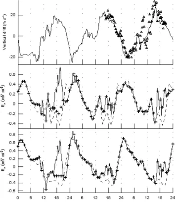
The time variations of the zonal electric field used in the model calculations during 25–27 August 1987 are presented in the middle and bottom panels of Fig. 1. The solid line in the bottom panel of Fig. 1 shows the empirical F -region storm-time equatorial zonal electric field found from the em-pirical model of the vertical drift velocity of Fejer and Scher-liess (1997). For the time periods from 16:30 UT to 21:00 UT on 25 August, this empirical electric field is modified by the use of the comparison between the measured and modeled values of hmF 2 over the Manila sounder (see Sect. 4.1). The resulting storm-time equatorial zonal electric field, EES3 , given by crosses in the bottom panel of Fig. 1, is used in the model calculations at the F -region altitudes over the ge-omagnetic equator. The top panel of Fig. 1 shows the mea-sured (triangles) and modeled (solid line) F -region plasma vertical drift velocity over Jicamarca, which will be dis-cussed in Sect. 4.1.
There are no MU radar vertical drift velocity measure-ments for the studied time period. We take into account that the perpendicular drifts over Arecibo and the MU radar are similar for the same local time (Takami et al., 1996). There-fore, for geomagnetically quiet conditions, it would be possi-ble to use the Arecibo average quiet time zonal electric field, EAQ3 , in model simulations at the F -region altitudes, 29◦ ge-omagnetic latitude, and 201◦ geomagnetic longitude. This zonal electric field is found from Fig. 2 of Fejer (1993) and is shown in the middle panel of Fig. 1 (dashed line). To find the disturbed zonal electric field, EAS3 , at the F -region altitudes, 29◦geomagnetic latitude, and 201◦geomagnetic longitude, we find the difference, 1E3, between the disturbed (crosses in the bottom panel of Fig. 1) and geomagnetically quiet zonal electric fields over the geomagnetic equator. The F -region geomagnetically quiet equatorial zonal electric field is found from the empirical model of the vertical drift ve-locity of Scherliess and Fejer (1999) and is shown by the dashed line in the bottom panel of Fig. 1. In the absence of measurements and an empirical model of a storm-time zonal electric field for the studied time period at geomagnetic lat-itudes close to 29◦, we suggest that the studied storm-time variations in the zonal electric field at the F -region altitudes are the same at the geomagnetic equator and at the geomag-netic latitude of 29◦, i.e. EAS3 =EAQ3 +1E3. The value of EAS3 found is shown by crosses in the middle panel of Fig. 1.
Equations (1)–(3) determine the trajectory of the iono-spheric plasma perpendicular to magnetic field lines and the moving coordinate system. It follows from Eq. (1) that time variations of U caused by the existence of the zonal elec-tric field are determined by time variations of Eeff3 given by Eq. (2). We have to take into account Eq. (3), which shows that Eeff3 is not changed along magnetic field lines. The
equa-Fig. 1. The bottom and middle panels show diurnal variations of the
zonal electric field during 25–27 August 1987. The solid line in the bottom panel shows the F -region storm-time equatorial zonal elec-tric field found from the empirical model of Fejer and Scherliess (1997), while the F -region geomagnetically quiet equatorial zonal electric field found from the empirical model of Scherliess and Fe-jer (1999) is presented by the dashed line in the bottom panel. For the time periods from 16:30 UT to 21:00 UT on 25 August, the empirical electric field, given by the solid line in the bottom panel, is modified by use of the comparison between the measured and modeled values of hmF 2 over the Manila sounder (see Sect. 4.1). The resulting storm-time equatorial zonal electric field, EES3 , given by crosses in the bottom panel of Fig. 1, is used in the model cal-culations at the F -region altitudes over the geomagnetic equator. The average quiet time value of the zonal electric field at the F -region altitudes over Arecibo (dashed line in the middle panel) is found from Fejer (1993). To find the disturbed zonal electric field, EAS3 , at the F -region altitudes, 29◦geomagnetic latitude, and 201◦ geomagnetic longitude, we find the difference, 1E3, between the disturbed (crosses in the bottom panel) and geomagnetically quiet (dashed line in the bottom panel) zonal electric field. We suggest that the studied storm-time variations in the zonal electric field at the F -region altitudes are the same at the geomagnetic equator and at 29◦geomagnetic latitude, i.e. EAS3 =EAQ3 + 1E3. The EAS3 used is shown by crosses in the middle panel. The F -region plasma ver-tical drift velocity, measured by the Jicamarca, radar from 16:31 UT on 26 August 1987, to 20:45 UT on 27 August 1987, is displayed by triangles in the top panel, while the F -region plasma vertical drift velocity over Jicamarca calculated by the empirical model of Fejer and Scherliess (1997) for the time period of 25–27 August 1987 is shown by the solid line in the top panel.
Fig. 2. The variation in the AE index (top panel), the Dst index (middle panel), and Kpindex (bottom panel) during 25–27 August 1987. The SSC onset of the geomagnetic storm is shown by the arrow in the bottom panel.
torial and Arecibo values of the storm-time zonal electric field are used to find the equatorial and Arecibo values of Eeff3 from Eqs. (2) and (3). The equatorial value of Eeff3 is used for magnetic field lines with an apex altitude, hap=Req-RE, less than 600 km, where Req is the equatorial radial distance of the magnetic field line from the Earth’s center and REis the Earth’s radius. The Arecibo value of Eeff3 is used if the apex altitude is greater than 2126 km. A linear interpolation of the equatorial and Arecibo values of Eeff3 is employed at interme-diate apex altitudes.
The model calculates the values of Ni, Ne, Ti, and Te in the fixed nodes of the fixed volume grid. This Eulerian com-putational grid consists of a distribution of the dipole mag-netic field lines in the ionosphere and plasmasphere. One hundred dipole magnetic field lines are used in the model for each fixed value of 3. The number of the fixed nodes taken along each magnetic field line is 191. For each fixed value of 3, the region of study is a (q, U) plane, which is bounded by two dipole magnetic field lines. The low boundary mag-netic field line has hap=150 km. The upper boundary mag-netic field line has hap=4491 km and intersects the Earth’s surface at two middle-latitude geomagnetic latitudes: ±40◦. The computational grid dipole magnetic field lines are dis-tributed between these two boundary lines. They have the interval, 1hap, of 20 km between hap of the low boundary
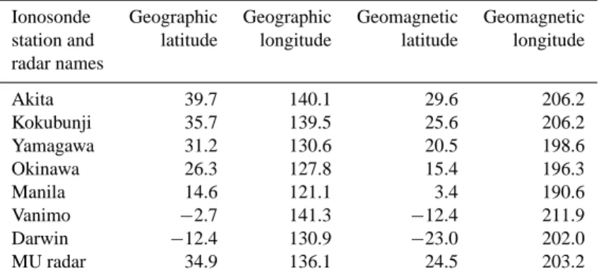
Table 1. Ionosonde station and radar names and locations.
Ionosonde Geographic Geographic Geomagnetic Geomagnetic station and latitude longitude latitude longitude radar names Akita 39.7 140.1 29.6 206.2 Kokubunji 35.7 139.5 25.6 206.2 Yamagawa 31.2 130.6 20.5 198.6 Okinawa 26.3 127.8 15.4 196.3 Manila 14.6 121.1 3.4 190.6 Vanimo −2.7 141.3 −12.4 211.9 Darwin −12.4 130.9 −23.0 202.0 MU radar 34.9 136.1 24.5 203.2
line and hp of the nearest computational grid dipole mag-netic field line. The value of 1hap is increased from 20 km to 45 km linearly as we go from the low computational grid boundary line to the upper computational grid dipole mag-netic field line. We expect our finite-difference algorithm, which is described below, to yield approximations to Ni, Ne, Ti, and Te in the ionosphere and plasmasphere at discrete times t=0, 1t, 21t,... with the time step 1t=10 min. The model starts at 05:14 UT on 23 August. This UT corresponds to 14:00 solar local time, SLT, at the geomagnetic equator and 201◦geomagnetic longitude (SLT=UT+ψ /15, where ψ is the geographic latitude). The model is run from 05:14 UT on 23 August 1987 to 24:00 UT on 24 August 1987 before model results are used.
3 Solar geophysical conditions and data
The storm period under study occurred at solar minimum when the 10.7 cm solar flux was between 85 and 90 dur-ing 25–27 August 1987, and the 3-month average of the 10.7 cm solar flux was 87. In Fig. 2 starting from the bottom panel, the geomagnetic activity indexes Kp, Dst, and AE, are plotted versus universal time, taken by Internet from the database of the National Geophysical Data Center (Boulder, Colorado).
Intense storms have minimum values of Dst≤−100 nT (Gonzalez and Tsurutani, 1987), while the studied storm has the minimum value of Dst=−97 nT at 21:00 UT–22:00 UT on 25 August 1987 with the following recovery phase of the geomagnetic storm. Thus, this storm can be classified as a moderate storm which is very close to an intense storm. The Dst index remained at less than −50 nT up to 09:00 UT on 26 August while the AE index remained perturbed until 21:00 UT on 27 August. The SSC onset of the geomagnetic storm was at 06:58 UT on 25 August and is shown by the arrow in the bottom panel of Fig. 2. The Kpindex reached its maximum value of 60at 12:00 UT–15:00 UT on 25
Au-gust 1987 and at 03:00 UT–06:00 UT on 26 AuAu-gust 1987. The studied storm-time period was preceded by fairly quiet conditions when the value of the geomagnetic Kpindex was
between 0 and 30for most of the time period of 18–24
Au-gust 1987, except between 09:00 UT and 15:00 UT on 24 August when the magnitude of Kpwas 4−.
The middle and upper atmosphere (MU) radar at Shi-garaki, which is located at the geomagnetic latitude of 24.5◦ and the geomagnetic longitude of 203.2◦, operated from 16:00 LT on 25 August to 14:00 LT on 27 August. The capa-bilities of the radar for incoherent scatter observations have been described and compared with those of other incoherent scatter radars by Sato et al. (1989) and Fukao et al. (1990). Rishbeth and Fukao (1995) reviewed the MU radar studies of the ionosphere and thermosphere. The data that we use in this work are the measured time variations of altitude profiles of the electron density and temperature, and the ion temper-ature between 200 km and 600 km over the MU radar.
We use hourly critical frequencies, f of 2 and f oE, of the F2 and E-layers, and maximum usable frequency parame-ter, M(3000)F 2, data from the Akita, Kokubunji, Yamagawa, Okinawa, Manila, Vanimo, and Darwin ionospheric sounder stations available at the Ionospheric Digital Database of the National Geophysical Data Center, Boulder, Colorado. The locations of these ionospheric sounder stations and the loca-tion of the MU radar are shown in Table 1. The values of the peak density, N mF 2, of the F 2 layer are related to the critical frequency f of 2 as N mF 2=1.24·1010f of22, where the unit of N mF 2 is m−3, the unit of f of 2 is MHz. In the absence of adequate hmF 2 data, we use the relation between hmF2 and the values of M(3000)F 2, f of 2, and f oE rec-ommended by Dudeney (1983) from the comparison of dif-ferent approaches as hmF 2=1490/[M(3000)F 2+1M]−176, where 1M=0.253/(f of 2/f oE−1.215)−0.012. There are no f oEdata in the Ionospheric Digital Database for the 25–27 August 1987 time period for the Manila ionosonde station, and we are forced to use 1M=0, i.e. the hmF 2 formula of Shimazaki (1955) is used for the Manila ionosonde station data. The sounders and the MU radar are within ±11◦ ge-omagnetic longitude of one another. As a result, the model simulations are carried out in the plane of 201◦geomagnetic longitude to compare the model results with the MU radar and sounder measurements.
4 Results
4.1 Zonal electric field corrections from the observed vari-ations in hmF 2
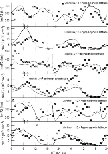
The measured (squares) and calculated (lines) N mF 2 (bot-tom panel) and hmF 2 (top panel) are displayed in Fig. 3 for the 25–26 August 1987 time period above the Vanimo (two bottom panels), Manila (two middle panels), and Okinawa (two top panels) ionosonde stations. The solid lines in Fig. 3 show the calculated N mF 2 and hmF 2 over Manila using the corrected storm-time (crosses in the bottom and middle pan-els of Fig. 1), while the dotted lines in Fig. 3 are N mF 2 and hmF2 from the model with an uncorrected (solid lines in the bottom and middle panels of Fig. 1) zonal electric field. The dashed lines will be explained later in this section. The orig-inal HWW90 wind and NRLMSISE-00 neutral temperature and densities are used in the model calculations.
There are no f oE data for the 25–27 August 1987 time period for the Manila ionosonde station, and we believe that hmF2=1490/M(3000)F 2 over Manila (see Sect. 3). It means that the real values of hmF 2 are less than those shown in the middle panel of Fig. 3 by squares. As a result, if the modeled hmF2 is less than the measured hmF 2, then we cannot de-rive conclusions about errors of the model calculations. For example, there is the disagreement between the measured and modeled hmF 2 over Manila from about 01:00 UT to about 09:00 UT on 25 August. However, we have no right to correct the model input parameters in order for the measured and modeled hmF 2 to agree, because this disagreement (or a part of this disagreement) can be explained by errors in hmF2 found only from the M(3000)F 2 measurements.
The comparison between the measured hmF 2 (squares) and the calculated results, shown by the dotted lines in Fig. 3, clearly indicates that there is a disagreement between the measured and modeled hmF 2 from about 17:00 UT to about 21:00 UT on 25 August, if the equatorial upward E×B drift given by Fejer and Scherliess (1997) is used. As was pointed out above, the measured hmF 2 are less than those shown in the middle panel of Fig. 3 by squares. On the other hand, the measured hmF 2 is less than the calculated hmF 2 over Manila, and we conclude that this disagreement is explained by errors of the model calculations. The model simulations show that changes in the NRLMSISE-00 neutral tempera-ture and densities do not lead to considerable variations in hmF2 and cannot bring the measured and modeled hmF 2 into agreement. By comparing the measured and calculated hmF2 over Manila, we found that the required equatorial upward E×B drift is weaker during the time period from 16:30 UT to 21:00 UT on 25 August than that given by Fejer and Scherliess (1997). The use of the corrected storm-time model equatorial zonal electric field found, shown by crosses in Fig. 1, brings into agreement the measured (squares) and modeled (solid lines) hmF 2 shown in Fig. 3.
The weakening of the zonal electric field from 16:30 UT to 21:00 UT on 25 August causes a noticeable decrease in hmF2 over Manila. The equatorial plasma drift model of
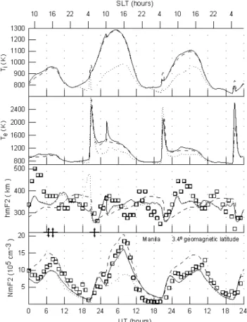
Fig. 3. Observed (squares) and calculated (lines) N mF 2 and hmF 2
during 25–26 August 1987 over the Vanimo (two bottom panels), Manila (two middle panels), and Okinawa (two top panels), The solid lines show the calculated N mF 2 and hmF 2 using the storm-time corrected (crosses in the bottom and middle panels of Fig. 1) zonal electric field, while the dotted lines are N mF 2 and hmF 2 from the model with the uncorrected (solid lines in the bottom and middle panels of Fig. 1) zonal electric field. To produce the model results shown by the dashed lines, the storm-time corrected zonal electric field shown by crosses in the middle and bottom panels of Fig. 1 was divided by a factor of 10 at all the studied geomag-netic latitudes from 02:00 UT to 10:00 UT on 26 August 1987. The original HWW90 wind and NRLMSISE-00 neutral tempera-ture and densities are used in the model calculations. The start times of the sudden commencement (06:58 UT on 25 August), main phase (08:00 UT on 25 August) and recovery phase (22:00 UT on 25 Au-gust) of the geomagnetic storm are indicated by the arrows.
Fejer and Scherliess (1997) does not reproduce this weaken-ing in the zonal electric field which follows from the Manila ionosonde station measurements, because this plasma drift model produces only the averaged vertical drift and this ver-tical drift, can differ from the verver-tical drift for the studied ge-omagnetically disturbed time period. This conclusion is sup-ported by the top panel of Fig. 1, where triangles display the F-region plasma vertical drift velocity measured by the Jica-marca radar from 16:31 UT on 26 August 1987 to 20:45 UT on 27 August 1987, while the F -region plasma vertical drift
velocity over Jicamarca, given by the empirical model of Fe-jer and Scherliess (1997) for the time period of 25–27 August 1987, is shown by the solid line. We conclude from the top panel of Fig. 1 that the measured drift is very variable, and the difference between the empirical model drift velocity and the measured drift velocity during some short time periods on 27 August is comparable to the magnitude of the above-mentioned weakening in the electric field on 25 August.
If E3>0, then a decrease in E3leads to a slower plasma motion from low to high geomagnetic latitudes perpendic-ular to B, causing an increase in N mF 2 and a decrease in hmF2 close to the geomagnetic equator, i.e. it is possible that the disagreement between the measured and modeled N mF 2 over Manila on 26 August (see middle panel of Fig. 3) could be eliminated by a weakening of E3on 26 August in com-parison with that shown by crosses in the middle and bottom panels of Fig. 1. To test this hypothesis, the value of E3 shown by crosses in the middle and bottom panels of Fig. 1 was divided by a factor of 10 at all the studied geomagnetic latitudes from 02:00 UT to 10:00 UT on 26 August. It fol-lows from the model results shown by dashed lines in Fig. 3 that this weakening in E3causes an increase in N mF 2 from about 02:00 UT to about 11:00 UT and a decrease in hmF 2 from about 02:00 UT to about 22:00 UT on 26 August over Manila. However, only a small part of the disagreement be-tween the measured and modeled N mF 2 over Manila can be explained by this reduction in E3. Furthermore, the sug-gested weakening in E3 brings the measured and modeled hmF2 into disagreement over Vanimo and Okinawa on 26 August and worsens the agreement between the measured and modeled hmF 2 over Manila from about 03:00 UT to 07:00 UT and from about 13:00 UT to about 15:00 UT on 26 August. As a result, we have no arguments to correct E3from the comparison between the measured and modeled hmF2 and N mF 2 on 26 August. We show in Sect. 4.2 that the model/data discrepancies over Manila arise due to an in-ability of the NRLMSISE-00 model to accurately predict the thermospheric response to the studied time period in the up-per atmosphere.
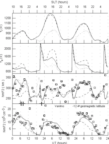
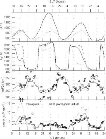
4.2 Diurnal variations of N mF 2, hmF 2, Teand Ti The measured (squares) and calculated (lines) N mF 2 and hmF2 are displayed in the two lower panels of Figs. 4–9 for the 25–27 August 1987 time period above the Darwin (Fig. 4), Vanimo (Fig. 5), Manila (Fig. 6), Okinawa (Fig. 7), Yamagawa (Fig. 8), and Akita (Fig. 9) ionosonde stations, while the modeled electron and O+ion temperatures at the F2-region main peak altitude above the ionosonde stations are presented in the two upper panels of these figures. Fig-ure 10 shows the measFig-ured (crosses) and calculated (lines) N mF2 (bottom panel) and electron (middle panel) and O+ ion (top panel) temperatures at hmF 2 above the MU radar. Squares in the two lower panels of Fig. 10 show the mea-sured N mF 2 and hmF 2 during 25–27 August 1987 above the Kokubunji ionosonde station. The latitude and longitude location of the Kokubunji sounder is very close to that of the
MU radar and the calculated hmF 2, Ne, Te, and Ti above this sounder are practically the same as those in Fig. 10. The results obtained from the model of the ionosphere and plas-masphere using the combination of Eeff3 based on the uncor-rected zonal disturbed electric field (given by the solid lines in the bottom and middle panel of Fig. 1), the NRLMSISE-00 neutral temperature and densities, and the HWW90 wind as the input model parameters are shown by the dotted lines in Figs. 4–10. The solid lines in Figs. 4–10 show the results given by the model with the corrected zonal electric field (given by crosses in the bottom and middle panel of Fig. 1), the corrected NRLMSISE-00 neutral temperature and densi-ties, and the corrected neutral HWW90 wind. Dashed lines in Figs. 4–10 show the results from the model with the same corrections of the NRLMSISE-00 [O] and meridional neutral HWW90 wind as for solid lines and when the value of Eeff3 used in producing results shown by solid lines (based on the corrected zonal electric field given by crosses in the bottom and middle panel of Fig. 1) was divided by a factor of 10 at all the studied geomagnetic latitudes. The NRLMSISE-00 and HWW90 model corrections will be explained below in this section.
It follows from Figs. 4–10 that we are not capable of mak-ing the measured (squares and crosses) and modeled (dotted lines) N mF 2, hmF 2, Te, and Tiagree if the NRLMSISE-00 neutral temperature and densities, the HWW90 wind, the un-corrected Eeff3 (based on the zonal electric field given by the solid lines in the bottom and middle panel of Fig. 1) are used as the input model parameters. A part of these disagreements between the measured and modeled Ne, Te, and Ti is prob-ably due to inaccuracies in the model inputs, such as a pos-sible inability of the NRLMSIS-00 neutral temperature and densities model, the HWW90 wind model, and the empirical electric field model of Fejer and Scherliess (1997) to accu-rately predict the neutral densities, temperature, wind com-ponents, and zonal electric field for the studied period. These models can be corrected for the studied time period from the comparisons between the measured and modeled Ne, Te, and Ti.
By comparing the dotted lines and crosses in the top panel of Fig. 10, it is seen that the measured ion temperature is higher than the calculated one. It follows from Fig. 10 that there is an agreement between the measured and mod-eled electron temperature at hmF 2 over the MU radar from 16:00 UT on 25 August 1987 to 11:00 UT on 26 August 1987. As a result, we can infer that the disagreement between the measured and modeled ion temperature is caused by inac-curacies in the NRLMSISE-00 model prediction of the neu-tral temperature, Tn, for the studied geomagnetic storm-time period. To overcome the disagreement between the measured and modeled ion temperature, we multiply the value of Tnby the correction factor, C, which is determined as
C =1.2 + 0.2·sin[(UT−21)·π/12] from
15 : 00 UT on 25 August to 15 : 00 UT on 26 August, C =1.1 + 0.1·sin[(UT−21)·π/12] from
15 : 00 UT on 26 August to 15 : 00 UT on 27 August, (4)
Fig. 4. Observed (squares) and calculated (lines) N mF 2 and hmF 2
(two lower panels), and electron and O+ion temperatures (two up-per panels) at the F 2-region main peak altitude above the Darwin ionosonde station during 25–27 August 1987. SLT is the solar lo-cal time at the Darwin ionosonde station. The results obtained from the model of the ionosphere and plasmasphere, using Eeff3 based on the uncorrected zonal electric field, given by the solid lines in Fig. 1, the NRLMSISE-00 neutral temperature and densities, and the HWW90 wind as the input model parameters, are shown by dot-ted lines. Solid lines show the results obtained from the model of the ionosphere and plasmasphere using the combinations of Eeff3 based on the corrected zonal electric field given by crosses in Fig. 1, the corrected NRLMSISE-00 neutral temperature and densities, and the corrected meridional HWW90 wind. Dashed lines show the results from the model with the same corrections of the NRLMSISE-00 [O] and meridional HWW90 wind as for solid lines and when the value of Eeff3 used in producing results shown by solid lines (based on the corrected zonal electric field given by crosses in the bottom and middle panel of Fig. 1) was divided by a factor of 10 at all the studied geomagnetic latitudes during the studied time period. The start times of the sudden commencement (06:58 UT on 25 August), main phase (08:00 UT on 25 August) and recovery phase (22:00 UT on 25 August) of the geomagnetic storm are indicated by the arrows.
where the unit of UT is hour. As was pointed out before, we expect that the NRLMSISE-00 neutral model has some in-adequacies in predicting the number densities with accuracy, and we have to change the number densities by correction factors at all altitudes to bring the modeled electron densities into agreement with the measurements. As a result of the
Fig. 5. From bottom to top, observed (squares) and calculated
(lines) of N mF 2, hmF 2, electron temperatures and O+ion tem-peratures at the F 2-region main peak altitude above the Vanimo ionosonde station during 25–27 August 1987. SLT is the solar local time at the Vanimo ionosonde station. The start times of the sudden commencement (06:58 UT on 25 August), main phase (08:00 UT on 25 August) and recovery phase (22:00 UT on 25 August) of the geomagnetic storm are indicated by the arrows. The curves are the same as in Fig. 4.
comparison between the modeled N mF 2 and N mF 2 mea-sured by the Manila ionosonde station (see Fig. 6), the value of [O] was increased by a factor of 2 in the 0–5◦ geomag-netic latitude range of the Northern Hemisphere at all alti-tudes from 02:00 UT to 08:00 UT on 26 August. During this time period, the [O] correction factor varies linearly from 2 to 1 in the geomagnetic latitude ranges between 5◦and 15◦and between 0◦and −10◦. To bring the measured and modeled electron densities into agreement above the Darwin and Van-imo ionosonde stations, the value of [O] was increased by a factor of 1.5 at the geomagnetic latitudes from −15◦to −40◦ at all altitudes from 23:00 UT on 25 August to 02:00 UT on 26 August. To make the measured and modeled N mF 2 agree over the Okinawa, Yamagawa, Kokubunji, and Akita ionosonde stations, the model [O] was decreased by a fac-tor of 1.5 at the geomagnetic latitudes from 15◦ to 40◦ at all altitudes from 22:00 UT on 24 August to 09:00 UT on 25 August, while the model [N2] and [O2] were increased
Fig. 6. From bottom to top, observed (squares) and calculated
(lines) of N mF 2, hmF 2, electron temperatures and O+ion tem-peratures at the F 2-region main peak altitude above the Manila ionosonde station during 25–27 August 1987. SLT is the solar local time at the Manila ionosonde station. The start times of the sudden commencement (06:58 UT on 25 August), main phase (08:00 UT on 25 August) and recovery phase (22:00 UT on 25 August) of the geomagnetic storm are indicated by the arrows. The curves are the same as in Fig. 4.
at all altitudes from 02:00 UT to 08:00 UT on 26 August. During these time periods, a linear variation in the [O] cor-rection factor from 1.5 to 1 is assumed in the geomagnetic latitude range between −15◦and −10◦and between 15◦and 10◦, respectively, while a linear variation in the [N2] and [O2]
correction factor from 2 to 1 is assumed in the geomagnetic latitude range between 15◦and 5◦.
Variations in hmF 2 are predominantly determined by variations in the thermospheric wind at the ionosonde sta-tions, such as Akita, Kokubunji, and Darwin and over the MU radar, which locations that are far enough from the geomagnetic equator (Rishbeth, 2000; Souza et al., 2000; Pincheira et al., 2002; Pavlov, 2003; Pavlov et al., 2004), i.e. effects of the E×B plasma drift on hmF 2 and N mF 2 over these sounders and over the MU radar are much less than those caused by the plasma drift due to the neutral wind. The HWW90 wind velocities are known to differ from ob-servations (Titheridge, 1995; Kawamura et al., 2000; Em-mert et al., 2001; Fejer et al., 2002). To bring the modeled
Fig. 7. From bottom to top, observed (squares) and calculated
(lines) of N mF 2, hmF 2, electron temperatures and O+ion tem-peratures at the F 2-region main peak altitude above the Okinawa ionosonde station during 25–27 August 1987. SLT is the solar local time at the Okinawa ionosonde station. The start times of the sudden commencement (06:58 UT on 25 August), main phase (08:00 UT on 25 August) and recovery phase (22:00 UT on 25 August) of the geomagnetic storm are indicated by the arrows. The curves are the same as in Fig. 4.
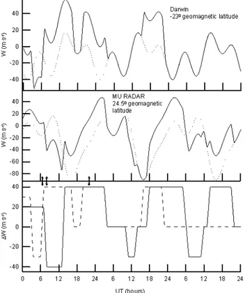
and measured hmF 2 and N mF 2 into reasonable agreement over the Akita, Kokubunji, and Darwin sounders and over the MU radar, the meridional neutral wind, W, taken from the HWW90 wind model, is changed to W+1W. The val-ues of 1W, shown in the low panel of Fig. 11, are used in the Northern Hemisphere above the geomagnetic latitude of 24◦(solid line) and in the Southern Hemisphere below the geomagnetic latitude of −24◦(dashed line), while 1W=0 at the geomagnetic equator. A square interpolation of 1W is employed between −24◦and 0◦and between 24◦and 0◦ ge-omagnetic latitude.
To give an example of changes in the meridional neu-tral wind due to 1W, the diurnal variations of the mod-eled meridional uncorrected HWW90 (dotted lines) and cor-rected (solid lines) neutral winds during 25–27 August 1987 at 300 km are shown in the middle and top panels over the MU radar and over the Darwin ionosonde station, respec-tively. We conclude that the storm-time meridional wind ve-locity has non-regular variations, in agreement with the early
Fig. 8. From bottom to top, observed (squares) and calculated
(lines) of N mF 2, hmF 2, electron temperatures and O+ion tem-peratures at the F 2-region main peak altitude above the Yamagawa ionosonde station during 25–27 August 1987. SLT is the solar lo-cal time at the Yamagawa ionosonde station. The start times of the sudden commencement (06:58 UT on 25 August), main phase (08:00 UT on 25 August) and recovery phase (22:00 UT on 25 Au-gust) of the geomagnetic storm are indicated by the arrows. The curves are the same as in Fig. 4.
conclusions of Kawamura (2003), and the magnitude of the storm-time meridional wind shown by the solid line in the middle panel of Fig. 11 is comparable with that observed by the MU radar during disturbed conditions of 23 March–2 April 2001 studied by Kawamura (2003).
The solid lines in Figs. 4–10 show the results obtained from the model of the ionosphere and plasmasphere using the corrected NRLMSISE-00 neutral temperature and densities, the corrected meridional HWW90 wind, and the corrected zonal electric field. We conclude that the use of the corrected [O], [N2], [O2], Tn, W, and E3brings the measured and mod-eled N mF 2, hmF 2, Te, and Ti into reasonable agreement although there are some quantitative differences.
One can see from Fig. 6 that the NRLMSISE-00 model with the modified [O] improves the agreement with the mea-sured N mF 2 over the Manila ionosonde station. On the other hand, the NRLMSISE-00 model can have some inad-equacies in predicting the actual [N2] and [O2] with
accu-racy. However, to reach approximately the same agreement between the measured and modeled N mF 2 over the Manila
Fig. 9. From bottom to top, observed (squares) and calculated
(lines) of N mF 2, hmF 2, electron temperatures and O+ion tem-peratures at the F 2-region main peak altitude above the Akita ionosonde station during 19–21 March 1988. SLT is the solar local time at the Akita ionosonde station. The start times of the sudden commencement (06:58 UT on 25 August), main phase (08:00 UT on 25 August) and recovery phase (22:00 UT on 25 August) of the geomagnetic storm are indicated by the arrows. The curves are the same as in Fig. 4.
ionosonde station, the values of the NRLMSISE-00 [N2] and
[O2] must be decreased by a factor of 3–3.5 in the 0–5◦
ge-omagnetic latitude range of the Northern Hemisphere from 02:00 UT to 08:00 UT on 26 August at all altitudes without NRLMSISE-00 [O] corrections. If the NRLMSISE-00 [O] Southern Hemisphere correction, which is described above, is not used, then the values of the NRLMSISE-00 [N2] and
[O2] must be decreased by a factor of 2 at the geomagnetic
latitudes from −15◦to −40◦at all altitudes from 23:00 UT on 25 August to 02:00 UT on 26 August, to bring the mea-sured and modeled N mF 2 over the Darwin and Vanimo ionosonde stations into approximately the same agreement. Thus, the comparison between the NRLMSISE-00 [N2] and
[O2] decrease, and the NRLMSISE-00 [O] increase does not
show similarity and consistency in the magnitudes of their effects on N mF 2 at low geomagnetic latitudes. This differ-ence in the response of the calculated N mF 2 to neutral den-sity variations is large enough to provide evidence in favor of changing [O] in comparison with changing [N2] and [O2].
Fig. 10. Observed (crosses) and calculated (lines) N mF 2 and
hmF2 (two lower panels), and electron and O+ion temperatures (two upper panels) at the F 2-region main peak altitude above the MU radar during 25–27 August 1987. SLT is the solar local time at the MU radar. Squares in the two lower panels show the measured
N mF2 and hmF 2 during 25–27 August 1987 above the Kokubunji ionosonde station. The start times of the sudden commencement (06:58 UT on 25 August), main phase (08:00 UT on 25 August) and recovery phase (22:00 UT on 25 August) of the geomagnetic storm are indicated by the arrows. The curves are the same as in Fig. 4 (see first paragraph of Sect. 4.2).
It is well known that N mF 2 is proportional to [O]/[N2]
in the middle-latitude daytime ionosphere (e.g. Rishbeth and Garriot, 1969; Rees, 1989; Lobzin and Pavlov, 2002, and references therein). However, the low-latitude ionosphere is special because of the constraints imposed on electron and ion motions by the magnetic field and by the zonal electric field. In agreement with the results of Pavlov et al. (2004), the model calculations of this work provide an additional evidence that the dependence of N mF 2 on [N2] and [O2]
is weaker than the dependence of N mF 2 on [O] by day at low geomagnetic latitudes, i.e. N mF 2 is not proportional to [O]/[N2] or to [O]/[O2] in the low-latitude daytime
iono-sphere.
To evaluate the relative role of the E×B drift and possible uncertainties in E3in variations of Ne, Ni, Te, and Ti, calcu-lations have been carried out from the model when the value of E3, used in producing results shown by solid lines, was
Fig. 11. Diurnal variations of the meridional HWW90 neutral wind,
W, the correction, 1W, of W during 25–27 August 1987 (when the original value of W is changed to W+1W). The values of 1W shown in the low panel are used in the Northern Hemisphere above the geomagnetic latitude of 24◦ (solid line) and in the Southern Hemisphere below the geomagnetic latitude of −24◦(dashed line), while 1W=0 at the geomagnetic equator. A square interpolation of 1W is employed between −24◦and 0◦and between 24◦and 0◦. The modeled meridional uncorrected HWW90 (dotted lines) and corrected (solid lines) neutral winds at 300 km are shown in the middle and top panels over the MU radar and over the Dar-win ionosonde station, respectively. The meridional HWW90 Dar-wind is directed northward for W>0 and southward for W<0. The start times of the sudden commencement (06:58 UT on 25 August), main phase (08:00 UT on 25 August) and recovery phase (22:00 UT on 25 August) of the geomagnetic storm are indicated by the arrows.
divided by a factor of 10 at all the studied geomagnetic lat-itudes and when the corrections of the NRLMSISE-00 tem-perature and densities and meridional neutral HWW90 wind are the same as for the solid lines in Figs. 4–10. The model results are shown by dashed lines in Figs. 4–10.
During most of the daytime period, the E×B drift lifts the plasma from lower field lines to higher field lines, while during most of the nighttime period, this drift moves ions and electrons from higher to lower magnetic field lines. Si-multaneously, the plasma diffuses along the magnetic field lines. The comparison between the solid and dashed lines in the bottom panel of Fig. 6 shows that, close to the geo-magnetic equator, the N mF 2 enhancement caused by the de-crease in the plasma outflow is stronger than the reduction in N mF2 caused by the increase in the loss rate of O+(4S) ions.
Therefore, the weakening of E3leads to the N mF 2 increase by day over the Manila sounder. The nighttime N mF 2 in-crease is a result of the daytime N mF 2 inin-crease and the decrease in the loss rate of O+(4S) ions due to the hmF 2 increase caused by the weakening of E3.
The complex interplay of the physical processes described above for the Manila sounder determines the variations in N mF2 and hmF 2 caused by the weakening of E3over the other sounders. Figures 4–10 show that the magnitude of the change in N mF 2 caused by the weakening of E3 by a factor of 10 is decreased if the absolute value of the geomag-netic latitude is increased. As an example, above the Akita ionosonde station, this weakening in E3changes N mF 2 and hmF2 up to a factor of 0.85–1.21 and up to the maximum value of 25 km, respectively, while the maximum electron density change is a factor of 0.83–1.5 at 400 km. In agree-ment with the previous study by Pavlov et al. (2004), we conclude that the use of the one-dimensional time dependent model of the ionosphere and plasmasphere, which does not take into account the E×B plasma drift, leads to noticeable errors in the calculated daytime electron density of the F 2 region and a part of the topside ionosphere, even at geomag-netic latitudes of about 25◦−30◦.
The measured hmF 2 presented in Figs. 4–10 show large fluctuations. The possible source of this scatter in hmF 2 is the dependence of hmF 2 on M(3000)F 2 and 1M given by Dudeney (1983) (see Sect. 3), which determines hmF 2 diur-nal variations with errors. Furthermore, there are no f oE measurements over Manila during 25-27 August, i.e. it is suggested that 1M=0. It means that the measured hmF 2 presented in Fig. 6 can be overestimated (Dudeney, 1983). The ionosondes listed in Table 1 are not located at the ge-omagnetic longitudes of 201◦, which is used in the model calculations. This geomagnetic longitude displacement can explain a part of the disagreement between the modeled and measured hmF 2, N mF 2, Te, and Tiin Figs. 4–10. A part of these discrepancies is probably due to the uncertainties in the model inputs, such as a possible inability of the NRLMSIS-00 model to accurately predict the densities and tempera-ture for the studied period at low-latitudes, and uncertainties in the neutral wind, EUV fluxes, chemical rate coefficients, photoionization, photoabsorption and electron impact cross sections for N2, O2, and O.
4.3 Latitude variations in N mF 2 and hmF 2
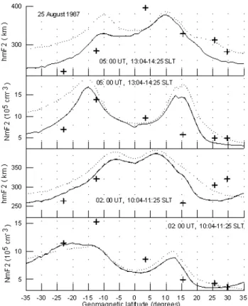
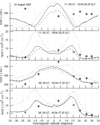
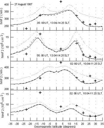
The comparison between the measured (crosses) and mod-eled (lines) N mF 2 and hmF 2 latitude variations is depicted in Figs. 12, 14, and 16 at 02:00 UT (two lower panels) and 05:00 UT (two upper panels) and in Figs. 13, 15, and 17 at 08:00 UT (two lower panels) and 11:00 UT (two upper pan-els) on 25 August (Figs. 12 and 13), 26 August (Figs. 14 and 15), and 27 August (Figs. 16 and 17). The combinations of the model input parameters used in the calculations of the model results, shown by the solid lines, are the same as those for the solid lines in Fig. 4. The dashed lines show the results produced by the model using the combinations of Eeff3 based
Fig. 12. Observed (crosses) and calculated (lines) hmF 2 and
N mF2 at 02:00 UT (two lower panels) and 05:00 UT (two upper panels) on 25 August 1987. The measured hmF 2 and N mF 2 are taken from the ionospheric sounder station listed in Table 1. The solid curves are the same as in Fig. 4. The dotted lines show the re-sults produced by the model, using the combinations of Eeff3 based on the corrected zonal electric field, given by crosses in Fig. 1 (as for the solid lines in Fig. 12), zero neutral wind, and the NRLMSISE-00 neutral densities and temperature with the same corrections of [O] and Tnas for the solid lines in Fig. 12. The dashed lines show the results produced by the model, using the combinations of Eeff3 based on the zonal electric field, given by the dashed lines in Fig. 1, and the HWW90 wind velocities, the NRLMSISE-00 neutral den-sities and temperature with the same corrections of W, [O], [N2],
[O2], and Tnas for the solid lines in Fig. 12.
on the zonal electric field given by the dashed lines in Fig. 1 (i.e. the zonal electric field for geomagnetically quiet condi-tions taken from Fejer (1993) and Scherliess and Fejer (1999) is used), the HWW90 wind velocities, the NRLMSISE-00 neutral densities and temperature with the same corrections of W, [O], [N2], O2], and Tn as for the solid lines. The dot-ted lines show the results produced by the model using the combinations of Eeff3 based on the corrected zonal electric field given by crosses in Fig. 1, zero neutral wind, and the NRLMSISE-00 neutral densities and temperature with the same corrections of the NRLMSISE-00 neutral densities and temperature as for the solid lines.
By comparing the results of calculations presented by the solid lines in Figs. 12, 13, 16, and 17, the similarity of the equatorial anomaly on 25 and 27 August can be seen. If
Fig. 13. Observed (crosses) and calculated (lines) hmF 2 and
N mF2 at 08:00 UT (two lower panels) and 11:00 UT (two upper panels) on 25 August 1987. The measured hmF 2 and N mF 2 are taken from the ionospheric sounder station listed in Table 1. The curves are the same as in Fig. 12.
we compare these solid lines with those in Figs. 14 and 15, we can conclude that the geomagnetic latitude varia-tions in the electron density calculated for 26 August 1987 (the recovery phase of the geomagnetic storm) differ signif-icantly from those calculated for 25 August 1987 (the ini-tial and main phases of the geomagnetic storm and before SSC) and for 27 August 1987 (after the geomagnetic storm). The model calculations presented in Figs. 12, 13, 16, and 17 shows that the equatorial plasma fountain, responsible for the equatorial anomaly formation, undergoes significant in-hibition on 26 August. During 25 and 27 August, the model produces the onset of the equatorial anomaly crest forma-tion near 01:00–01:30 UT and the crests disappear close to 14:00 UT, while a geomagnetic latitude electron density pro-file with two equatorial anomaly crests is distinguished from 01:00 UT to 04:00 UT on 26 August. The principal feature of the equatorial anomaly is the crest-to-trough ratio. The modeled N mF 2 show that the equatorial anomaly effect is most pronounced close to 06:00 UT on 25 and 27 August.
It follows from the model results, shown by the solid lines of Figs. 12, 13, 16, and 17, that the latitude variations of the hmF 2 and N mF 2 are asymmetrical about the geomag-netic equator on 25 and 27 August. As seen from a com-parison between the solid lines of Figs. 14 and 15 and those of Figs. 12, 13, 16, and 17, the north-south asymmetry in
Fig. 14. Observed (crosses) and calculated (lines) hmF 2 and
N mF2 at 02:00 UT (two lower panels) and 05:00 UT (two upper panels) on 26 August 1987. The measured hmF 2 and N mF 2 are taken from the ionospheric sounder station listed in Table 1. The curves are the same as in Fig. 12.
N mF2 is much stronger on 26 August than that on 25 or 27 August. Figure 12 shows that the features of the N mF 2 and hmF 2 daytime latitude variations from 02:00 UT to 05:00 UT on 25 August before SSC are a greater anomaly crest value of N mF 2 in the winter hemisphere and a greater maximum value of hmF 2 in the summer hemisphere. It is seen from the comparison between the corresponding solid lines in Figs. 12 and 14 that there are none of these features in the N mF 2 and hmF 2 from 02:00 UT to 05:00 UT on 26 August at the recovery phase of the geomagnetic storm.
It is clear that the north-south asymmetry in N mF 2 and hmF2 should come about through the asymmetry in neu-tral temperature, densities, and winds relative to the geomag-netic equator. The calculations show that the thermospheric circulation produced by the HWW90 model is not symmet-ric relative to the geomagnetic equator during 25–27 August 1987 (e.g. the middle and top panels of Fig. 11). As can be seen from the comparison between the corresponding solid and dotted lines in Figs. 12–13 and 16–17, the asymmetry in hmF 2 and N mF 2 is decreased if the model uses zero neutral wind. We conclude that the asymmetry in the neu-tral wind given by the HWW90 model determines most of the asymmetry in hmF 2 and N mF 2 between the northern and southern geomagnetic hemispheres on 25 and 27 Au-gust from about 01:00–01:30 UT to about 14:00 UT when
Fig. 15. Observed (crosses) and calculated (lines) hmF 2 and
N mF2 at 08:00 UT (two lower panels) and 11:00 UT (two upper panels) on 26 August 1987. The measured hmF 2 and N mF 2 are taken from the ionospheric sounder station listed in Table 1. The curves are the same as in Fig. 12.
the equatorial anomaly exists in the ionosphere. By com-paring the corresponding solid and dotted lines in Figs. 14 and 15, it is seen that both asymmetries in neutral winds and in neutral temperature and densities relative to the geomag-netic equator are responsible for the north-south asymmetry in N mF 2 and hmF 2 on 26 August.
The differences between the disturbed (crosses in the bot-tom and middle panels of Fig. 1) and quiet (dashed lines in the bottom and middle panels of Fig. 1) zonal electric fields, which are most pronounced from 14:00–16:00 UT to 20:00– 23:00 UT, cause the corresponding noticeable variations in the calculated N mF 2 from about 16:00–17:00 UT to about 20:00–22:00 UT. Taking, for example, the Manila sounder, we found that the effects of disturbances in the zonal elec-tric field lead to the increase in N mF 2 by a factor of 1.2–2.5 from 16:14 UT to 21:04 UT on 25 August, by a factor of 1.2– 3.0 from 17:04 UT to 21:14 UT on 26 August, and by a factor of 1.2–2.5 from 17:54 UT to 20:50 UT on 27 August. On the other hand, the comparison between the corresponding solid and dashed lines in Figs. 12–17 show that the effects of dis-turbances in the zonal electric field on N mF 2 and hmF 2 is hardly distinguished from 02:00 UT to 05:00 UT on 25 Au-gust, from 05:00 UT to 08:00 UT on 26 AuAu-gust, and from 02:00 UT to 11:00 UT on 27 August. We conclude from the model calculations that the storm-time changes in the zonal
Fig. 16. Observed (crosses) and calculated (lines) hmF 2 and
N mF2 at 02:00 UT (two lower panels) and 05:00 UT (two upper panels) on 27 August 1987. The measured hmF 2 and N mF 2 are taken from the ionospheric sounder station listed in Table 1. The curves are the same as in Fig. 12.
electric field are not responsible for the suppression of the equatorial anomaly on 26 August, due to weak differences between the disturbed and quiet zonal electric fields on 26 August.
It can be seen from the comparison of the corresponding solid and dotted lines in Figs. 12–17 that the relative con-tributions of the meridional wind in hmF 2 and N mF 2 lat-itude variations vary with time. We found that close to the geomagnetic equator displacements of hmF 2 and variations in N mF 2, caused by the effects of neutral winds on hmF 2 and N mF 2, are stronger on 26 August than those on 25 and 27 August from 02:00 UT to 11:00 UT. It is interesting to point out that the neutral winds inhibit the development of the equatorial anomaly, leading to a decrease in the crest-to-trough ratio during 25–27 August 1987 (compare the corre-sponding solid and dotted lines in Figs. 12–17).
On the other hand, the model using the combinations of the corrected HWW90 wind velocities, the corrected storm-time zonal electric field, and the original NRLMSISE-00 neutral densities and temperature produces the equatorial anomaly from about 01:00 UT to about 09:00 UT on 26 August. We conclude that the storm-time changes in the neutral densities (due to the correction in the NRLMSISE-00 neutral densities on 26 August described in Sect. 4.2) are also responsible for the equatorial anomaly inhibition on 26 August.
Fig. 17. Observed (crosses) and calculated (lines) hmF 2 and
N mF2 at 08:00 UT (two lower panels) and 11:00 UT (two upper panels) on 27 August 1987. The measured hmF 2 and N mF 2 are taken from the ionospheric sounder station listed in Table 1. The curves are the same as in Fig. 12.
The equatorial hmF 2 and N mF 2 are not expected to be very sensitive to neutral wind variations, since these varia-tions cannot induce significant vertical movaria-tions at the geo-magnetic equator. However, variations in the neutral wind affect electron and ion densities at nonzero geomagnetic lat-itudes, causing corresponding variations in electron and ion densities at all points of these magnetic field lines through diffusion of ions and electrons along the magnetic field lines. The E×B drift of electrons and ions redistribute these changes in electron and ion densities between field lines. As a result, variations in the neutral wind at nonzero geomag-netic latitudes can lead to changes in electron density alti-tude profiles close to the geomagnetic equator, resulting in corresponding variations of equatorial hmF 2 and N mF 2. It is necessary to point out that Ne changes more slowly with altitude close to geomagnetic equator at F -region altitudes and in the topside ionosphere in comparison with altitude changes in Ne at middle geomagnetic latitudes. Therefore, small variations in Ne near hmF 2 can change hmF 2 close to the geomagnetic equator. The neutral wind causes large north-south asymmetries in Ne. As a result, the use of zero neutral wind instead of the corrected HWW90 wind causes strong electron density changes in the Northern and Southern Hemispheres, resulting in N mF 2 and hmF 2 changes shown in Figs. 12–17. This change in W is more pronounced on 26 August in comparison with that on 25 and 27 August (see,
for example, the magnitudes of W shown by the solid lines in the middle and top panels of Fig. 11). As a result, dis-placements of hmF 2 and variations in N mF 2, caused by the effects of neutral winds on hmF 2 and N mF 2, are stronger on 26 August than those on 25 and 27 August.
It is found by Pavlov (2003) and Pavlov et al. (2004) that the daytime magnitude of N mF 2 is reduced up to a maxi-mum factor of 1.44 and 1.16 between −30◦and +30◦of the geomagnetic latitude, due to enhanced vibrational excitation of N2and O2during quiet conditions at high and moderate
solar activities, respectively. We found that, in the plane of the geomagnetic meridian at the geomagnetic longitude of 201◦, the increase in the loss rate of O+(4S) ions, due to the vibrational excited N2and O2, causes the maximum
de-crease in the calculated N mF 2 by a factor of 1.12, 1.26, and 1.13 and the maximum change in the calculated hmF 2 of 4, 11, and 4 km in the low-latitude ionosphere between −30◦ and +30◦of the geomagnetic latitude at low solar activity on 25, 26, and 27 August, respectively. It is interesting to point out that, in this latitude range, the maximum decrease in the calculated electron density, caused by reactions of O+(4S)
ions with vibrationally excited N2and O2, is a factor of 1.10
(1.07), 1.35 (1.22), and 1.15 (1.09) at 250 (300) km altitude on 25, 26, and 27 August, respectively. The average daytime neutral temperature is greater on 26 August than that on 25 August or 27 August, due to the correction factor given by Eq. (4). Figures 4–10 show that the average daytime elec-tron temperature is less on 25 August or 27 August than that on 26 August. As a result, the vibrational temperatures of N2and O2are largest on 26 August, and the resulting effect
of vibrationally excited N2 and O2on the electron density
of the low-latitude ionosphere is largest on 26 August. It is possible to point out that the increase in the O+(4S) loss rate due to vibrationally excited O2is less than that due to
vibrationally excited N2. The difference between the N2
vi-brational temperature and the neutral temperature is less than 167 K, 364 K, and 270 K, and this difference is larger than −184 K, −202 K, and −15 K at hmF 2 between −30◦and +30◦of the geomagnetic latitude on 25, 26, and 27 August, respectively.
4.4 Electron and ion temperature variations
The two upper panels of Figs. 4–10 show the calculated (lines) electron, Te, and ion, Ti, temperatures at the F 2-region main peak altitude for the 25–27 August 1987 time period above the Darwin (Fig. 4), Vanimo (Fig. 5), Manila (Fig. 6), Okinawa (Fig. 7), Yamagawa (Fig. 8), and Akita (Fig. 9) ionosonde stations and above the MU radar (Fig. 10). Crosses in the two top panels of Fig. 10 show the electron and ion temperatures measured by the MU radar at hmF 2 during 25–27 August 1987. If we take into account the accuracy of the MU radar electron and ion temperature measurements (Sato et al., 1989) and uncertainties of model calculations, then we conclude that the electron and ion temperatures ob-served by the MU radar are in reasonable agreement with the model results, shown by the solid lines in the two upper