HAL Id: hal-00316957
https://hal.archives-ouvertes.fr/hal-00316957
Submitted on 1 Jan 2001
HAL is a multi-disciplinary open access
archive for the deposit and dissemination of
sci-entific research documents, whether they are
pub-lished or not. The documents may come from
teaching and research institutions in France or
abroad, or from public or private research centers.
L’archive ouverte pluridisciplinaire HAL, est
destinée au dépôt et à la diffusion de documents
scientifiques de niveau recherche, publiés ou non,
émanant des établissements d’enseignement et de
recherche français ou étrangers, des laboratoires
publics ou privés.
high-latitude plasma sheet boundary at midnight
J. M. Quinn, G. Paschmann, R. B. Torbert, H. Vaith, C. E. Mcilwain, G.
Haerendel, O. Bauer, T. M. Bauer, W. Baumjohann, W. Fillius, et al.
To cite this version:
J. M. Quinn, G. Paschmann, R. B. Torbert, H. Vaith, C. E. Mcilwain, et al.. Cluster EDI convection
measurements across the high-latitude plasma sheet boundary at midnight. Annales Geophysicae,
European Geosciences Union, 2001, 19 (10/12), pp.1669-1681. �hal-00316957�
Geophysicae
Cluster EDI convection measurements across the high-latitude
plasma sheet boundary at midnight
J. M. Quinn1, G. Paschmann2, R. B. Torbert1, H. Vaith2, C. E. McIlwain3, G. Haerendel4, O. Bauer2, T. M. Bauer2, W. Baumjohann5, W. Fillius3, M. Foerster2, S. Frey2, E. Georgescu2, S. S. Kerr3, C. A. Kletzing6, H. Matsui1, P. Puhl-Quinn2, and E. C. Whipple7
1Space Science Center, Morse Hall University of New Hampshire Durham, NH 03824, USA
2Max-Planck-Institut f¨ur extraterrestrische Physik D-87545 Garching, Germany
3Center for Astrophysics and Space Sciences University of California, San Diego La Jolla, CA 92093, USA
4International University Bremen, 28725 Bremen, Germany
5Space Research Institute, 8042 Graz, Austria
6Department of Physics and Astronomy University of Iowa Iowa City, IO 52242, USA
7Geophysics Program University of Washington Seattle, WA 98195, USA
Received: 17 April 2001 – Revised: 1 July 2001 – Accepted: 6 July 2001
Abstract. We examine two crossings of three Cluster
satel-lites from the polar cap into the high-latitude plasma sheet at midnight local time, using data from the Electron Drift In-strument (EDI). EDI measures the full electron drift velocity in the plane perpendicular to the magnetic field for any field and drift directions. The context of the measured convec-tion velocities is established by their relaconvec-tion to the intense enhancements in 1 keV electrons, also measured by EDI, as the satellites move from the polar cap into the plasma sheet boundary. In both cases presented here, the cross B convec-tion in the polar cap is anti-sunward (toward the nightside plasma sheet) with a small duskward component. As the satellites enter the plasma sheet boundary region, the dawn-dusk convective flow component reverses its sign, and the flow in the meridianal plane (toward the center of the plasma sheet) drops substantially. The relatively stable convection in the polar cap becomes highly variable as the PSBL is en-countered. The timing and sequence of the boundary cross-ings by the Cluster satellites are consistent with a relatively static structure on a time scale of the few minutes in satel-lite separations. In one of the two events, the plasma sheet boundary has a spatially separate structure that is crossed by the satellites before entering the plasma sheet.
Key words. Magnetospheric physics (electric fields;
mag-netopause, cusp and boundary layers; instruments and tech-niques)
1 Introduction
A primary objective of the Cluster mission is the investiga-tion of boundary structures using multi-point measurements to deconvolve spatial and temporal variations. The
bound-Correspondence to: J. M. Quinn (jack.quinn@unh.edu)
ary between the high-latitude plasma sheet and the polar cap/tail lobe is one such region to be explored by Cluster with
north-south traversals at distances of ∼ 7 RE near perigee
and ∼ 20 RE at apogee. In this paper, we present initial
re-sults from two consecutive Cluster perigee passes through the polar cap plasma sheet boundary at midnight, using elec-tron drift velocities and 1 keV elecelec-tron fluxes from the Elec-tron Drift Instrument (EDI).
The high-latitude nightside plasma sheet boundary region is home to a wide range of important processes involved in auroral acceleration, ionospheric outflow, magnetic reconfig-uration, transient convective plasma transport, and electro-magnetic energy transfer. The electric fields and resulting convective flows, together with other related manifestations of the complex physical processes at the plasma sheet bound-ary, have been investigated on several missions (ISSE, S3-3, Interball, Polar), (e.g. Cattell et al., 1982; Eastman et al., 1984; Pederson et al., 1985; Torbert and Mozer, 1978; Sauvaud et al., 1999; Wygant et al., 2000).
Cluster EDI measurements at the plasma sheet boundary region offer multi-point measurements of the electron drift velocities, or equivalently the electric fields, for both compo-nents of the convective drift, for arbitrary orientations of the magnetic field with respect to the spacecraft spin axis. We present below a first look at EDI measurements in the night-side high-latitude plasma sheet boundary region. Results on the dayside are described in a companion paper (Paschmann et al., 2001, this issue).
2 Technique
The Electron Drift Instrument measures the electron drift
ve-locity, Vd, by detecting the displacement of two weak beams
of test electrons. The technique intrinsically measures both components of drift in the plane perpendicular to the
ambi-ent magnetic field, B, for arbitrary oriambi-entations of Vdand B
with respect to the spacecraft spin axis.
The physical basis of the measurement is the perturbation of the electron’s gyro orbit from the circular trajectory that it would follow in the absence of a drift. This perturbation can be measured in two different ways in order to determine the magnitude and direction of the electron drift velocity. The first method uses the fact that the perturbed trajectory of an electron beam, fired perpendicular to the ambient magnetic field, returns to the spacecraft after one or more gyro orbits
only when fired in unique directions. By finding these
di-rections, one can deduce the drift velocity using a “triangu-lation” technique. The second method measures the times-of-flight for the electron beams to return to the spacecraft, which in the presence of a drift, differ from the gyro period
by amounts that are proportional to ±Vd. The two
tech-niques are complementary in that triangulation is most ac-curate for small-to-moderate drifts, while the time-of-flight is better for moderate-to-large drifts. Cluster’s time-of-flight measurements are discussed further in the companion paper by Paschmann et al. (2001, this issue). In this paper, we present data using only the triangulation technique.
2.1 EDI triangulation measurement of drift velocity
In a uniform magnetic field with no other forces acting, an electron beam fired in any direction perpendicular to the am-bient magnetic field, B, will execute a circular gyro orbit and return to its starting point. In the presence of a transverse electric field, E (or magnetic gradient), the trajectories are distorted, and the electrons no longer return to their starting position after one gyro period. Instead, all electrons starting at a particular location are displaced by the same amount in one gyro period due to the E × B (or grad–B) drift, regard-less of their original direction of travel. This displacement is independent of beam energy for the E × B drift, and propor-tional to the energy for the grad-B drift. The drift step, d, is defined to be the net displacement during one gyro period,
Tg, due to a drift velocity, Vd(Quinn et al., 1979)
d = VdTg. (1)
A measurement of the drift step, together with the knowledge of the gyro period, is thus sufficient to determine the drift velocity.
The EDI triangulation technique is illustrated conceptually in Fig. 1, which is drawn in the plane perpendicular to B (the
“B⊥ plane”). There are two electron guns, with a detector
(Det) located halfway in between. Red and blue lines rep-resent the electron beams. The electron gyro radius is very large (≥ 1 km) compared to the scale of the figure (∼ 1 m), so the gyro trajectories of the beams appear as straight lines. The magnitude and orientation of the drift step, d, is deter-mined by the ambient fields, as described above. We have drawn d with its head positioned at the detector. By
defi-nition of the drift step, any 90◦pitch-angle electron passing
through the tail end of d will be displaced by the drift ve-locity and will hit the detector exactly one gyro period later.
Gun 2 Gun 1 Det d returning beams d = ( Vdrift) ( Tgyro) B
Fig. 1. Principle of EDI triangulation, projected in the plane perpen-dicular to B. The gyro radius of the beam electrons is much larger than the scale of the figure, so the beams appear as straight lines. The “drift step”, d, is the gyro motion displacement in exactly one gyro period. With the head of the d vector placed at the detector, electron beams successfully aimed at the tail of d will return to the detector after one gyro orbit. The combined firing directions of two guns and the known geometric positions of the guns and detector are sufficient to determine the drift step, and thus the drift velocity, from triangulation.
Therefore, an electron beam aimed so that it passes through the tail of d will return to hit the detector after one gyro orbit. Thus, the tail of d represents a “target”, which if hit, will re-sult in the electrons returning to the detector. Electrons fired in other directions and not passing through the target position will not hit the detector, except for those fired in the opposite direction, which also have a virtual source at the tail of d.
When both guns are aimed in the unique directions that al-low their beams to hit the detector after one gyro orbit, one can determine from triangulation the beam intersection point, which corresponds to the tail of d. Using the known locations of the guns and the detector, one can then calculate the vector
d. Together with the knowledge of the gyro period, this
mea-surement of d determines the drift velocity of the electrons. The Cluster EDI gun-detector configuration necessarily differs from that shown in Fig. 1, but it is geometrically equivalent. (The Cluster geometry, together with the full gyro motion of both electron beams, is illustrated in Fig. 1 of Paschmann et al., 2001, this issue). There are two gun-detector units (GDUs) mounted on opposite sides of the spacecraft, with oppositely directed fields-of-view. Each gun is capable of firing its beam in any direction within a bit more
than a full hemisphere, at polar angles up to 96◦, to an
ac-curacy of better than 1◦. Similarly, each detector is able to
detect electrons coming from any selected direction within
a hemispherical field-of-view for polar angles up to 100◦.
Cluster-EDI 20
Oct. 2000 SC-3
0.5 s Intervals at 10 Minute Spacing
-10 -5 0 5 10 X ⊥ (m) -10 -5 0 5 10 Y ⊥ (m)
Cluster-EDI (HR) Triangulation for 20 Oct 2000 15:50:06.323 ± 0.186"
q = 3 15:50 -10 -5 0 5 10 X ⊥ (m) -10 -5 0 5 10 Y ⊥ (m)
Cluster-EDI (HR) Triangulation for 20 Oct 2000 16:00:01.000 ± 0.250"
q = 3 16:00 -10 -5 0 5 10 X ⊥ (m) -10 -5 0 5 10 Y ⊥ (m)
Cluster-EDI (HR) Triangulation for 20 Oct 2000 16:10:02.500 ± 0.250"
q = 3 16:10 -10 -5 0 5 10 X ⊥ (m) -10 -5 0 5 10 Y ⊥ (m)
Cluster-EDI (HR) Triangulation for 20 Oct 2000 16:20:04.250 ± 0.250"
q = 3
16:20
Fig. 2. Sample EDI triangulation plots for four 0.5 s intervals, spaced 10 min apart. Red and green lines are the firing lines of the two electron guns for those times when the beams were properly aimed to return to the detector. The gun positions (symbols) projected into the plane perpendicular to the magnetic field move on an ellipse as the spacecraft rotates through 1/8 of a spin in each panel. The measured “drift step” is the vector from the beam intersection to the center of the figure.
the opposite side of the spacecraft. Thus, for the purposes of triangulation, the baseline separating a gun from its cor-responding detector is the spacecraft diameter projected into
the B⊥plane. At any instant, one gun fires at a detector that
is displaced from it in the B⊥plane by a baseline b, while the
other gun fires at a detector displaced by –b. Therefore, the Cluster configuration is geometrically identical to that shown in Fig. 1 of this paper, where each of the two guns is sepa-rated from its detector by equal distances in opposite direc-tions. (The triangulation baseline, formed by the projection
of the gun-detector separation vectors in the B⊥plane, varies
with the orientation of the ambient magnetic field and space-craft spin phase.) For the purposes of displaying
triangula-tion data, we will continue to use this picture, i.e. two guns and a single “virtual detector” located halfway in between at a distance of one spacecraft diameter from each gun.
Figure 2 shows sample EDI triangulation data in four, 0.5 s, intervals, separated from each other by 10 min. In each interval, those beam-firing directions that returned to the de-tector are plotted and drawn as straight lines with red and green indicating the beams from the two different guns. The position of the virtual detector is at the center of the pic-ture. As the satellite rotates, the projection of the gun
posi-tions sweep out an ellipse when projected into the B⊥plane.
Shading indicates this ellipse, and the gun firing positions at the time of each return beam (each “hit”) are shown by small
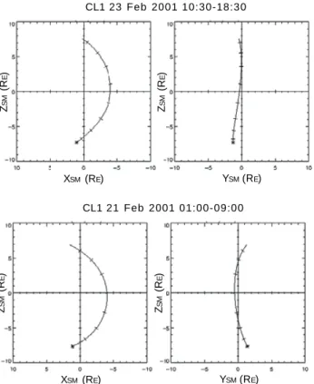
CL1 23 Feb 2001 10:30-18:30 XSM(RE) YSM (RE) Z SM (R E ) Z SM (R E ) CL1 21 Feb 2001 01:00-09:00 XSM(RE) YSM (RE) Z SM (R E ) Z SM (R E )
Fig. 3. Cluster 1 orbit plots in solar magnetospheric coordinates for perigee passes on 23 February (top) and 21 February (bottom) 2001. The Cluster satellites approach perigee through the southern polar cap, pass through the equatorial plane near midnight, and exit to the north. The 8-h orbit plots begin at the asterisk, with tics placed at each UT hour, on the hour.
symbols where the beams intersect the edge of the ellipse. In each of the four time periods, the beams from both guns cross at a well-defined intersection, defining the location of the target. The drift step is simply the vector from this target to the virtual detector at the center of the figure. During this 30-min period from which these samples are taken, the drift
step changes direction by approximately 90◦ and increases
steadily in magnitude.
The ground analysis of the beam firing directions needed to determine the drift steps, and ultimately the drift veloci-ties, uses essentially the same data as displayed in Fig. 2. A fitting procedure identifies the best beam intersection point for all successful beams within a chosen analysis interval, and assigns a chi-squared “quality” to the fit for each inter-val. This analysis is described in the companion paper by Paschmann et al. (2001, this issue). The results presented in this paper use analysis intervals of one-half spin (2 s). How-ever, the analysis can be done over arbitrary intervals, pro-viding that enough beams are present to define a clear inter-section. The limiting time resolution is not fixed, but depends on the rate of successful beam “hits” that are obtained by the onboard tracking algorithm.
2.2 Cluster EDI implementation
The electron beam triangulation technique was first devel-oped by the group at the Max-Planck-Institut f¨ur extrater-restrische Physik (MPE), and flown on the GEOS-2 satellite (Melzner et al., 1978). While the GEOS experiment clearly established the viability of the measurement technique (e.g. Baumjohann et al., 1985), its time resolution was limited to the 6-s spacecraft spin period, and its beam deflection ca-pability restricted operation to a narrow range of magnetic field orientations. The EDI instrument for the Cluster and Equator-S missions was developed to remove these limita-tions as well as to incorporate the time-of-flight technique and other improvements that were necessary to accommo-date the wide range of anticipated magnetic fields, electric fields, and ambient (background) electron fluxes.
Detailed technical descriptions of the EDI instrument are given in several previous publications (Paschmann et al., 1997, 1998, 1999; Vaith et al., 1998), with recent updates discussed by Paschmann et al. (2001, this issue). The key elements for the present paper are the beam firing angles of the guns, the beam recognition by the detector, and the beam acquisition and tracking algorithms which allow for sufficiently frequent “hits” to obtain good triangulation mea-surements. The angles in the triangulation measurement are taken from the gun firing directions, which were calibrated prior to launch over the entire gun solid angle. Since the beam can only return to the spacecraft if it is fired within
ap-proximately 1◦ (the beam width) of the B⊥ plane, we can
check and update these calibrations in orbit by analyzing the distribution of beam hits over the gun solid angle for various magnetic field orientations. On Cluster and Equator-S, we have found that the guns’ ground calibrations perform very well in orbit.
Each EDI gun-detector pair independently acquires and tracks the target by controlling the gun firing directions with a sophisticated, onboard servo algorithm. EDI on Cluster uses beam energies of 1.0 and 0.5 keV to distinguish the ef-fects of E × B drifts, which are independent of energy, and grad-B drifts, which are proportional to energy. In most re-gions, the E × B drift is strongly dominant, and thus the dif-ferences between the 1.0 and 0.5 keV beams are quite small (see, for example, Paschmann et al., 2001, this issue). In this paper, we present only results from 1 keV beams.
The electron beams are amplitude-modulated with one of two pseudo-noise codes: a “long code” with 127 chips, or a “short code” with 15 chips, and the detected counts are processed by a 15-channel correlator. To acquire the target, the beam firing direction is stepped at a constant angular rate
in the B⊥plane until the beam-recognition algorithm records
a hit by analyzing the counts from the different correlator channels. When the beam is detected, the onboard tracking algorithm reverses the angular stepping direction so that the beam is swept repeatedly back and forth across the target direction.
The relevant physical parameters for the EDI triangula-tion technique are the magnetic field and the drift velocity,
Fig. 4. EDI drift velocities for 23 February 2001, for spacecraft 1, 2, and 3, using the standard Cluster color assignments (1 = black; 2 = red; and 3 = green). V X⊥and V Y⊥are velocity components in the plane perpendicular to B with X⊥closest to XGSEand Y⊥closest to YGSE.
Dashed vertical lines mark the satellite encounters with the 1 keV electron boundary (see Fig. 7).
which together determine the magnitude and direction of the drift step. Details of this dependence are given in Quinn et al. (1999) and Paschmann et al. (1999). The accuracy with which one can determine the drift step through triangu-lation depends on several factors, including the knowledge of the beam firing direction and the relative magnitude and orientation of the gun-detector baseline b, projected into the
B⊥plane, with respect to the drift step, d. In general,
tri-angulation is most accurate when the baseline is compara-ble in magnitude to the drift step. However, with firing
an-gles known to 1◦, the drift steps can be measured to better
than 20% over a sufficient dynamic range for many magne-tospheric regions. When drift steps are a few tens of times larger than the baseline, the drift direction is known accu-rately, but the magnitude obtained by triangulation becomes increasingly uncertain. Fortunately, as the triangulation ac-curacy decreases in the large d regime, the time-of-flight technique becomes more accurate (e.g. often in the magne-tosheath), making the two techniques highly complementary.
For extremely small drift steps, the measured magnitude is known to be small, but the direction becomes increasingly uncertain. For the region of space covered in this paper, drift steps in the satellite frame of reference are typically of the order of 1 m, which is ideal for triangulation with baselines on the order of the spacecraft diameter.
A key feature of EDI is that the technique is independent of the orientations of the electric and magnetic fields. The instrument measures both components of the drift velocity
(or equivalently, the electric field) in the B⊥plane, without
regard to the relative orientations of the magnetic field, the spacecraft spin axis, and the drift direction.
We note that in the presence of a sufficiently large elec-tric field parallel to B, the beam would be accelerated along the magnetic field and would not return to the spacecraft. In principle, the detection of a return beam places an upper limit on the parallel electric field. In practice, however, the limit-ing value is very large, and generally does not play a role in
Fig. 5. Drift velocities for the 23 February southern hemisphere crossing from the polar cap into the high-latitude plasma sheet. Same format as Fig. 4. Vertical dashed lines show when the spacecraft encountered the intense 1 keV electron boundary (see Fig. 7).
given beam width and energy, the ratio of Ek/B determines
whether the displacement of the beam by the parallel elec-tric field in one gyro orbit is greater than its dispersion along
the magnetic field. As an example, a 1 keV beam of 1◦
half-width in a 100 nT magnetic field requires a parallel electric field of 10.4 mV/m to displace the beam enough so that it is not detected.
2.3 Ambient electron monitoring
In addition to sensing the return electron beams, the EDI de-tectors make a continuous measurement of ambient electrons at the beam energy of 1.0 or 0.5 keV, and pitch-angles of
approximately 90◦. While these ambient fluxes represent a
source of “background” to the primary EDI beam detection, they also provide a valuable diagnostic of the local plasma regime at relatively high time resolution. In this paper, we present ambient electron measurements at 1 keV only.
During normal operations, the EDI detectors are contin-uously steered perpendicular to the magnetic field in order
to sense the return beam electrons. Depending on whether or not the beam pseudo-noise code is detected by the EDI correlator, the electron counts are identified as either ambi-ent background, or a returning beam. The time resolution of the ambient electron measurements varies with telemetry mode and with the number of samples in which the return beam is successfully detected. For the normal-rate teleme-try data used in this paper, the electron count rate sampling is returned at a rate of 8 samples/s. (In high-rate telemetry, the sampling is 8 times faster). Depending on the onboard beam-tracking duty cycle, the division of these samples be-tween ambient and beam measurements can vary substan-tially, from nearly 100% beam during good tracking, to less than 20%. Assuming that typically 50% of the telemetered electron samples are beams, then the ambient electron data have an average sampling rate of approximately 4 samples/s. The EDI geometric factor and efficiencies vary somewhat with the detector look-direction and, more substantially, with the detector “Optics State” (see Paschmann et al., 1997, for a discussion of the adjustable geometric factor of EDI’s
de-tector optics). The ambient electron data presented here are from a fixed Optics State. As is evident in the data, the effects of the look-direction are negligible compared to the orders-of-magnitude variations in the ambient electrons which are presented below. In future work, a quantitative on-orbit de-termination of the detector geometric factor and efficiencies will enable smaller scale ambient electron features to be re-liably used for detailed timing.
3 Convection measurements at high-latitudes near perigee
We now examine EDI convection velocities in relation to the high-latitude plasma sheet boundary during two consecutive perigee passes of the Cluster spacecraft in February 2001. At this time, the orbit plane was nearly in the noon-midnight meridianal plane, with perigee at approximately midnight. Figure 3 shows the Cluster orbits for the 8-h perigee passes on 23 and 21 February, in solar magnetospheric coordinates. For each pass, we will present an overview of the 8-h period, and then look in detail at the southern hemisphere crossings from the polar cap into the plasma sheet. During the or-bits of this study, EDI was not operated for approximately a 2-h period centered on perigee. However, good measure-ments were made in the regions of the high-latitude plasma sheet boundary and polar cap. In addition, EDI was not op-erated on spacecraft 4 during these orbits, so we present only data from spacecraft 1, 2, and 3. The periods of the Clus-ter perigee passes studied below are geomagnetically quiet
to moderately active. KP is between 1+ and 2+ for the
8-h periods s8-hown on eac8-h orbit. Wide band auroral images from the IMAGE WIC instrument show some substorm ac-tivity before and after the perigee passes, but relatively quiet arcs during the plasma sheet boundary crossings that are an-alyzed in detail below (private communication, Mende and Frey, 2001).
3.1 23 February 2001
Figure 4 shows an overview of EDI drift velocities for the 8-h orbit segment of Fig. 3, for Cluster spacecraft 1 (black), 2 (red), and 3 (green). The data are presented in a magnetic
field oriented coordinate system, X⊥, Y⊥, Z⊥, defined for
each spacecraft as follows:
Z = ±B/B
(sign chosen to have a positive ZGSE component) (2a)
X⊥=YGSE×Z (2b)
Y⊥=Z × X⊥. (2c)
This system is well suited to display E × B (and other) drift velocities that are, by definition, perpendicular to the
magnetic field. The X⊥ component represents drift within
the plane perpendicular to B that is closest to the sunward
direction, while the Y⊥ component is drift transverse to the
Earth-Sun line in the duskward direction. For B parallel to
Fig. 6. Relative positions of spacecraft 1, 2 and 3 at the time of crossing into the intense 1 keV electron population of the southern plasma sheet on 23 February. Positions with respect to spacecraft 1 are represented by dots using the standard color assignments. Three panels show projections in the 3 principle GSE coordinate system planes. The lower right panel is the projection in the plane perpen-dicular to the magnetic field. +X⊥is the direction closest to the Sun in this plane. The spacecraft velocity vector is shown by the solid line, scaled so that 5 km/s corresponds to a value of 1500 on the km scale. The magnetic field unit vector projection is given by the dashed line.
ZGSE, the X⊥, Y⊥coordinates reduce to XGSE, YGSE. For
the remainder of the paper, we refer to the X⊥–Y⊥plane as
the “B⊥plane”.
The top two panels show the drift velocity components in the plane perpendicular to B. The values for spacecraft 2 and 3 are offset for visibility by +10 and −10 km/s, respec-tively, and the zero level for each spacecraft is indicated by the horizontal dashed line. The third and fourth panels show
the magnitude of the velocity and its direction within the B⊥
plane with respect to +X⊥. Each point is the average drift
velocity determined from all return beams in a 1/2 spin. De-tails of the ground analysis process are given by Paschmann et al. (2001, this issue). The velocities are in an “inertial” frame, i.e. the contribution from spacecraft velocity has been subtracted. At the beginning of the interval, from about 10:30 to 12:00 UT, Cluster is moving across the southern polar cap
at a geocentric distance of 6–7.5 RE. During this period,
the V X⊥component shows an “anti-sunward” convection of
about 10 km/s. Although the direction of X⊥varies with the
magnetic field orientation, the flow in the X⊥ direction is
always towards the nightside. During this same period, the
V Y⊥component of flow is smaller, oriented toward dusk at
<5 km/s.
As the satellites approach the plasma sheet (12:00– 12:40 UT), the anti-sunward flow (toward the nightside plasma sheet) and the duskward flow decrease, with both
Fig. 7. EDI 1 keV, 90◦pitch-angle am-bient electron counts for spacecraft 1, 2, and 3, using the same colors as in the other figures. Counts for space-craft 1 and 3 are offset by factors of 25 and 5, respectively. Count levels of 0 and 1 are clipped. Fiducial marks at the strong count intensifications seen by each spacecraft are plotted at 13:12:30, 13:15:25 and 13:18:20 UT.
components becoming more variable as the V X⊥component
reaches zero at about 12:50 UT. The vertical dashed lines at 13:12–13:18 mark the times of entry into the 1 keV electron plasma sheet for each spacecraft, as discussed below in
re-lation to Fig. 7. At this time, the V Y⊥ component of flow
shows a reversal, changing from duskward to dawnward. Following entry into the plasma sheet, the flow velocity variability continues (seen in spacecraft 1) until operations are suspended through the equatorial perigee portion of the orbit. This variability is not fully resolved in the half-spin averaged data shown here.
In the northern hemisphere segment of the orbit, following the data gap at perigee, the flows are again highly variable un-til the satellites exit the plasma sheet at 16:10. At that time,
the consistent anti-sunward flow resumes in the V X⊥
com-ponent. The velocity of this “steady” anti-sunward flow in the northern hemisphere is immediately at ∼ 10 km/s, show-ing little sign of the slower flow transition near the plasma sheet boundary that was seen in the southern hemisphere.
Throughout this interval, the flows seen by the three satel-lites are in good agreement. At the time of the plasma sheet entry, the satellites are separated by distances of the order of 1000 km, and times of about 1–2 min. As expected, the tim-ing differences between the observed features are not readily apparent on the large time scale of Fig. 4.
We now look with higher time resolution at the southern hemisphere crossing from the polar cap into the plasma sheet. Figure 5 shows flow velocities in the same format as before for a 2-h interval containing this crossing. In the spacecraft 1 data, there is a distinct, qualitative change in the character of the velocities near the time of the black dashed line, from relatively smooth to much more variable, with fewer points. There are three contributions to this change. First and most important, the drift velocities are much more variable in the later region than in the preceding polar cap. A detailed ex-amination of the beam triangulation plots (similar to those in Fig. 2) shows very well-defined intersection points over short
intervals, but with a relatively large variation between many of the intervals. Thus, the variation seen following 13:12 UT is real, but is often not well resolved by the half-spin (2 s) in-tervals used in the figure. Rapid convection variations in the vicinity of the plasma sheet boundary are certainly not unex-pected, and often continue to varying degrees into the equa-torial regions (e.g. Quinn et al., 1999). Second, due to the flow variability, the ground software that determines the drift step, and thus the flow velocities from all beams within the averaging interval cannot, in many cases, obtain a sharply-defined result. Even though there are many return beams, the time variation of the drift velocity within the interval smears the beam intersection point. In these cases, a large value of chi-squared is obtained for the fit, and no point is plotted for that interval. This accounts for much of the sparser density of points in the velocity plots. We are adding to our software the capability to improve this resolution by using variable averaging intervals to better match the variations in the data. Third, in some instances rapid changes in the background electron fluxes, drift velocity, or magnetic field interfere with the ability of instrument’s onboard tracking software to ob-tain sufficient beam returns within the averaging interval in order to yield an accurate measurement. It is interesting to note in the spacecraft 1 data that despite the increased vari-ability, the flow oscillations that were visible on the polar cap side of the boundary continue following the crossing.
On the time scale of Fig. 5, there are noticeable differences in the spatial/temporal features seen on the three spacecraft. We explore these differences in the context of the satellites’ relative positions and their times of entry into intense fluxes of (1 keV) plasma sheet electrons, as displayed in Figs. 6 and 7, respectively. Figure 6 shows the relative positions of spacecraft 1, 2, and 3 in four projections at 13:15 UT. Three panels show their position, relative to spacecraft 1 in the three principle GSE coordinate planes, while the fourth
panel, in the lower right, is the projection in the B⊥plane.
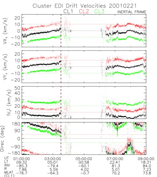
Fig. 8. Overview of drift velocities for 21 February in the same format as Fig. 4. Vertical dashed lines near 03:30 correspond to the first encounter with intense 1 keV electrons, as marked in Fig. 11.
distances of the order of the satellite separations, one expects that the satellite and plasma motion projected in this plane will provide a good basis for interpreting variations in elec-tron fluxes.
Similarly, in many cases, the drift velocity structures will also be ordered by structures perpendicular to the magnetic field. In addition to the satellite positions, each panel in Fig. 6 also shows the satellite velocity vector (solid line) and mag-netic field unit vector (dashed line). The velocity vector is scaled so that 1500 km on the distance axis corresponds to 5 km/s. The satellites are moving nearly perpendicular to the magnetic field, toward the equatorial plane (compare with Fig. 3).
In the B⊥ plane, spacecraft 1 is leading, followed by
spacecraft 3 and 2 at distances of about 800 and 1150 km, re-spectively, along the spacecraft velocity vector. In this plane,
the satellite velocity is primarily in the −X⊥direction,
cor-responding to the motion approximately in the meridianal plane toward the equator, with very little dawn-dusk com-ponent. Thus, the velocity is approximately perpendicular to
structures that are ordered by magnetic L-shells. With
satel-lite velocities in the B⊥plane of about 4.5 km/s, the
separa-tions given above correspond to time delays of approximately 3.0 and 4.3 min for spacecraft 3 and 2 with respect to space-craft 1.
Figure 7 shows the 1 keV ambient electron fluxes mea-sured by EDI as described in Sect. 2.3, using the standard colors for the three spacecraft. Each satellite detects a rela-tively sharp, × 100 increase in flux, separated by a few min-utes. Fiducial marks are plotted as vertical dashed lines at 13:12:30, 13:15:25, and 13:18:20 UT. The time differences between the spacecraft 1 encounter with the 1 keV electron boundary and those of spacecraft 3 and 2 are 2.9 and 5.8 min. Within the accuracy of placing the electron boundary cross-ings, the observed time delays are in good agreement with the times estimated above for crossing a static structure ori-ented along a magnetic field shell. The spacecraft 1–3 delay matches very closely the static boundary prediction (2.9 ver-sus 3.0 min). The longer spacecraft 1–2 delay differs more significantly from the prediction (5.8 versus 4.3 min). The
Fig. 9. Drift velocities during the 21 February southern hemisphere crossing from the polar cap into the high-latitude plasma sheet. Dashed markers plotted at the same times as those plotted in Fig. 8 and as the first set of markers in Fig. 11 indicate the satellites’ encounters with the first 1-keV electron structure.
discrepancy between the two pairs of delays may be due to the limited accuracy of identifying and timing the boundary crossings using a single electron energy, or it might imply true boundary motion during the interval between the en-counters by spacecraft 3 and 2. A precise interpretation of the boundary motion and the many detailed variations seen in Fig. 7 requires electron spectral information that is not avail-able in the standard EDI operations. From the 1 keV data, we conclude that the velocity of the boundary during the several minutes of the satellite crossings is lower than, or at most comparable to, the spacecraft velocities.
The times of the intense 1 keV electron encounters indi-cated in Fig. 7 are also marked in the drift velocity plots of Fig. 5. As seen on spacecraft 1, the 1 keV electron encounter slightly precedes the convection reversal that is seen in the
Y⊥(dawn-dusk) component and in the flow direction.
3.2 21 February 2001
We now turn to the Cluster perigee pass on 21 February 2001, one orbit before the 23 February perigee discussed above. The satellites’ orbits for this pass are very similar to that of 23 February, as shown in Fig. 3. Figure 8 shows an overview of EDI drift velocities for an 8-h period cen-tered on perigee, in the same format as Fig. 4. The flows are qualitatively similar to those on 23 February in several ways. As the satellites approach perigee through the south-ern polar cap (∼ 01:00–02:30 UT), the largest component of
the flow is anti-sunward. On both days, this X⊥ flow
de-creases while the duskward (−Y⊥) component of flow picks
up, although this change occurs over a longer interval on 21 February than on 23 February. As the satellites approach the auroral zone and plasma sheet, there is an interval of flow oscillations (beginning ∼ 03:10 UT), followed by a sudden
transition to highly variable flows and a reversal in the V Y⊥
Fig. 10. Spacecraft 1, 2, and 3 relative positions, with velocity and magnetic field, at the time of the first encounter with intense 1 keV electron counts (first markers in Fig. 11). Same format as Fig. 6.
Fig. 11. 1 keV ambient electron counts during the 21 February southern hemi-sphere crossing from the polar cap into the auroral zone/plasma sheet, whith the same format as Fig. 7. Counts for spacecraft 1 and 3 are offset by fac-tors of 1600 and 40, respectively. The first region of high counts, from approx-imately 03:30–03:45 UT, is a crossing of a spatial structure, as seen by the fact that the three spacecraft enter and exit the feature in the same sequence. Hor-izontal bands near the bottom of each plot represent discrete count levels of 2, 3, 4, etc. Count levels of 0 and 1 have been clipped.
with 23 February. A higher time resolution view of the south-ern hemisphere crossing from the polar cap into the plasma sheet is presented in Figs. 9 to 11, which show the flow ve-locities, relative satellite positions, and 1-keV electrons in the same formats, and with the same time scales, as the cor-responding figures for 23 February. As before, spacecraft 1 is the lead spacecraft, followed in turn by spacecraft 3 and 2. Figure 11 shows a more complicated and interesting structure at the electron boundary than was seen in the prior case. In particular, there are two distinct encounters with large 1-keV
electron features. The three sets of dashed vertical lines indi-cate the entry and exit for the first feature, and the entry into the second. In the first feature, at about 03:30–03:45 UT, the satellite sequence across both the leading and trailing edges (first and second sets of vertical lines) is in the same order
as their separation along the velocity vector in the B⊥plane.
This clearly establishes that the satellites are passing through an isolated feature, as opposed to having the boundary move across them and then back again (in which case, the order of exit would be opposite to the order of entry).
Superim-posed on and between the two large electron features are many smaller features that are probably the result of both satellite motion and time variations.
The convection velocities in Fig. 9 show a pronounced change at the time of the encounter with the first elec-tron structure in Fig. 11 (marked at 3:30:30, 3:31:45, and 3:32:30 UT in both figures). As in the previous case, the velocities change from relatively smooth to highly variable, and they remain so throughout the rest of the interval, includ-ing the period between the isolated electron structure and the boundary that is crossed between 4:05:00 and 4:07:30 UT.
As in the previous case, the dawn-dusk velocity compo-nent in Fig. 9 reverses its sign in the vicinity of the plasma sheet boundary. However, in this instance, the reversal oc-curs over a longer interval, apparently occurring in the region between the isolated structure and the subsequent boundary crossing.
4 Summary
We have presented initial multi-spacecraft EDI measure-ments during two perigee passes from the polar cap into the high-latitude plasma sheet boundary region at midnight. The EDI technique provides accurate measurements of the full E × B drift velocity, independent of the orientation of the magnetic and electric fields. Despite the complexities of EDI’s onboard beam-acquisition and tracking, the measure-ment is based upon simple geometry, yielding a well under-stood and reliable result. Throughout the two 8-h passes pre-sented here, there is close agreement in the measurements by the three spacecraft on coarse time scales. As expected, there are strong differences between the satellites on time scales comparable to their orbital separation during their encoun-ters with the plasma sheet boundary.
As the satellites approach the plasma sheet from the south-ern polar cap, the rather steady, primarily anti-sunward, flow decreases and becomes oscillatory. Near the plasma sheet boundary, the dawn-dusk component of the flow reverses. Within the plasma sheet, the flow velocities are much more variable, often showing significant differences between
con-secutive half-spin (2 s) measurements. However, on one
of the two days presented (23 February), the flow oscilla-tions are continuous across the boundary and well into the plasma sheet, indicating that the oscillation is rather
large-scale (∼ 10◦invariant latitude).
The multi-spacecraft observations of features in the elec-tron drift velocities, together with EDI’s measurement of 1 keV ambient electrons, are consistent with boundary struc-tures that are rather stable (moving at velocities less than the satellite velocities). Although the single-energy measure-ments presented cannot characterize the spectral and pitch angle structure of the electrons, they do provide a good proxy for plasma sheet entry as viewed from multiple satellites. In particular, on 23 February, the electron boundary is a sharp, single feature seen by all three satellites in sequence. In con-trast, on 21 February, there is a separate electron structure
poleward of the plasma sheet that is crossed by the satellites before entering the continous plasma sheet.
These initial observations illustrate that Cluster and EDI are well suited to investigations of the phenomena seen at the high-latitude plasma sheet boundary. We are beginning follow-on studies combining many different data sets to more fully characterize this rich region using the Cluster multi-point capabilities.
Acknowledgements. The authors thank the many people who have made the Electron Drift Instrument possible through years of de-velopment, testing, and operational support, in particular B. Austin, B. Briggs, J. Chan, M. Chutter, R. Frenzel, W. G¨obel, J. Googins, D. Hallmark, W. Isaac, G. King, S. Longworth, K. Lynch, R. Ma-heu, F. Melzner, J. Needell, U. Pagel, P. Parigger, D. Simpson, K. Strickler and C. Young. We acknowledge the excellent sup-port by the project team at ESTEC, in particular P. Escoubet and M. Fehringer, and the mission operations team at ESOC, in partic-ular S. Matussi and M. Schmidt. We are grateful to A. Balogh and the Cluster FGM team for their close collaboration in providing the onboard magnetic field data used by EDI and for use of the FGM data in EDI ground analyses; and to N. Cornilleau-Wehrlin and the STAFF team for providing the onboard STAFF data. We thank M. Goldstein, L. Christensen, and D. Machi for their key support of Cluster and EDI at NASA; and the payload team at Dornier, in par-ticular R. Nord. We acknowledge NASA SSCWeb for orbit plots. The authors remember fondly, and gratefully acknowledge, the pro-found contributions of N. Sckopke to EDI and Cluster, and the many pleasures brought by his presence and missed in his absence. This work was supported by NASA through grants NAS5-30744 and NAG5-9960, and by DLR through grants FKZ:50OC89043 and FKZ:50OC9705.
The Editor in Chief thanks M. Yamauchi an another referee for their help in evaluating this paper.
References
Baumjohann, W., Haerendel, G., and Melzner, F.: Magnetospheric convection observed between 06:00 and 21:00 LT: variations with Kp, J. Geophys. Res., 90, 393, 1985.
Carlson, C. W., McFadden, J. P., Ergun, R. E., Temerin, M., Peria, W., Mozer, F. S., Klumpar, D. M., Shelley, E. G., Peterson, W. K., Moebius, E., Elphic, R., Strangeway, R., Cattell, C. and Pfaff, R.: FAST observations in the downward auroral current region: Energetic upgoing electron beams, parallel potential drops, and ion heating, Geophys. Res. Lett., 25, 2017k, 1998.
Cattell, C. A., Kim, M., Lin, R. P., and Mozer, F. S.: Observations of large electric fields near the plasmasheet boundary by ISEE-1, Geophys. Res. Lett., 9, 539, 1982.
Eastman, T. E., Frank, L. A., Peterson, W. K., and Lennartsson, W.: The plasma sheet boundary layer, J. Geophys. Res., 89, 1553, 1984.
Melzner, F., Metzner, G., and Antrack, D.: The Geos electron beam experiment, S 329, Space Science Instrumentation, 4, 45, 1978. Mende, S. and Frey, H.: Image far ultraviolet instrument overview
plots, http://sprg.ssl.berkeley.edu/image/, 2001.
Paschmann, G., Melzner, F., Frenzel, R., Vaith, H., Parrigger, P., Pagel, U., Bauer, O. H., Haerendel, G., Baumjohann W., Sck-opke, N., Torbert, R. B., Briggs, B., Chan, J., Lynch, K., Morey, K., Quinn, J. M., Simpson, D., Young, C., McIlwain, C. E.,
Fil-lius, W., Kerr, S. S., Maheu, R., and Whipple, E. C.: The electron drift instrument for Cluster, Space Sci. Rev., 79, 233, 1997. Paschmann, G., McIlwain, C. E., Quinn, J. M., Torbert, R. B., and
Whipple, E. C.: The electron drift technique for measuring elec-tric and magnetic fields, Measurement Techniques in Space Plas-mas: Fields, Geophysical Monograph 103, AGU, 1998. Paschmann, G., Sckopke, N., Vaith, H., Quinn, J. M., Bauer, O. H.,
Baumjohann,W., Fillius, W., Haerendel, G., Kerr, S. S., Kletzing, C. A., Lynch, K., McIlwain, C. E., Torbert, R. B., and Whipple, E. C.: EDI electron gyro time measurements on Equator-S, Ann. Geophysicae, 17, 1513, 1999.
Paschmann, G., Quinn, J. M., Torbert, R. B., Vaith, H., McIlwain, C. E., Haerendel, G., Bauer,O. H., Bauer, T., Baumjohann, W., Filliius, W., Foerster, M., Frey, S., Kerr, S. S., Kletzing, C. A., Puhl-Quinn, P. and Whipple, E. C.: The electron drift instrument on Cluster: overview of first results, Ann. Geophysicae, (this is-sue) 2001.
Pederson, A., Cattell, C. A., Falthammer, C.-G., Knott, K., Lindqvist, P.-A., Manka, R. H., and Mozer, F. S.: Electric fields in the plasma sheet and plasma sheet boundary layer, J. Geophys. Res., 90, 1231, 1985.
Quinn, J. M., McIlwain, C. E., Haerendel, G., Melzner, F., Cauff-man, D., Measurement of vector electric fields using electron test particles, Trans., AGU, EOS, 60, 918, 1979.
Quinn, J. M., Paschmann, G., Sckopke, N., Jordanova, V. K., Vaith,
H., Bauer, O. H., Baumjohann, W., Fillius, W., Haerendel, G., Kerr, S. S., Kletzing, C. A., Lynch, K., McIlwain, C. E., Torbert, R. B., and Whipple, E. C.: EDI convection measurements at 5– 6 RE in the post-midnight region, Ann. Geophysicae, 17, 12, 1503–1512, 1999.
Sauvaud, J.-A., Popescu, D., Delcourt, D. C., Parks, G. K., Brit-tnacher, M., Sergeev,V., Kovrazhkin, R. A., Mukai, T., and Kokubun, S.: Sporadic plasma sheet ion injections into the high-altitude auroral bulge: Satellite observations, J. Geophys. Res., 104, 28 65, 1999.
Torbert, R. B. and Mozer, F. S.: Electrostatic shocks as the source of discrete auroral arcs, Geophys. Res. Lett., 5, 135, 1978. Vaith, H., Frenzel, R., Paschmann, G., and Melzner, F.: Electron
gyro time measurement technique for determining electric and magnetic fields, in: Measurement Techniques in Space Plasmas: Fields, (Eds) Pfaff, Borovsky, and Young, Geophysical Mono-graph, AGU, 103, 47, 1998.
Wygant, J. R., Keiling, A., Cattell, C. A., Johnson, M., Lysak, R. L., Temerin, M., Mozer, F. S., Kleting, C. A., Scudder, J. D., Pe-terson, W., Russell, C. T., Parks, G., Brittnacher, M., Germany, G., and Spann, J.: Polar spacecraft based comparisons of in-tense electric fields and Poynting flux near and within the plasma sheet-tail lobe boundary to UVI images: An energy source for the aurora, J. Geophys. Res., 18 675, 2000.