HAL Id: inria-00077051
https://hal.inria.fr/inria-00077051
Submitted on 29 May 2006
HAL is a multi-disciplinary open access
archive for the deposit and dissemination of sci-entific research documents, whether they are pub-lished or not. The documents may come from teaching and research institutions in France or abroad, or from public or private research centers.
L’archive ouverte pluridisciplinaire HAL, est destinée au dépôt et à la diffusion de documents scientifiques de niveau recherche, publiés ou non, émanant des établissements d’enseignement et de recherche français ou étrangers, des laboratoires publics ou privés.
Simulating Grid Schedulers with Deadlines and
Co-Allocation
Alexis Ballier, Eddy Caron, Dick Epema, Hashim Mohamed
To cite this version:
Alexis Ballier, Eddy Caron, Dick Epema, Hashim Mohamed. Simulating Grid Schedulers with Dead-lines and Co- Allocation. [Research Report] RR-5815, LIP RR-2006-01, INRIA, LIP. 2006. �inria-00077051�
ISSN 0249-6399
ISRN INRIA/RR--5815--FR+ENG
a p p o r t
d e r e c h e r c h e
Th `eme NUM
INSTITUT NATIONAL DE RECHERCHE EN INFORMATIQUE ET EN AUTOMATIQUE
Simulating Grid Schedulers with Deadlines and
Co-Allocation
Alexis Ballier — Eddy Caron — Dick Epema — Hashim Mohamed
N° 5815
Unit´e de recherche INRIA Rh ˆone-Alpes
655, avenue de l’Europe, 38334 Montbonnot Saint Ismier (France)
T´el´ephone : +33 4 76 61 52 00 — T ´el´ecopie +33 4 76 61 52 52
Simulating Grid Schedulers with Deadlines
and Co-Allocation
Alexis Ballier , Eddy Caron , Dick Epema , Hashim Mohamed
Th`eme NUM — Syst`emes num´eriquesProjet GRAAL
Rapport de recherche n 5815 — January 2006 —15pages
Abstract: One of the true challenges in resource management in grids is to
provide support for co-allocation, that is, the allocation of resources in multi-ples autonomous subsystems of a grid to single jobs. With reservation-based local schedulers, a grid scheduler can reserve processors with these schedulers to achieve simultaneous processor availability. However, with queuing-based local schedulers, it is much more difficult to guarantee this. In this paper we present mechanisms and policies for working around the lack of reservation mechanisms for jobs with deadlines that require co-allocation, and simulations of these mechanisms and policies.
Key-words: Grid, Scheduling, Simulation
This text is also available as a research report of the Laboratoire de l’Informatique du Parall´elisme http://www.ens-lyon.fr/LIP.
Simulation d’ordonnancement sur la Grille
avec deadlines et co-allocations
R´esum´e : Un des v´eritables d´efis pour la gestion des ressources dans les
envi-ronnements de type grilles est de fournir un support pour la co-allocation. La co-allocation est l’allocation des ressources dans des sous-syst`emes autonomes et diff´erents pour des tˆaches uniques. Aves des ordonnanceurs locaux `a base de r´eservation, un ordonnanceur de grille peut faire appel `a ces derniers pour r´eserver des processeurs afin d’utiliser efficacement les processeurs disponibles. Cependant, avec des ordonnanceurs locaux `a base de syst`eme batch, il est beau-coup plus difficile de garantir une utilisation efficace des processeurs. Dans cet article nous proposons des m´ecanismes et des politiques pour palier au manque de m´ecanismes de r´eservation avec une date limite que requiert la co-allocation. Nous avons r´ealis´e des simulations afin de valider ces m´ecanismes.
Simulating Grid Schedulers with Deadlines and Co-Allocation 3
1
Introduction
Over the past years, multi-cluster systems consisting of several to several tens of clusters containing a total of hundreds to thousands of cpus connected through a wide area network (wan) have become available. Examples of such
systems are the French Grid5000 system [3] and the Dutch Distributed ASCI
Supercomputer (das)[5]. One of the challenges in resource management in
such systems is to allow the jobs access to resources (processors, memory, etc.) in multiple locations simultaneously—so-called co-allocation. In order to use co-allocation, users submit jobs that consist of a set of components, each of which has to run on a single cluster. The principle of co-allocation is that the components of a single job have to start at the same time.
Co-allocation has already been studied with simulations and has been
proven as a viable option in previous studies [2, 6]. A well-known
imple-mentation of a co-allocation mechanism is duroc [4], which is also used in
the koala scheduler. koala is a processor and data co-allocator developed
for the das system [8, 7] that adds fault tolerance and scheduling policies to
duroc, and support for a range of job types.
One of the main difficulties of processor co-allocation is to have processors available in multiple clusters with autonomous schedulers at the same time. When such schedulers support (advance) reservations, a grid scheduler can try to reserve the same time slot with each of these schedulers. However, with queuing-based local schedulers such as SGE (now called SUN N1 Grid
Engine) [9], which is used in the DAS, this is of course not possible. Therefore,
we have designed and implemented in koala, which has been released in
the DAS for general use in september 2005 (www.st.ewi.tudelft.nl/koala),
mechanisms and policies for placing jobs (i.e., finding suitable executions sites for jobs) and for claiming processors before jobs are supposed to start in order to guarantee processor availability at their start time.
In this paper we present a simulation study of these mechanisms and poli-cies where we assume that jobs that require co-allocation have a (starting)
deadline attached to them. In Section 2, we describe the model we use for
the simulations, and in Section 3 we discuss and analyse the results of these
simulations. Finally, in Section 4 we conclude and introduce future work.
4 A. Ballier, E. Caron, D. Epema and H. Mohamed
2
The Model
In this section we describe the system and scheduling model to be used in our simulations. Our goal is to test different policies of grid schedulers with co-allocation and deadlines. With co-allocation, jobs may consist of separate components, each of which requires a certain number of processors in a single cluster. It is up to the grid scheduler to assign the components to the clusters. Deadlines allow a user to specify a precise job start time; when the job cannot be started at that time, its results will be useless or the system may just give up trying to schedule the job and leave it to the user to re-submit it.
One of the main problems of co-allocation is to ensure that all job com-ponents will be started at a specified time simultaneously. In queuing-based systems, there is no guarantee that the required processors will be free at a given time. On the other hand, busy processors may be freed on demand in order to accommodate a co-allocated (or global ) job that has reached its dead-line. Therefore, we assume that the possibility exists to kill jobs that do not require co-allocation (local jobs). In our model, the global jobs have deadlines at which they should start, otherwise they will be considered as failed.
As an alternative to this model (or rather, to the interpretation of dead-lines), one may consider jobs with components that have input files which first have to be moved to the locations where the components will run. When these locations have been fixed, we may estimate the file transfer times, and set the start time of a job as the time of fixing these locations plus the maximum transfer time. Then this start time can play the same role as a real deadline. The difference is that in our model, if the deadline is not met, the job fails, while in this alternative, the job may still be allowed to start, possibly at different locations.
2.1
System model
We assume a multicluster environment with C clusters, which for the sake of simplicity is considered to be homogeneous (e.g., every processor has the same power). We also assume in our simulations that all cluster are of identical size, which we denote by N the number of nodes. Each cluster has a local scheduler that applies the First Come First Served (FCFS) policy to single-component
Simulating Grid Schedulers with Deadlines and Co-Allocation 5
local jobs sent by the local users. The scheduler can kill those local jobs if needed. When they arrive, the new jobs requiring co-allocation are sent to a single global queue called the placement queue, and here the jobs wait to be assigned to some clusters.
In our model we only consider unordered jobs, which means that the ex-ecution sites of a job are not specified by the user, but that the scheduler must choose them. A Poisson arrival process is used for the jobs requiring co-allocation and for the single-component jobs for each cluster, with arrival
rates λg for global jobs and λl for the local ones in each cluster.
A job consists of a number of components that have to start simultaneously. The number of components in a multi-component job is generated from the uniform distribution on [2, C]. The number of components can be 1 only for local jobs which do not require co-allocation. The deadline for a job (or rather the time between its submission and its required start time) is also
chosen randomly with a uniform distribution on [Dmin, Dmax], for some Dmin
and Dmax. The number of processors needed by a component is taken from
the interval Is = [4, S], where S is the size of the smallest cluster. Each
component of a job will require the same number of processors. Two methods
are used to generate that size. The first is the uniform distribution on Is. The
second, which we have used in previous simulation work in order to have more
sizes that are power of two as well as more small sizes, is more realistic [2].
In this distribution, which we call the Realistic Synthetic Distribution, a job
component has a probability of qi/Q to be of size i if i is not a power of two,
and 3qi/Q to be of size i if i is a power of two. Here 0 < q < 1, and the value
of Q is chosen to make the sum of the probabilities equal to 1. The factor 3 is
made to increase the probability to have a size that is a power of 2 and qi to
increase the chance to have a small size.
Finally, the computation time of the job has an exponential distribution
with parameter µg for the global jobs and µl for the local jobs.
2.2
Scheduling Policies
In this section the so-called Repeated Placement Policy (RPP) will be de-scribed. Variations of this policy are used in the koala scheduler both for placing jobs and for claiming processors.
6 A. Ballier, E. Caron, D. Epema and H. Mohamed
Suppose a co-allocated job with deadline D is submitted at time S. The
RPP has a parameter Lp, 0 < Lp < 1, which is used in the following way. The
first placement try will be at time P T0, with:
P T0 = S + Lp·(D − S).
If placement does not succeed at P Tm, the next try will be at P Tm+1, defined
as:
P Tm+1 = P Tm+ Lp ·(D − P Tm).
As this policy can be applied forever, a limit on m has to be set, which will be
denoted Mp. If the job is not placed at P TM, it is considered as failed. When
a placement try is successful, the processors allocated to the job are claimed immediately. Note that with this policy, the global jobs are not necessarily scheduled in FCFS order.
In our simulations, the Worst Fit placement policy is used for job place-ment, which means that the components are placed on the clusters with the most idle processors. With this method, a sort of load balancing is performed. We assume that different components of the same job can be placed on the same cluster.
If the deadline of a newly submitted multi-component job is very far away in the future, it may be preferable to wait until a certain time before considering the job. The scheduler will simply ignore the job until T = D − I, where D is the deadline and I is the Ignore parameter of the scheduler. We will denote by Wait-X the policy with I = X. With set I to ∞, no job will ever be ignored. In our model, there are is a single global queue for the multi-components jobs, and a local queue for each cluster for single-component jobs. In order to give
global or local jobs priority, we define the following policies [1]:
GP: When a global job has reached its deadline and not sufficient processors
are idle, local jobs are killed.
LP: When we cannot claim sufficient numbers of processors for a global
multi-component job, that job fails.
Simulating Grid Schedulers with Deadlines and Co-Allocation 7
2.3
Performance metrics
In order to assess the performances of the different scheduling policies, we will use the following metrics:
The global job success rate: The percentage of co-allocated jobs that were
started successfully at their deadline.
The local job kill rate: The percentage of local jobs that have been killed.
The total load: The average percentage of busy processors over the entire
system.
The global load: The percentage of the total computing power that is used
for computing the global jobs. It represents the effective computing power that the scheduler has been able to get from the grid.
The processor wasted time: The percentage of the total computing power
that is wasted because of claiming processors before the actual deadlines of jobs.
3
Simulations
In this section we present our simulation results. We first discuss the param-eters of the simulation, then we simulate the pure Repeated Placing Policy, which does not ignore jobs, and finally discuss the Wait-X policies.
3.1
Setting the parameters
All our simulations are for a multicluster system consisting of 4 clusters of 32 processors each, and unless specified otherwise, the GP policy is used. The
number of processors needed by a local job (its size) is denoted Sl and is
generated on the interval [1; 32] with the Realistic Synthetic Distribution with
parameter q = 0.9. The expected value of Sl is E[Sl] = 6.95.
We set µl= 0.01 so that local jobs have an average runtime of 100 seconds.
Then the (requested) local load Ul in every cluster due to local jobs is equal
8 A. Ballier, E. Caron, D. Epema and H. Mohamed
to:
Ul =
λl·E[Sl]
µl·N .
We run simulations with a low local load of 30% and a high local load of 60%.
We denote by Sg the size of a component of a global job, which is taken
on the interval [4; 32] and which is also generated using the Realistic Synthetic
Distribution with parameter q = 0.9. The expected value of Sg is E[Sg] =
10.44. The number of components of a global job, Nc, is taken uniformally
on the interval [2; 4]. In our simulations we set µg = 0.005, so the global jobs
have an average runtime of 200 seconds. The (requested) global load, denoted
Ug, is given by:
Ug =
λg·E[Nc] · E[Sg]
µg·N · C .
It should be noted that we cannot compute the actual (local or global) load in the system. The reasons are that local jobs may be killed, there is processor wasted time because we claim processors early, and global jobs may fail because they don’t meet their deadlines. However, the useful load can be computed.
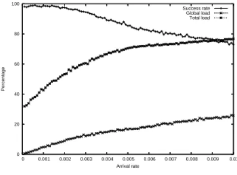
We run simulations with a low global load of 20% and a a high global load
of 40%. The results of a first general simulation, with Lp = 0.7, are shown in
Figure 1. 0 20 40 60 80 100 0 0.001 0.002 0.003 0.004 0.005 0.006 0.007 0.008 0.009 0.01 Percentage Arrival rate Success rate Global load Total load
Figure 1: Some metrics as a function of the arrival rate of global jobs with a low local load (30%).
Simulating Grid Schedulers with Deadlines and Co-Allocation 9
3.2
The Pure Repeated Placing Policy
In this section we study the influence of the parameters of the Repeated Placing Policy, which is nothing else than the Wait-∞ policy. The deadline is chosen
uniformally on the interval [1; 3599]. The parameter we vary is Lp.
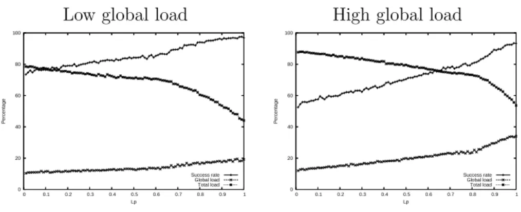
Low global load High global load
0 20 40 60 80 100 0 0.1 0.2 0.3 0.4 0.5 0.6 0.7 0.8 0.9 1 Percentage Lp Success rate Global load Total load 0 20 40 60 80 100 0 0.1 0.2 0.3 0.4 0.5 0.6 0.7 0.8 0.9 1 Percentage Lp Success rate Global load Total load
Figure 2: The influence of Lp with a low local load.
We first study the Wait-∞ policy with a low local load. We expected that
the success rate of global jobs will be higher for lower values of Lp, but this is
not the case, as shown in Figure2for a low local load. These results may seem
strange because RPP is designed to have a high success rate for global jobs. The processors for the global jobs are claimed earlier in order to ensure that their availability at the deadlines. In fact, the first jobs have indeed a greater success rate but the ones that come after them find fewer free processors, what causes them to fail. This analysis is clear when analysing the total load as a
function of Lp. It seems preferable to set Lp to 1 with any arrival rate of
the global jobs, at least for a low local load. However, the conclusion may be different with a high local load.
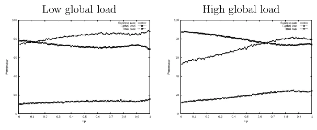
Therefore, we study the influence of Lp with a high local load (60%). The
results of those simulations shown in Figures 3 are very similar to the ones
with a low local load. The success rate decreases a little bit when Lp is close
to 1 when both the local and global loads are high, which is due to the fact that the total requested load is equal to 100%. This leads to the conclusion
10 A. Ballier, E. Caron, D. Epema and H. Mohamed
Low global load High global load
0 20 40 60 80 100 0 0.1 0.2 0.3 0.4 0.5 0.6 0.7 0.8 0.9 1 Percentage Lp Success rate Global load Total load 0 20 40 60 80 100 0 0.1 0.2 0.3 0.4 0.5 0.6 0.7 0.8 0.9 1 Percentage Lp Success rate Global load Total load
Figure 3: The influence of Lp with a high local load.
that the best way to meet the deadlines is simply to try to run the jobs at their starting deadlines with the hope that there will be enough free processors.
3.3
The Wait-X Policies
We have shown that the pure RPP (Wait-∞) is not efficient since a value of Lp
close to 1 is the best setting, which causes much processor time to be wasted.
However, as described in Section 2.2, it might be preferable to simply ignore
jobs until I seconds before their starting deadline. Since the scheduling policy may affect the results, we study both LP and GP policies. In this section we
fix Lp at 0.7.
According to the results shown in Figure 4, ignoring the jobs until 100
seconds or less before their starting deadline gives more or less the same results, while a pure RPP and ignoring until 1000 seconds before the deadline gives less good results. The Wait-0, Wait-10, and Wait-100 policies seem to be the most suitable choices for any arrival rate of the global jobs. We will prefer the Wait-10 policy to the two others because we want to have the possibility to place a job again in the case of failure, what we cannot do with the Wait-0 policy. We also do not want to have the overhead of applying the RPP over a too large interval of time.
The next parameter we investigated the influence of is the deadline (that is, the time between submission and required start time) of global jobs. Since
Simulating Grid Schedulers with Deadlines and Co-Allocation 11 0 20 40 60 80 100 0 0.002 0.004 0.006 0.008 0.01 Success rate Arrival rate Wait 0 Wait 10 Wait 100 Wait 1000 Wait Inf 0 20 40 60 80 100 0 0.002 0.004 0.006 0.008 0.01 Success rate Arrival rate Wait 0 Wait 10 Wait 100 Wait 1000 Wait Inf GP LP
Figure 4: Comparison of different ignoring policies with a low local load varying
the global arrival rate λg.
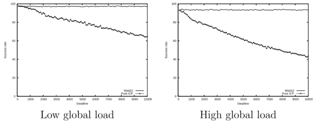
the Wait-10 policy was concluded to be the most suitable scheduling policy we compare it to the pure RPP. We compare the success rates of the global jobs
depending on their deadline. The results are in Figures 5and 6. As expected,
in both cases, the behavior of the Wait-10 scheduling policy is not affected by the value of the deadline, and the Wait-10 policy has better results than the pure RPP policy for any global load.
0 20 40 60 80 100 0 1000 2000 3000 4000 5000 6000 7000 8000 9000 10000 Success rate Deadline Wait10 Pure ICP 0 20 40 60 80 100 0 1000 2000 3000 4000 5000 6000 7000 8000 9000 10000 Success rate Deadline Wait10 Pure ICP
Low global load High global load
Figure 5: The influence of the deadline with a low local load.
We now study the influence of the load due to the single-component local jobs on both the RPP and the Wait-10 policies. The GP scheduling policy is
12 A. Ballier, E. Caron, D. Epema and H. Mohamed 0 20 40 60 80 100 0 1000 2000 3000 4000 5000 6000 7000 8000 9000 10000 Success rate Deadline Wait10 Pure ICP 0 20 40 60 80 100 0 1000 2000 3000 4000 5000 6000 7000 8000 9000 10000 Success rate Deadline Wait10 Pure ICP
Low global load High global load
Figure 6: The influence of the deadline with a high local load.
used because, with high local loads, the global jobs may not be able to run
with the LP policy. As shown in Figure7, the Wait-10 and pure RPP policies
have rather the same success rate while varying the local load.
0 20 40 60 80 100 0 0.01 0.02 0.03 0.04 0.05 Success rate
Local jobs arrival rate
Wait 10 Wait Inf
Figure 7: The influence of the local load on the Wait-10 and pure RPP policies with a low global load.
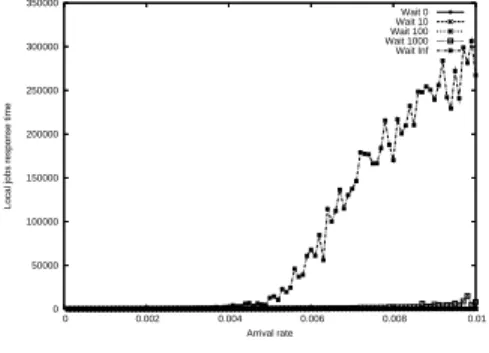
Finally, we trace the impact of the different scheduling policies on the local jobs. The policy will always be GP because a LP policy may not influence
the local jobs. As we can see in Figure 8, the pure RPP does not let the local
jobs run properly while the other policies are much nicer with them, with also better results for the global jobs as we have shown previously. The results
shown in Figure9are also in favor of the Wait-10 policy because when I is set
Simulating Grid Schedulers with Deadlines and Co-Allocation 13
to great values such as 1000 or ∞ there is a considerable amount of local jobs that are killed.
0 50000 100000 150000 200000 250000 300000 350000 0 0.002 0.004 0.006 0.008 0.01
Local jobs response time
Arrival rate Wait 0 Wait 10 Wait 100 Wait 1000 Wait Inf
Figure 8: The response time of local jobs as a function of the arrival rate of global jobs with different scheduling policies with a low local load.
0 20 40 60 80 100 0 0.002 0.004 0.006 0.008 0.01
Percentage of local jobs killed
Arrival rate Wait 0 Wait 10 Wait 100 Wait 1000 Wait Inf
Figure 9: The percentage of local jobs killed as a function of the global jobs arrival rate with different scheduling policies with a low local load.
4
Conclusions
In this paper we have presented a simulation study of grid schedulers with deadlines and co-allocation based on queuing-based local schedulers. We have shown that it is better to start considering jobs a short period of time before
14 A. Ballier, E. Caron, D. Epema and H. Mohamed
their deadline of global jobs. Considering the jobs too early may cause many jobs to fail; the first jobs, indeed, run fine but waste a lot of processor time, while the next ones do not have enough processors to run.
An extension to this work could be to consider the communication over-heads that happen on real grids. The Wait-10 policy which was concluded as the best policy may not be that good and the best value for I may depend on these overheads. We may also extend this work by considering the parameter I as a priority parameter. It may be interesting to consider the higher pri-oriy jobs earlier than the lower priority ones in order to ensure that the high priority jobs will run even if they waste a lot of processor time.
Acknowledgments
This work was carried out in the context of the Virtual Laboratory for e-Science
project (www.vl-e.nl), which is supported by a BSIK grant from the Dutch
Ministry of Education, Culture and Science (OC&W), and which is part of the ICT innovation program of the Dutch Ministry of Economic Affairs (EZ). In addition, this research work is carried out under the FP6 Network of Excellence CoreGRID funded by the European Commission (Contract IST-2002-004265).
References
[1] A.I.D. Bucur and D.H.J. Epema. Priorities among Multiple Queues for Processor Co-Allocation in Multicluster Systems. In Proc. of the 36th An-nual Simulation Symp., pages 15–27. IEEE Computer Society Press, 2003.
[2] A.I.D. Bucur and D.H.J. Epema. The Performance of Processor
Co-Allocation in Multicluster Systems. In Proc. of the 3rd IEEE/ACM Int’l Symp. on Cluster Computing and the GRID (CCGrid2003), pages 302–309. IEEE Computer Society Press, 2003.
[3] F. Cappello, E. Caron, M. Dayde, F. Desprez, E. Jeannot, Y. Jegou, S. Lanteri, J. Leduc, N. Melab, G. Mornet, R. Namyst, P. Primet, and
Simulating Grid Schedulers with Deadlines and Co-Allocation 15
O. Richard. Grid’5000: a large scale, reconfigurable, controlable and mon-itorable Grid platform. In Grid’2005 Workshop, Seattle, USA, November 13-14 2005. IEEE/ACM.
[4] K. Czajkowski, I. Foster, and C. Kesselman. Resource Co-Allocation in Computational Grids. In Proc. of the 8th IEEE Int’l Symp. on High Per-formance Distributed Computing (HPDC-8), pages 219–228, 1999.
[5] The Distributed ASCI Supercomputer (DAS). www.cs.vu.nl/das2.
[6] C. Ernemann, V. Hamscher, U. Schwiegelshohn, R. Yahyapour, and A. Streit. On Advantages of Grid Computing for Parallel Job Schedul-ing. In Proc. of the 2nd IEEE/ACM Int’l Symp. on Cluster Computing and the GRID (CCGrid2002), pages 39–46, 2002.
[7] Hashim H. Mohamed and Dick H. J. Epema. The design and implemen-tation of the KOALA co-allocating grid scheduler. In European Grid Con-ference, pages 640–650, 2005.
[8] H.H. Mohamed and D.H.J. Epema. Experiences with the koala Co-Allocating Scheduler in Multiclusters. In Proc. of the 5th IEEE/ACM Int’l Symp. on Cluster Computing and the GRID (CCGrid2005), 2005 (to
appear, see www.pds.ewi.tudelft.nl/~epema/publications.html).
[9] The Sun Grid Engine. http://gridengine.sunsource.net.
Unit´e de recherche INRIA Rh ˆone-Alpes
655, avenue de l’Europe - 38334 Montbonnot Saint-Ismier (France)
Unit´e de recherche INRIA Futurs : Parc Club Orsay Universit´e - ZAC des Vignes 4, rue Jacques Monod - 91893 ORSAY Cedex (France)
Unit´e de recherche INRIA Lorraine : LORIA, Technop ˆole de Nancy-Brabois - Campus scientifique 615, rue du Jardin Botanique - BP 101 - 54602 Villers-l`es-Nancy Cedex (France)
Unit´e de recherche INRIA Rennes : IRISA, Campus universitaire de Beaulieu - 35042 Rennes Cedex (France) Unit´e de recherche INRIA Rocquencourt : Domaine de Voluceau - Rocquencourt - BP 105 - 78153 Le Chesnay Cedex (France)
Unit´e de recherche INRIA Sophia Antipolis : 2004, route des Lucioles - BP 93 - 06902 Sophia Antipolis Cedex (France)
´ Editeur
INRIA - Domaine de Voluceau - Rocquencourt, BP 105 - 78153 Le Chesnay Cedex (France)
http://www.inria.fr