Analytical model for the prediction of pulsations in a cold-gas scale-model of a Solid Rocket Motor
18
0
0
Texte intégral
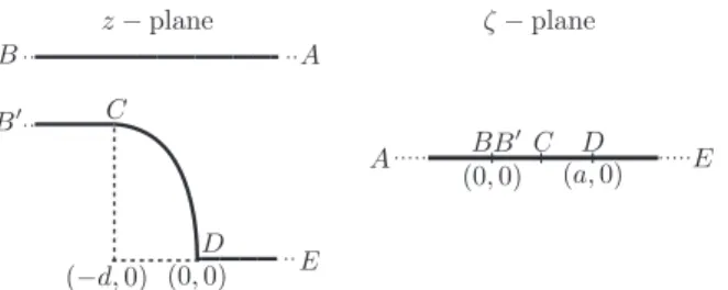
Figure

![Fig. 2 shows a sketch of the axial injection (1/30) scale model of the Ariane 5 booster used by Anthoine [17]](https://thumb-eu.123doks.com/thumbv2/123doknet/2973704.82841/4.816.242.576.804.986/shows-sketch-axial-injection-scale-ariane-booster-anthoine.webp)
![Fig. 5 shows the measurements from Anthoine [17] as a function of the Mach number for the second acoustic mode n = 2.](https://thumb-eu.123doks.com/thumbv2/123doknet/2973704.82841/12.816.250.571.749.1007/shows-measurements-anthoine-function-mach-number-second-acoustic.webp)
+4


Documents relatifs