Publisher’s version / Version de l'éditeur:
Proceedings of the 16th International Conference on Port and Ocean Engineering under Arctic Conditions POAC'01, pp. 505-515, 2001-08-12
READ THESE TERMS AND CONDITIONS CAREFULLY BEFORE USING THIS WEBSITE. https://nrc-publications.canada.ca/eng/copyright
Vous avez des questions? Nous pouvons vous aider. Pour communiquer directement avec un auteur, consultez la
première page de la revue dans laquelle son article a été publié afin de trouver ses coordonnées. Si vous n’arrivez pas à les repérer, communiquez avec nous à PublicationsArchive-ArchivesPublications@nrc-cnrc.gc.ca.
Questions? Contact the NRC Publications Archive team at
PublicationsArchive-ArchivesPublications@nrc-cnrc.gc.ca. If you wish to email the authors directly, please see the first page of the publication for their contact information.
NRC Publications Archive
Archives des publications du CNRC
This publication could be one of several versions: author’s original, accepted manuscript or the publisher’s version. / La version de cette publication peut être l’une des suivantes : la version prépublication de l’auteur, la version acceptée du manuscrit ou la version de l’éditeur.
Access and use of this website and the material on it are subject to the Terms and Conditions set forth at Numerical Simulation of the Broken Ice Zone Around the Molikpaq: Indications for Safe Evacuation
Barker, Anne; Timco, Garry; Sayed, Mohamed
https://publications-cnrc.canada.ca/fra/droits
L’accès à ce site Web et l’utilisation de son contenu sont assujettis aux conditions présentées dans le site LISEZ CES CONDITIONS ATTENTIVEMENT AVANT D’UTILISER CE SITE WEB.
NRC Publications Record / Notice d'Archives des publications de CNRC: https://nrc-publications.canada.ca/eng/view/object/?id=a85e9a77-34f2-433d-8447-929c4da47fc5 https://publications-cnrc.canada.ca/fra/voir/objet/?id=a85e9a77-34f2-433d-8447-929c4da47fc5
NUMERICAL SIMULATION OF THE BROKEN ICE ZONE AROUND THE MOLIKPAQ : IMPLICATIONS FOR SAFE EVACUATION
Anne Barker, Garry Timco and Mohamed Sayed Canadian Hydraulics Centre
National Research Council of Canada Ottawa, Ont. K1A 0R6, Canada
ABSTRACT
This paper presents an investigation of the zone of broken ice around the Molikpaq during interaction with moving ice. The width of this zone may have direct implications with respect to safe evacuation of personnel. A two-dimensional numerical model was used to study the size and behaviour of the broken ice zones with level ice interacting with both the long and short sides of the Molikpaq. Several scenarios of ice interaction with the Molikpaq were investigated. The results show the influence of ice thickness, ice velocity and approach angle of the ice upon sail height and rubble extent. A review of field observations obtained during operation of the Molikpaq shows that the model well predicts the zone of broken ice. The model can be used to evaluate emerge ncy evacuation systems for different structure shapes and ice conditions.
INTRODUCTION
Safe evacuation of personnel from offshore structures is of paramount importance in the event of a problem on the structure. There has been considerable work done on evacuation from offshore rigs and platforms in open water sea states (see e.g. http://www.nrc.ca/imd/eer/), but very little has been done for evacuation from structures in ice-covered waters, and many challenging problems remain. Evacuation in ice raises a number of different issues compared to evacuation onto water (Poplin et al. 1998a, 1998b; Polomoshnov, 1998). For an offshore caisson-type structure, the ice regime can be quite variable and safe approaches for evacuation must cover a wide range of ice conditions. When launching a lifeboat or other type of marine craft from an offshore structure, it is important to ensure that it does not get “caught” in the zone of ice broken by the structure during interaction with moving ice.
POAC ‘0 1
Ottawa, Canada
Proceedings of the 16 International Conference onth
Port and Ocean Engineering under Arctic Conditions POAC’01 August 12-17, 2001 Ottawa, Ontario, Canada
To investigate the size of these damage zones, an implicit Particle- in-Cell (iPIC) numerical model has been applied to a realistic situation of an offshore structure in a moving ice cover. In order to verify the qualitative and quantitative nature of the results, the model was applied to the offshore structure Molikpaq. This is a steel caisson structure that was used in the Beaufort Sea in the 1980s. Detailed information on the loads and ice conditions for this structure for each of the 4 years of its deployment in the Beaufort Sea is available (Timco, 1996). The iPIC numerical model was set-up using the Molikpaq geometry. A number of runs were carried out and compared to full-scale data. This paper presents a short description of the iPIC model, and presents the results of the numerical simulation. The results are compared to some representative results from the Molikpaq in the Beaufort Sea. The implications of the results are discussed in terms of emergency evacuation from structures in ice-covered waters.
OVERVIEW OF THE MODEL
The numerical approach is briefly outlined in this section with the intent to briefly convey the essential aspects of model formulation. A comprehensive treatment of the subject is outside the scope of this paper, and would be too lengthy to include here. Details of the present numerical formulation, however, were covered by Sayed and Carrieres (1999), who developed a version aimed at operational ice forecasting. The model was later adapted and validated for solving ice-structure interaction problems related to offshore ice-structures, with the Kulluk and bridge piers (Sayed et al. (2000), Barker et al. (2000a), and Barker et al. (2000b)).
The present model uses a continuum rheology that follows a Mohr-Coulomb plastic yield criterion. The governing equations consist of the continuum equations for the balance of linear momentum and the plastic yield criterion. Those equations are solved using a fixed grid. Advection and continuity, on the other hand, are handled in a Lagrangian manner. An implicit Particle-In-Cell (iPIC) approach is employed. In that approach, an assembly of discrete particles represents the ice cover. Each particle has a fixed volume, and is assigned an area and a thickness. At each time step the velocities are interpolated from the grid to the particles. Thus, particles can be individually advected. From the new positions, values of particle area and mass are mapped to the grid. The resulting ice mass and area for each grid cell are then used to update ice thickness and concentratio n. Solution of the governing equations can then be carried out using the fixed grid. An implicit finite difference method is used. That method is based on uncoupling the velocity components and a relaxation iterative scheme. Updated velocities and stressses on the fixed grid are obtained from the solution.
A depth-averaged implementation of the model is used in this paper, which averages the values of stresses and velocities over the thickness. Thickness variations, however, are accounted for. As stresses exceed a threshold, representing a ridging stress, each particle undergoes ridging; i.e. the thickness increases and area decreases, while conserving ice volume.
TEST RUNS AND COMPARISON TO FULL-SCALE DATA
The Molikpaq is a caisson structure that was used for exploration drilling for 4 seasons in the Canadian Beaufort Sea. It is a gravity-based structure that consists of an octagonal steel caisson annulus, with dredged sand placed in its central core. The caisson has outside dimensions of 111m at its base and 86m at its deck, and an overall height of 33.5m (including its 4.5m ice
deflector). At two of the drilling locations (the Tarsiut P-45 and Amauligak I-65 wellsites, drilled in 1984/85 and 1985/86 respectively), the Molikpaq was placed on a deep submerged berm with a set down depth of about 20m. With this deployment draft, the caisson’s walls were near vertical (8°) through the waterline. Because of this deployment configuration, there was no permanent accumulation of grounded ice rubble around the Molikpaq at either location. The caisson was directly exposed to moving pack ice throughout the winter. Since the pack ice was in near-continuous motion, a significant range of ice conditions moved past the Molikpaq over the course of these two winter seasons. The information from these sites was used in the present work for comparison with the output of the numerical model.
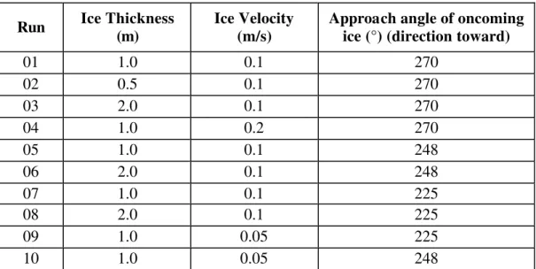
A total of ten runs were performed with the numerical model. The test runs were chosen such that ice properties and other parameters would represent conditions that are commonly encountered in the Beaufort Sea. The variables that could change between runs were the ice thickness (0.5 to 2m), ice velocity (0.05 to 0.2m/s) and the approach angle (225°, 248°, and 270°) of the oncoming ice (Table 1). The ice was initially “placed” upstream of the Molikpaq, with the initial ice concentration (or aerial coverage) set at 0.95. Each test was run for 5000s (2500 time steps). The grid node spacing in both the X- and Y-directions was 1m and the time step was set at 2s. The grid size was 500 nodes in the X-direction by 200 nodes in the Y-direction for runs 1 through 4 and 300 nodes by 400 nodes for runs 5 through 10. This change in grid size was necessary to accommodate the amount of ice required for the 248° and 225° approach angles. Node spacing and time step remained the same. The top edge of the grid (Y = 200m) is considered to be the north edge in later references.
Table 1 Test matrix Run Ice Thickness
(m)
Ice Velocity (m/s)
Approach angle of oncoming ice (°) (direction toward)
01 1.0 0.1 270 02 0.5 0.1 270 03 2.0 0.1 270 04 1.0 0.2 270 05 1.0 0.1 248 06 2.0 0.1 248 07 1.0 0.1 225 08 2.0 0.1 225 09 1.0 0.05 225 10 1.0 0.05 248
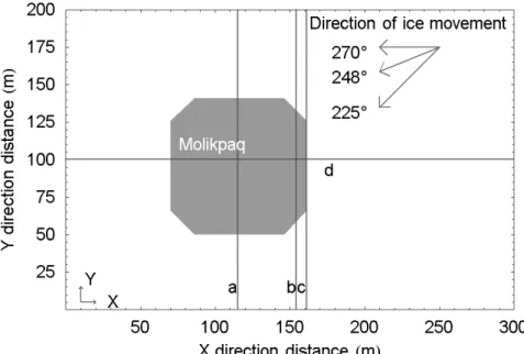
A schematic of the grid layout is shown in Figure 1. Lines “a”, “b”, “c” and “d” mark the locations of the cross-sections that are used to compare rubble heights over time. Line “c” is immediately in front of the Molikpaq and line “d” is perpendicular to the Molikpaq, parallel to the X-axis. Rubble extent is measured north and south from the edge of the structure where the cross-section is located, or in the case of line “c”, from the centreline of the structure. The rubble extent is taken as a minimum threshold value, calculated as a change in sail height greater than 0.2m from level ice, and only where the concentration of ice is greater than 0.5.
Figure 1 Schematic of the test area. Lines “a”, “b”, “c” and “d” mark the locations of the cross-sections that are used to compare rubble heights over time.
A plan view of the thickness contours after 5000s for Run_01 is shown in Figure 2. The contour levels are in 0.5m intervals, with minimum and maximum values of zero (white, representing the open water wake downstream of the Molikpaq), and 5m (black) respectively. A narrow wake forms at the west side (downstream) of the Molikpaq and the ice rubble surrounds the remaining three sides of the structure. It should be noted that the contours include both the sail region (which is observable from the structure) and the keel (which is under the ice sheet and not observable from the structure). This is an important point in comparing the results to full-scale conditions.
Information on level ice interaction with the Molikpaq was examined to quantitatively determine the regions of broken ice around the structure for different conditions. It was noted that the level ice interaction was characterised by 3 different failure modes – ice crushing, mixed mode failure and large-scale fracture. Representative values for the crushing and mixed mode failure were determined for an ice thickness of 1m. It was found that the width of the damage zone was different for the regions “updrift” of the structure and “alongside” the structure (see Figure 3). Moreover these widths were a function of the failure mode, with larger zones for mixed mode failures. In the “downdrift” region, there was generally open water, often mixed with broken ice pieces. Typical sizes and shapes for the 3 regions are shown in Figure 3.
Figure 2 Plan view of total thickness contours for Run_01 after 5000s. Contour levels are in 0.5m increments, with minimum and maximum values of zero (white), representing open water, and 5m (black), respectively. The dashed line indicates the extent of the sail of the ice rubble, with a sail height threshold of 0.2m.
Figure 3 Observations of ice damage zones around the Molikpaq for 1m thick level ice. Note that data are presented for 2 different failure modes.
Full-scale Observations
Ice Direction Open water
& brash ice
Ice crushing Mixed-mode failure 5 m 3 m UPDRIFT REGION DOWNDRIFT REGION ALONGSIDE REGION
Comparing the model results with the full-scale behaviour was not a trivial task. The full-scale data consist of visual observations taken from the top of the structure looking down towards the rubble field. As such, the observer is able to note the failure zone around the structure, but is unable to fully observe the whole rubble field and keel, which may be covered with snow or submerged. It would be difficult for an observer to note subtle differences in sail height, such as those less than 0.5m. The numerical model, on the other hand, provides different information. It cannot differentiate between the failure zone and the zone of accumulated ice. Therefore the output of the simulations depicts the entire rubble field.
In comparing Figure 2 to Figure 3, there is good qualitative correlation. The overall behaviour of the ice is the same. With the numerical model, the rubble extent of the sail extended about 25m in the updrift direction, which is larger than the observed values of 5m and 10m for ice crushing and mixed mode failures respectively. In the alongside direction, the extent of the rubble sail was calculated as 8m. The field observations were less than this, with values of 3m and 5m for crushing and mixed mode failures. In the downdrift section, the size and shape are the same in the model and the field; however, in the field, there are often broken ice pieces in the wake. Again, these differences are partly a result of the differences between what could be observed visually and partly due to the chosen threshold value.
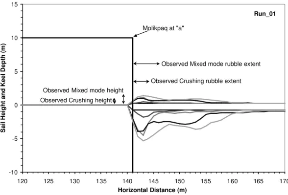
Figure 4 shows the evolution of sail and keel geometry at the north side of the Molikpaq, at cross-section “a” (see Figure 1 for location of the cross-section). Only this side of the test grid is shown in the figure, in order to compare the numerical results with representative values of the observed sail height and width of broken rubble, also presented on the figure, for both crushing and mixed mode failure. The cross-sections are plotted in terms of sail height and keel depth, instead of total thickness, to make it convenient for comparison with field observation. The figure shows sail heights and keel depths every 1000s. Since the ice rubble is neutrally buoyant, the ratio of sail height to keel depth is assumed to be 1:4, and is used to present the resulting cross sections. It can be seen that there is reasonable agreement between the observed sail heights and rubble extent and those from the numerical model. Note, however, the additional information on the extent of the keel portion of the ice is included in the results for the numerical model. This information is not observable in the full-scale situation.
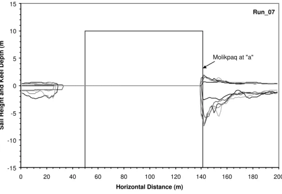
As an example of the effect of changing the angle of the oncoming ice, Figure 5 shows the ice thickness contours surrounding the Molikpaq for Run_07, and Figure 6 shows the sail and keel evolution. Both figures show that the open water wake shifts with the changing angle of the approaching ice. This results in open water along both the south and the west sides of the Molikpaq. When the ice approaches at 270°, as shown previously in Figure 2, only the west side of the Molikpaq had open water alongside.
Figure 7 shows a “rubble map” around the Molikpaq on 9 December 1984. This figure shows the situation with loading along a short side of the structure. Note the excellent agreement between the results from the numerical model and the full- scale situation.
-10 -5 0 5 10 15 120 125 130 135 140 145 150 155 160 165 170 Horizontal Distance (m)
Sail Height and Keel Depth (m)
Molikpaq at "a"
Observed Mixed mode rubble extent Observed Crushing rubble extent Observed Crushing height
Observed Mixed mode height
Run_01
Figure 4 Cross-section, for north side only, at “a” for Run_01 (x=115m) showing the time evolution of the ice rubble zone. Typical sizes for observed ice crushing and mixed mode failure regions for the Molikpaq are also indicated.
Figure 5 Plan view of total ice thickness contours for Run_07 after 5000s. Contour levels are in 0.5m increments, with minimum and maximum values of zero (white), representing open water, and 5m (black), respectively. The maximum sail height was 4.6m.
Run_07 -15 -10 -5 0 5 10 15 0 20 40 60 80 100 120 140 160 180 200 Horizontal Distance (m)
Sail Height and Keel Depth (m)
Molikpaq at "a"
Figure 6 Cross-section at “a” for Run_07 (x=115m)
Wake
(Choked with rubble) Wind Ice Cracks Cracks Advancing ice up to 1.2 m thick typically .7-.8 m Rubble extends 2 m from face Broken pieces floating free Crushed rubble 2 m high 5/10 Med FY ice 5/10 Thin FY ice Speed -- .05 m/s
Figure 7 Sketch from the Molikpaq logbooks showing the ice conditions around the Molikpaq on December 9, 1984. Note that the zone of broken ice is close to the structure and there is a large open area along the side and in the downdrift direction, in agreement the results from the numerical model.
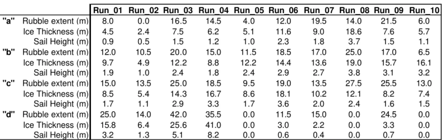
A comparison of results for the 10 test runs is shown in Table 2. For each run, and each cross-section, the table shows the maximum rubble extent from the face, the maximum ice thickness and the maximum sail height. These maximum values are taken after approximately 350m of ice have moved past the Molikpaq. As mentioned earlier, the maximum rubble extent is measured along a direction perpendicular to the north and south sides of the Molikpaq, and takes into
account a change in sail height greater than 0.2m and only where the concentration of ice is greater than 0.5; where the results are zero, one or both of these criteria were not met.
Table 2 Comparison of run results for each cross-section
Run_01 Run_02 Run_03 Run_04 Run_05 Run_06 Run_07 Run_08 Run_09 Run_10 "a" Rubble extent (m) 8.0 0.0 16.5 14.5 4.0 12.0 19.5 14.0 21.5 6.0
Ice Thickness (m) 4.5 2.4 7.5 6.2 5.1 11.6 9.0 18.6 7.6 5.7 Sail Height (m) 0.9 0.5 1.5 1.2 1.0 2.3 1.8 3.7 1.5 1.1 "b" Rubble extent (m) 12.0 10.5 20.0 15.0 11.5 18.5 17.0 25.0 17.0 6.5 Ice Thickness (m) 9.7 4.9 12.2 8.8 12.2 14.4 13.6 19.0 15.7 16.1 Sail Height (m) 1.9 1.0 2.4 1.8 2.4 2.9 2.7 3.8 3.1 3.2 "c" Rubble extent (m) 15.0 13.5 25.0 18.5 9.5 19.0 13.5 27.5 25.5 13.0 Ice Thickness (m) 8.5 5.4 14.3 16.7 8.6 18.1 10.2 12.1 8.2 7.4 Sail Height (m) 1.7 1.1 2.9 3.3 1.7 3.6 2.0 2.4 1.6 1.5 "d" Rubble extent (m) 25.0 14.0 42.0 35.5 0.0 11.5 15.0 0.0 24.5 0.0 Ice Thickness (m) 15.8 6.4 25.6 41.0 0.0 3.0 2.2 0.0 3.3 0.0 Sail Height (m) 3.2 1.3 5.1 8.2 0.0 0.6 0.4 0.0 0.7 0.0
Decreasing the angle of the oncoming ice had a varying effect on the rubble extent for both the 1.0m and 2.0m thick ice. Generally, the rubble extent increased with increasing ice thickness. The maximum rubble extent along a cross-section parallel to the Y-axis was 21.5m, observed during the case where the approaching ice was 1.0m thick, moving 225° towards the structure at 0.05m/s in Run_09. When examining the effects of increasing or decreasing the ice velocity, it was observed that the rubble extent results were inconclusive. Additional test runs are needed to provide more reliable results.
Along cross-section lines “a ” and “c”, when the ice velocity decreased, the sail height also decreased, and vice-versa. This was not the case along cross-section “b”, located at the corner of the Molikpaq, where the sail height increased with decreasing ice velocity. Increasing the ice thickness increased the sail height, and decreasing the ice thickness decreased the sail height, along all cross-sections. The sail height along the “a”, “b” and “c” cross-section lines generally increased with a decrease in the angle of the oncoming ice. The maximum sail height observed along the cross-sections parallel to the Y-axis was 3.8m, observed in Run_08, where the ice velocity was 0.1m/s, with 2.0m thick ice approaching at 225° towards the Molikpaq.
IMPLICATIONS FOR SAFE EVACUATION
Emergenc y evacuation from an offshore structure is complicated by the presence of moving ice. The present analysis of the field information and numerical model offer some guidance for a number of the key issues. For example, if the evacuation procedure involves launching a lifeboat from the structure, and since the ice can approach from any direction, the emergency evacuation system must have the flexibility to be quickly launched from any side. Additionally, unlike structures in ice-free conditions, lifeboats cannot be simply deposited a short distance from the structure. Evacuation procedures need to account for the generation of ice rubble around the structure. The failure zone of ice around the structure must be avoided, so that the lifeboats do not collide with the structure or get “caught” in the dynamic broken ice zone. However, lifeboats need only be launched a distance sufficient to clear this zone, as the keel of rubbled ice can provide additional buoyancy for a lifeboat.
Regarding the launch direction, as seen in Figures 2 and 3, launching in the updrift direction could be catastrophic since the ice would move the lifeboat back into the structure. Thus, launching in this direction must be avoided. If launching is done in the alongside direction, the launch distance must be larger than the width of the moving broken ice zone (the failure zone). Launching in the downdrift direction would put the lifeboat in ice-filled water and might be the best approach; however this is often the downwind direction, which could be problematic if there are toxic fumes from the structure. The information from Figures 5 to 7 show that there can be large open areas along two sides of the structure if the ice is moving in from an oblique direction. In terms of the distance the launch needs to be from the structure, using a threshold value of 0.2m to determine the extent of the rubble sail height, as mentioned previously, results in a conservative value for the rubble field. With a larger threshold value, the rubble extent would become smaller, or closer towards the structure, in keeping with the quantitative data from the full-scale observations. In practice, this would shorten the launch distance from the structure. The results from the numerical model provide additio nal details not observed from the field. For example, the extent of the accumulation of broken ice under the ice sheet can be seen from Figures 2, 4, 5 and 6. This broken ice would provide more buoyant support for loads put on top of the ice sheet and could add to the “effective” thickness of the ice for bearing capacity purposes. Note, however, that the majority of the ice accumulates in the updrift direction, with very little extent in the alongside direction. Therefore, this added buoyancy should not be considered in determining the bearing capacity of the ice.
The good agreement between the numerical model and the full-scale observations is encouraging. It illustrates that useful information can be obtained from the model. This type of analysis can be extended to structures with different shapes, and structures that are placed in different ice conditions. Also, the influence of grounded rubble could be considered with good confidence (see e.g. Barker et al. (2001) for a study on ice pile- up along shorelines and vertical structures). The present work has shown that a detailed numerical analysis of ice interacting with offshore structures can provide additional insight into the parameters that should be considered for emergency evacuation in ice-covered waters.
CONCLUSIONS
This paper examined the geometry of floating ice rubble formation around an offshore structure, the Molikpaq. Identifying the extent and height of ice rubble, as well as open water leads, due to ice movement against the structure is a necessary step for developing emergency evacuation systems. The present investigation employed a numerical model to simulate various scenarios of ice interaction with the Molikpaq. The model is based on an implicit Particle-In-Cell (iPIC) formulation and includes an efficient implicit numerical solution method. Rheology of the ice cover follows cohesionless Mohr-Coulomb yield criterion.
The numerical runs simulated several scenarios of ice interaction with the Molikpaq, which correspond to field observations. The numerical results were in good qualitative agreement with field observations. For example, the resulting extent and height of ice rubble, and the formation of open water were in accord with observations. A parametric study was carried out in order to examine the role of several parameters. The role of ice thickness, direction of ice movement, and velocity were examined. The numerical results indicated that the sail height generally increased
with decreasing approach angle and increasing thickness and velocity. The rubble extent increased with increasing ice thickness, but its relationship to ice velocity and approach angle was not as straightforward.
The present numerical simulations proved capable of predicting ice rubble accumulation and open water formation in the vicinity of offshore structures. The output could be used in evaluating emergency evacuation systems for different structure shapes and ice conditions.
ACKNOWLEDGEMENTS
The support of the Program on Energy Research and Deve lopment (PERD) is gratefully acknowledged.
REFERENCES
Barker, A., Timco, G. and Sayed, M. (2001). Three-Dimensional Numerical Simulation of Ice Pile-Up Evolution Along Shorelines. Proceedings 2001 Canadian Coastal Conference (in press), Québec City, Canada.
Barker, A., Timco, G. Sayed, M. and Wright, B.D. (2000a). Numerical Simulation of the “Kulluk” In Pack Ice Conditions. Proceedings 15th International IAHR Symposium on Ice, Vol. 1,
pp 165-171, Gdansk, Poland.
Barker, A., Sayed, M. and Timco, G.W. (2000b). Numerical Simulation of Floating Ice Forces on Bridge Piers. Proceedings 2000 Annual CSCE Conference, Vol. G, pp 243-249, London, Ont., Canada.
Polomoshnov, A. 1998. Scenario of Personnel Evacuation from Platform on Sakhalin Offshore in Winter Season. Proceedings International Conference on Marine Disasters: Forecast and
Reduction, pp 351-355, Beijing, China.
Poplin, J.P., Wang, A.T. and St. Lawrence, W. 1998a. Considerations for the Escape, Evacuation and Rescue from Offshore Platforms in Ice-Covered Waters. Proceedings International
Conference on Marine Disasters: Forecast and Reduction, pp 329-337, Beijing, China.
Poplin, J.P., Wang, A.T. and St. Lawrence, W. 1998b. Escape, Evacuation and Recovery Systems for Offshore Installations in Ice-Covered Waters. Proceedings International Conference on
Marine Disasters: Forecast and Reduction, pp 338-350, Beijing, China.
Sayed, M., and Carrieres, T. (1999). Overview of a New Operational Ice Forecasting Model,
ISOPE ’99. Vol. II, pp.622-627. Brest, France.
Sayed, M., Frederking, R. and Barker, A. (2000) Numerical Simulation of Pack Ice Forces on Structures: a Parametric Study. ISOPE ’00. Vol.1, pp.656-662. Seattle, U.S.A
Timco, G.W. 1996. NRC Centre of Ice/Structure Interaction: Archiving Beaufort Sea Data.