Application-aware deadlock-free oblivious routing

(1)

Application-Aware Deadlock-Free Oblivious Routing

by

Michel A. Kinsy

Submitted to the Department of Electrical Engineering and Computer Science

in partial fulfillment of the requirements for the degree of

Master of Science in Electrical Engineering and Computer Science

at the

MASSACHUSETTS INSTITUTE OF TECHNOLOGY

June 2009

@

Massachusetts Institute of Technology 2009. All rights reserved.

Author ... ...

...

Department of Electrical Engineering and CompL /Science

May 11, 2009

(n

Certified by ...

Srinivas Devadas

Professor of Electrical Engineering and Computer Science

Thesis Supervisor

...- ? n ,?

Accepted by ...

Terry P. Orlando

Chairman, Department Committee on Graduate Students

Department of Electrical Engineering and Computer Science

MASSACHUSETTS INSTiTUTE OF TECHNOLOGY

AUG 07RI ES2009

LIBRARIES

(2)

(3)

Application-Aware Deadlock-Free Oblivious Routing

by

Michel A. Kinsy

Submitted to the Department of Electrical Engineering and Computer Science on May 15, 2009, in partial fulfillment of the

requirements for the degree of

Master of Science in Electrical Engineering and Computer Science

Abstract

Systems that can be integrated on a single silicon die have become larger and increasingly complex, and wire designs as communication mechanisms for these systems on chip (SoC) have shown to be a limiting factor in their performance.

As an approach to remove the limitation of communication and to overcome wire de-lays, interconnection networks or Network-on-Chip (NoC) architectures have emerged. NoC architectures enable faster data communication between components and are more scalable. In designing NoC systems, there are three key issues; the topology, which directly de-pends on packaging technology and manufacturing costs, dictates the throughput and la-tency bounds of the network; the flit control protocol, which establishes how the network resources are allocated to packets exchanged between components; and finally, the rout-ing algorithm, which aims at optimizrout-ing network performance for some topology and flow control protocol by selecting appropriate paths for those packets.

Since the routing algorithm sits on top of the other layers of design, it is critical that routing is done in a matter that makes good usage of the resources of the network. Two main approaches to routing, oblivious and adaptive, have been followed in creating routing algorithms for these systems. Each approach has its pros and cons; oblivious routing, as opposite to adaptive routing, uses no network state information in determining routes at the cost of lower performance on certain applications, but has been widely used because of its simpler hardware requirements.

This thesis examines oblivious routing schemes for NoC architectures. It introduces various non-minimal, oblivious routing algorithms that globally allocate network bandwidth for a given application when estimated bandwidths for data transfers are provided, while ensuring deadlock freedom with no significant additional hardware.

The work presents and evaluates these oblivious routing algorithms which attempt to minimize the maximum channel load (MCL) across all network links in an effort to maximize application throughput. Simulation results from popular synthetic benchmarks and concrete applications, such as an H.264 decoder, show that it is possible to achieve better performance than traditional deterministic and oblivious routing schemes.

Thesis Supervisor: Srinivas Devadas

(4)

(5)

Acknowledgements

First, I would like to express my deep and sincere gratitude to Professor Srinivas Devadas for his extraordinary guidance, inexhaustible energy, and remarkable patience throughout this research. His support, encouragement, sound advice, and good teaching have been a true source of inspiration for me and I would have been lost without them.

I would like to thank Professor Edward Suh for his detailed and constructive comments, and for his important support throughout this work.

I am indebted to my many student colleagues for providing a stimulating and supportive environment in which to learn and conduct this research. I am especially grateful to Myong Hyon Cho for his participation in many aspects of this work, to Chih-chi Cheng for his help on the H.264 application, to Marten van Dijk for his valuable input and to Keun Sup Shim and Tina Wen for their help in generating simulation results.

I want to express my heartfelt gratitude to Myron King for his friendship in and out of the lab, to Charles O'Donnell for all his help on the formatting of the text, Mieszko Lis for his help with editing, and to Nirav Dave for his mentorship. I also thank Joel Emer, David Wentzlaff, Michael Pellauer, Bill Thies, and Vijay Ganesh for helpful comments on this research.

I am grateful to the Keller and Storace families for providing me a loving environment and to Dr. Sarma Vrudhula for his support and guidance.

Lastly, and most importantly, I wish to thank my parents and sister for their uncondi-tional and ever lasting love.

(6)

(7)

List of Figures

1-1 Resources and Switches Representation of 3 x 3 Mesh Network ... . 14

1-2 Node Representation of 3 x 3 Mesh Network . ... 14

1-3 Three Examples of Orthogonal Network Topology. . ... 15

1-4 Two Resource Interface Approaches. (a) External to the resource. (b) Inter-nal to the resource ... . .. ... 16

2-1 Example of Dimension Order Routing on 3 x 3 Mesh Network ... 21

2-2 Example of ROMM and Valiant on 3 x 3 Mesh Network . ... 21

2-3 Virtual Channels: (a) packet B is blocked behind packet A. (b) Virtual Chan-nels allow packet B to bypass blocked packet A. . ... 24

3-1 Channel Dependence Graph for the Mesh Network of Figure 1-2 ... 28

3-2 Two Turns Prohibited by the turn model. (a) North-Last turn. (b) West-First turn... ... ... . 30

3-3 Acyclic CDG Based of North-Last and West-First Prohibited Turns .... 30

3-4 (a) Acyclic CDG: 12 edges removed (b) Acyclic CDG: 12 edges removed . 31 3-5 Flow network from acyclic CDG of Figure 3-4 with source-destination pair A, L and example weights. . ... ... 33

3-6 (a) CDG for 2 x 2 sub-mesh FEAB with 2 virtual channels (b) Acyclic CDG using the turn model. (c) Ad hoc Acyclic CDG. . ... 36

3-7 Acyclic Virtual Networks for Multiple Virtual Channels . ... 38

4-1 Typical virtual-channel router architecture. The dark blue indicates that the modules and pipeline stages may be modified for our approach. ... . 39

4-2 The table-based routing architecture. (a) Source routing. (b) Node-table routing. ... ... ... 42

5-1 High-level Data flow description of H.264 decoder. . ... . . 47

5-2 Processor Performance Modeling Data Flow. ... 49

5-3 Wireless LAN Transmitter Data Flow. . ... .. 50

5-4 Transpose Node 52 Injection Rates when modeling burstiness ... . 50

6-1 Network Throughput and Average Latency graphs for Transpose Benchmark 54 6-2 Network Throughput and Average Latency graphs for Bit-Complement Bench-mark ... ... . 55

6-3 Network Throughput and Average Latency graphs for Shuffle Benchmark 56 6-4 Network Throughput and Average Latency graphs for H.264 Decoder Bench-mark ... . ... .... .. 57

(10)

6-5 Network Throughput and Average Latency graphs for Performance Modeling

Benchmark ... . . .. ... ... . 58

6-6 Network Throughput and Average Latency graphs for Transmitter Benchmark 59 6-7 Varying the number of VCs for transpose and H.264 Decoder. Results for

other examples show the same trend. . ... ... 60 6-8 The performance of various algorithms with 10% bandwidth variations . (a)

Transpose (b) H.264 . ... .. ... ... ... 60 6-9 The performance of various algorithms with 25% bandwidth variations . (a)

Transpose (b) H.264 ... . ... ... 61 6-10 The performance of various algorithms with 50% bandwidth variations . (a)

(11)

List of Tables

4.1 Router architecture designs for routing algorithms. . ... .. 40 5.1 H.264 profiling results for a standard input stream. . ... . 48 5.2 Estimates Data Rates for the IEEE 802.11a/g Wireless LAN Transmitter. . 48 6.1 Finding the routes with the minimum MCL (in MB/second) by exploring

different acyclic CDGs using BSORMILP. ... . . . . . . . ... 52 6.2 Finding the routes with the minimum MCL (in MB/second) by exploring

different acyclic CDGs using BSORDijkstra . ... 53 6.3 Comparison of Maximum Channel Load (MCL) in MB/second presented by

(12)

(13)

Chapter 1 Introduction

System-on-chip (SoC) designs typically contain a large number of heterogeneous digital components, such as processors, dedicated hardware engines, and memories, integrated onto a single chip. Traditionally, buses have been used in establishing communications between these different components, but because of the increasing complexity of these designs and the lack of scalability of wired connections between components, network-on-chip (NoC) architectures have been introduced as an effective data communication infrastructure [2, 44]. NoC architectures are characterized by an on-chip packet-switched micro-network of interconnects; they allow the digital components or resources in an SoC to communicate by sending packets to one another over that network. These architectures have resources or processing elements (PEs) attached to switches or routers, forming nodes that are linked together. Figure 1-1 illustrates such an architecture.

An NoC architecture is defined by its topology (the physical organization of nodes in the network), its flow control mechanism (which establishes the data formating, the switching protocol and the buffer allocation), and its routing algorithm (which determines the path selected by a packet to reach its destination under a given application). Figure 1-2 shows a two-dimensional 3 x 3 mesh network topology.

It has been shown that the overall performance of these systems is dominated not by the individual computation power of its resources, but by their communication limits in terms of bandwidth, speed and concurrency [23, 25, 30], in other words, the router architecture and the routing algorithm that are employed.

Because of the importance of the routing algorithm in affecting the overall performance, intensive research efforts have been put in developing algorithms that deliver high perfor-mance; unfortunately the vast majority of these algorithms have never been implemented because of the complexity of the router hardware that they require. Therefore, still relevant today is the challenge of designing routing algorithms which achieve good network load balancing, relatively short paths for packets, and simple router architecture.

(14)

Resource L Resource F Resource Hrc

Figure 1-1: Resources and Switches Representation of 3 x 3 Mesh Network

(15)

1.1 Topology of Networks-on-chip

The topology of an NoC is defined in terms of the theoretical shape formed by its nodes. Over the years, there have been a number of proposed topologies, but very few of them have ever been implemented in a real SoC. In today's Systems-on-chip, the most popular network topologies encountered are of the orthogonal shape; this means that the nodes are arranged in an orthogonal n-dimensional space, where each link between two nodes represents a displacement in a single dimension [15]. Figure 1-3 shows several of these topologies.

The popularity of these structures can be directly attributed to the simplicity of the router hardware needed to efficiently support them, because each node in the network can be assigned coordinates in the n-dimensional space and the router can use this underlying property of the topology to make forwarding decision with no overhead. To illustrate this work, the two-dimensional mesh topology has been adopted as shown in Figure 1-1, but the routing techniques presented are effectively topology independent.

1.2 Message Flow Control in Networks-on-chip

Flow control in NOCs architectures defines the unit of data in a given network, and deals with the mechanism for synchronizing the transmission and reception of these data units. Various techniques are used in allocating resources, namely channel bandwidth and buffers, needed by the data traversing the network.

With circuit switching, the network is first probed and physical channels are reserved from source to destination before packets are injected into the network. On the other hand in packet switching, when using store-and-forward or virtual cut-through, network resources are allocated on a per-hop basis. In the case of store-and-forward, a packet is forwarded to its next hop only when all its subparts are received, where cut-through starts the forwarding

(a) 3-ary 2-cube (b) three-dimensional mesh (c) hypercube

(16)

as soon as the packet's header is received. Another flow control mechanism frequently used is wormhole, where packets are further divided into flits, and resource allocation is done on a flit basis rather than on a packet basis. Intel's 80-core processor [561 uses a two-dimentional

mesh network that routes packets using wormhole routing.

Each of these approaches has its advantages and disadvantages; in this work we adopt the wormhole flow control technique, because of its efficient use of buffer space. The first flit of a packet is called the header flit. It holds the routing information about the packet, and sets up virtual channels for subsequent flits in the packet.

1.3 Network Resource Interface

Another important aspect of NoC design is the interface through which the network re-sources are integrated into the system. This aspect of the design deals with the conversion of data traffic, such as bus transactions, coming from the resources into packets or flits that can be routed inside the Network-on-chip, and the reconstruction of packets or flits into data traffic at the opposite side when exiting the NoC. Figure 1-4 (a) shows a typical approach used by designers when dealing with the processing element interface to the network.

Since the focus of this work is on routing techniques, the resource interface consideration has been put into the resource side of the overall system design [Figure 1-4 (b)].

Network

Interface

Logic

(a) External to resource (b) Internal to resource

Figure 1-4: Two Resource Interface Approaches. (a) External to the resource. (b) Internal to the resource.

(17)

1.4 Routing in Networks-on-chip

Routing algorithms for NoC architectures can be generally classified into oblivious and adaptive [3]. With oblivious routing, which includes deterministic routing algorithms as a subset, the path followed by a packet is statically determined. This allows each node in the network to make its routing decisions independently from the others. Due to this distributed aspect, oblivious routing, such as dimension order routing [1], enables simple and fast router designs, and is widely adopted in today's on-chip interconnection networks. But the drawback with oblivious algorithms is their poor performance when dealing with applications which contain certain communication patterns, e.g., bursty data transfers, because generally no application or network state information is used in computing routes. An adaptive routing algorithm, on the other hand, adjusts to the state of the network, using this state information, for example network congestion, in making routing decisions. With its dynamic load balancing, adaptive routing should theoretically outperform oblivious routing. However, adaptive routing schemes typically face the difficult challenge of balancing adaptiveness with router complexity. To achieve the best performance through adaptivity, a router ideally needs global knowledge of the current network status. However, due to router speed and complexity, dynamically obtaining a global and instantaneous view of the network is often impractical. As a result, adaptive routing in practice relies primarily on local knowledge, which limits its effectiveness.

These routing algorithms can be further classified as minimal and non-minimal. Minimal routing schemes only select paths that are the shortest possible routes between source and destination pairs. In Figure 1-2, for example, a packet traveling from node L to node B has three minimal path choices (L, H, E, B); (L, F, A, B) and (L, F, E, B). Although for applications for which latency is critical and should be minimized, minimal routing is desirable, it may exhibit poor load balancing over a range of applications.

Non-minimal routing sacrifices locality for better load balancing. Since it is less con-strained in its path selection, it generally leads to lower network congestion and overall better network throughput [32]. For a given flow, latency may increase.

1.5 Contributions

In this work, a bandwidth-sensitive oblivious routing (BSOR) scheme that statically deter-mines routes considering an application's communication characteristics is developed and evaluated. The main challenge with any oblivious routing is a fair and an effective trade-off between load balancing and communication latency minimization. Here the proposed oblivious routing scheme uses a function corresponding to minimizing the maximum chan-nel load (MCL) across all network links, while providing a mechanism for controlling the average path length. The core premise of this approach is to efficiently balance network

(18)

load while having shortest possible path lengths and keeping the router architecture simple and practical. To that end, the algorithm exploits knowledge of estimated bandwidths for all or a subset of data transfers in a given application, and focuses on optimizing satisfac-tion of bandwidth demand and latency of individual data transfers. This scheme is livelock and deadlock free and produces routes that can be minimal or non-minimal in an effort to globally optimize application throughput.

This scheme will be particularly suitable for long-running applications with predictable communication patterns. For example, the approach is suitable for co-processing platforms such as reconfigurable hardware, where processing elements and their interconnection net-work can be configured much like an FPGA to speed up a computationally-intensive task such as video compression, processor simulation, or rendering. In reconfigurable comput-ing, a computation is spatially partitioned into processing elements (PEs) and the network traffic pattern remains relatively static as each PE performs a fixed task. Evaluations on synthetic traffic with various patterns and applications such as H.264 decoding and pro-cessor performance modeling even when the network traffic varies at run-time due to data dependent behaviors show throughput improvements over traditional oblivious routing.

1.6 Organization

The rest of this thesis is structured as follows. Chapter 2 begins with a review of widely used oblivious routing algorithms followed by a short descriptive summary of previously proposed application-specific routing algorithms.

Chapter 3 formally presents our bandwidth-sensitive oblivious routing algorithm, and its synthesis flow for both small and large size problems to ensure scalability of the algorithm. Chapter 4 explores the router architecture needed to support the proposed bandwidth sensitive approach by taking a typical virtual-channel router architecture, and showing the modifications required.

Chapter 5 presents the illustrating applications followed by Chapter 6 where the exper-imental results are evaluated.

(19)

Chapter 2 Background and Related Work

Routing algorithms for on-chip networks have been a subject of research in both academia and industry for decades because they are aimed at solving a problem with many conflicting aspects [48], such as minimizing the router logic while efficiently balancing the network data traffic load. Oblivious routing algorithms generally lead to simpler hardware, and are very popular in systems being currently deployed, but for the most part they suffer from lack of good load balancing. Application-specific routing algorithms in their attempt to solve this problem, have been done largely using adaptive routing frameworks which essentially leads to larger and more complex hardware. For a recent survey on network-on-chip in general see [49].

2.1 Oblivious Routing Algorithms

Oblivious routing algorithms are broadly classified into two main categories, deterministic and non-deterministic routing schemes. With deterministic routing, the same route is always taken for any given pair of nodes. Non-deterministic routing uses randomness to archive better path diversity.

2.1.1 Deterministic Routing Algorithms

The two widely used deterministic routing algorithms are dimension order routing and

destination-tag routing.

Dimension order routing (DOR) algorithms [7] are vastly popular and have many de-sirable properties, for example they generate deadlock-free routes in mesh or hypercube topologies [1, 45]. Either using XY-ordered or YX-ordered routing, each packet is routed along one dimension in its first phase followed by the other dimension. Figure 2-1 shows examples of these routing schemes. The strength of these algorithms is their high com-patibility with orthogonal topologies and the low level of hardware complexity needed to

(20)

support their implementations. DOR algorithms, even with their lack of path diversity and network load balancing, which lead to poor network bandwidth utilization and low perfor-mance throughput, are frequently used by designers to avoid additional hardware overhead. They are in fact used in many commercial and research products: Intel Paragon, Cray T3D, MIT J-machine and Stanford DASH all use some version of DOR as their routing algorithm

[15, 27].

Destination-tag routing was initially designed by Lawrie [6] to allow concurrent, collision-free access to various data banks of a primary memory system by an array of processors. It later became very useful for routing packets in butterfly networks, where the digits representing the destination address are used by hops to determine the proper output port to which to forward a given packet [27]. Many research prototype and commercial computers use this routing scheme; BBN Butterfly, IBM RP3, NYU Ultracomputer, and NEC Cenju-3 all use some version of destination-tag routing.

2.1.2 Non-Deterministic Routing Algorithms

Valiant [8] and ROMM [17] have generally served as the representatives of this class of routing algorithms.

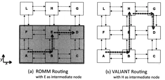
Valiant et al propose two different versions of an algorithm which routes a packet from its source to its destination in multi-phase fashion [8]. The routing algorithm selects at random an intermediate node and in the first stage of the routing the packet is sent from the source to the intermediate node, then in the second stage from the intermediate node to its official destination. Figure 2-2 shows an example of this Valiant algorithm. Although an arbitrary routing algorithm can be used for each of the phases, generally a simple DOR algorithm is used. It is shown to provide a good network load balance but can also lead to considerably longer path lengths. Towles et al further refine the Valiant algorithm to eliminate loops in the routes, and reduce the average path length by 20% [33].

ROMM routing which stands for randomized, oblivious, multiphase, minimal routing, was design by Nesson and Johnsson as an alternative to Valiant. In an effort to retain locality in routing of packets in the network, the intermediate node random selection is confined to a minimal quadrant [17] as illustrated in Figure 2-2. This approach essentially translates into randomly selecting between the various minimal paths from the source to the destination.

In Orthogonal one-turn routing (O1TURN routing) [46], which can be described as a restricted version of ROMM routing where the intermediate node is one of four corners of the minimum rectangle, Seo et al show that simply balancing traffic between XY and YX routing can guarantee provable worst-case throughput while reserving the same degree of router complexity.

(21)

2.2 Application-Specific Routing Algorithms

In this section we briefly survey several proposed routing algorithms that use targeted appli-cation information to provide higher performance in NoC architectures; see [49] for a recent more detailed survey. Application-specific routing schemes have generally approached the load balancing problem in two ways; either by designing algorithms to optimize performance for some subset of applications with little or no change to the targeted router architecture or by proposing algorithms that require their own router architecture and/or topology.

Palesi et al [52, 59] provide a framework and algorithms for application-specific bandwidth-aware deadlock-free adaptive routing. Given the communication graph of an application, cycles are eliminated from the channel dependency graph (CDG) to minimize the impact

L H C L H G

F E D F E D

(a) XY-ordered Routing (b) YX-ordered Routing

Figure 2-1: Example of Dimension Order Routing on 3 x 3 Mesh Network

L H G

yt

(a) ROMM Routing

with E as intermediate node

(b) VALIANT Routing

with H as intermediate node

(22)

on the average degree of adaptiveness. Bandwidth requirements are taken into account to spread traffic uniformly through the network. Their Application Specific Routing

Algo-rithms (APSRAs) rely on the fact that the network router architecture is adaptive, and the

designer's willingness to further increase the router area of the system.

Hansson et al [43) propose a unified approach to mapping and routing to minimize the network required to satisfy the constraints of the application. They show that overhead for this unified approach is only 20% higher than that of path selection alone in terms of run-time. The comparison is done against another approach [42] which generates network topology and mapping based on application specifications.

Many works on mapping of applications onto NoC architectures have also considered the routing problem during the NoC design phase (e.g., [31], [41], [50]).

Cho et al describe bandwidth-aware routing for diastolic arrays [57] and avoid deadlock by assuming that each flow has its own private virtual channel. Although this assumption simplifies deadlock avoidance in the routing algorithm, it may not be practical in cases where the number of flows traversing a router exceeds the number of allowed virtual channels.

Murali et al [40] present a tool for automatically selecting the best topology for a given application and producing a mapping of cores onto that topology. Although their SUNMAP algorithm supports different routing functions and takes into account bandwidth and area constraints, the direct impact of the routing functions on the overall performance of the network was not explored.

Srinivasan et al [47] using application specifications propose a slicing tree based floor-planner for the topology design. This technique does not insure deadlock-free routes which is crucial in packet-based NoC architectures.

Designing a network topology based of a application, though it has its advantages, presents the system designer with the choice of supporting only a small subset of applications that are part of the application class for which the topology is designed; or having different topologies for different classes of applications. The manufacturing cost of both of these

choices, have made application-specific topologies highly unattractive in the larger domain of NoC architectures.

2.3 Buffer Space and Bandwidth Allocation

Several approaches to allocate buffer space and bandwidth in on-chip networks have been proposed. Most routing strategies group packets that need to be in-order at the receiver into a flow, and packets of a flow follow a single path (e.g., [12], [21]). Flows are then routed based on the routing algorithm adopted by the designer and this routing algorithm dictates the bandwidth and the buffer space allocation in the network.

(23)

2.3.1 Buffer Space Allocation

Buffers in NoC architectures generally occupy most of the physical area allocated to the router [29, 36]. So designers are forced to keep the number of buffers fairly small and make judicious use of that limited amount of buffering space. Dally's virtual channels [9] allocate buffer space for virtual channels in a way that is decoupled from bandwidth allocation. In his approach, each physical channel is associated with several small buffers, virtual channels, which compete with each other for the physical channel. This decoupling allows active flows to use network bandwidth more efficiently.

iWarp [64], is a system architecture for high-speed signal, image, and scientific comput-ing, which implements virtual channels across single links. Its processing elements use these logical (virtual) channels to guarantee bandwidth to virtual circuits.

Hu and Marculescu, in their application-specific buffer allocation scheme, perform buffer allocation based on arrival rates [36]. More precisely, given the communication character-istics of an application and buffer space available in the network, their algorithm auto-matically assigns the buffer depth for each input channel, in different routers across the

network.

Many other designs of virtual channel routers have been proposed. Nicopoulos et al have designed a dynamic virtual channel regulator called ViChaR, which dynamically allocates buffering resources depending on the network state [51]. Their approach aims at maximizing throughput by allocating virtual channels on demand. Mullin et al propose in [39] a router design for which the arbitration logic is removed from the the critical path in oder to im-prove the cycle-time. Bjerregaard and Sparso present two different non-blocking schemes in implementing virtual channels with minimal hardware overhead [35]. Kavaldjiev et al have proposed a 5-port virtual channel router architecture with simplified dynamic arbitration which allows fair and deterministic arbitration [38]. They claim that such an architecture reduces the area allocated to routing by 23% over an ASIC implementation and produces a speed improvement of 1.4X when compared to a conventional router.

Recently, express virtual channels have been proposed which skip routers along multiple-hop static paths to enhance performance in a dynamic routing scheme [28]. Support for multicast channels has also been proposed [58].

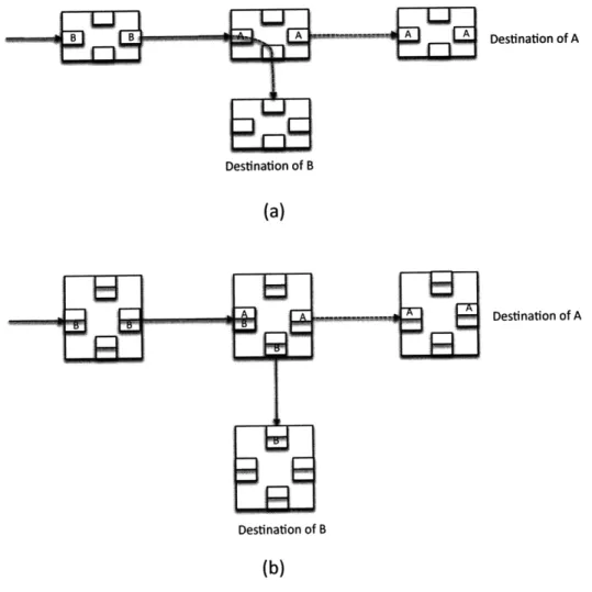
The partition of the router buffer space into virtual channels, either in a linked-list or disjoint forms, like those shown above, helps mitigate the head-of-line blocking issue that arises in NoC routing. Figure 2-3 shows how active flows can bypass blocked flows to use network bandwidth that would otherwise remain idle.

Our virtual channel router design is fairly standard and is described in Chapter 4. Our algorithms for static allocation assign flows to channels/lanes on a per-link basis, rather than assigning packets to a particular lane through the entire route.

(24)

2.3.2 Bandwidth Allocation

Bandwidth allocation to data flows in a given application is at the heart of the routing problem. An effective routing algorithm allocates bandwidth to flows in a way that balances the traffic loads across channels and provides application with a throughput close to the network ideal throughput. One approach is to formulate the bandwidth allocation problem as a linear programming problem.

Towles et al [34] give a multicommodity flow linear programming formulation for router algorithm design. When the linear program is optimized, deterministic algorithms that are worst case or average case optimal come out as solutions.

Racke uses concurrent multicommodity flow (CMCF) formulation to present his frame-work for solving on-line problems that aim to minimize the congestion in different netframe-works [261. Routing paths are selected according to the solution of the CMCF problem. His

obliv-- Destination of A Destination of B (a) Destination of A Destination of B

(b)

Figure 2-3: Virtual Channels: (a) packet B is blocked behind packet A. (b) Virtual Channels allow packet B to bypass blocked packet A.

(25)

ious path selection algorithm has a polylogarithmic competitive ratio in general networks. Our goal is to find routes with maximal throughput for a specific application.

2.4 Adaptive Routing Algorithms

Classic adaptive routing schemes include the turn model routing methods [11] and odd even routing [22]. In [37] a hybrid scheme that switches between deterministic and adaptive modes depending on the application is presented, where local FIFO information is used to adapt routes. Duato (e.g., [4, 14]) gives necessary and sufficient conditions for adaptive routing in wormhole networks. Our algorithm is not adaptive; however, as described in chapter 3, we use the turn model to derive an acyclic channel dependence graph that drives our oblivious routing scheme. Our scheme can use cycle-breaking strategies other than using the turn model in the derivation of acyclic dependence graphs.

To summarize our framework is significantly different from previous work in its use of application specifications to efficiently balance network load while retaining an oblivious nature and an applicability to standard router architectures.

(26)

(27)

Chapter 3 Oblivious Routing with Bandwidth

Sensitivity

The proposed Bandwidth-Sensitive Oblivious Routing (BSOR) algorithm exploits knowledge of estimated bandwidths for all or a subset of data transfers between modules for a given ap-plication in producing routes that globally optimize the apap-plication throughput. Although a two-dimensional mesh network topology is adopted in illustrating BSOR in this work, the algorithm is independent of both network topology and number of virtual channels per link. To present BSOR, the routing problem is formulated as a multicommodity-flow problem and the following standard definitions of flow networks and channel dependence graphs are used.

3.1 Definitions

Definition 1. Given a flow graph G(V, E), where an edge (u, v) E E has capacity c(u, v). The capacities c(u, v) are the available bandwidths on the edge. There is a set of k data transfers or flows K = {K 1, K2,..., Kk}. Ki - (si, ti, di), where si and ti are the source

and sink, respectively, for connection i, and di is the demand. We assume si 0 ti. We may have multiple flows with the same source and destination. The flow variable i along edge (u, v) is fi(u, v). A route is a path pi from si to ti for a flow i. Edges along this path will have fi(u, v) > 0, other edges will have fi(u, v) = 0.

If fi (u, v) > 0, then route pi will use both bandwidth and buffer space on the edge (u, v). The value of fi(u, v) indicates the amount of bandwidth allocated to flow i on the edge. In the case of single path flows fi(u, v) is equal to di. The buffer resource may be a packet buffer in the case of packet-buffer flow control, or a virtual channel in the case of flit-buffer flow control. We will assume flit-buffer flow control in this work, although our framework can be applied to other flow control schemes as well.

(28)

net-work G as follows. Each vertex in V' is an edge in G. There is an edge from vl E V' to

v2 E V' if a packet can flow from the edge in G associated with vl into the edge associated

with v2, without traversing any other edges. That is, the edges are consecutive in G. We are disallowing 180-degree turns in routing and will later remove these edges.

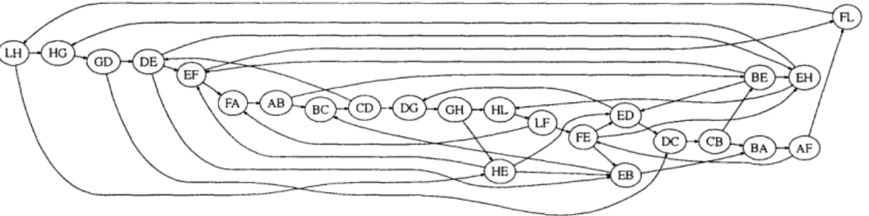
Figure 3-1 shows the CDG associated with the 3 x 3 mesh network in Figure 1-2 BC and CB are edges in opposite directions from B to C and C to B, respectively. They

correspond to separate vertices in the CDG and are not connected when 180-degree turns are not allowed. Note that the CDG has cycles, for example, there are edges connecting DG to DH, DH to HE, HE to ED and ED to DG.

Definition 3. The maximum channel load (MCL) U in a network is defined as

k

U = max

f

(uv) (3.1)

(u,v)EE i=1

It denotes the channel with the highest load which is the bottleneck channel in the entire network and determines the saturation throughput of the system.

Definition 4. For a given set of k data transfers or flows K = {K1, K2,..., Kk}, let

SF be the selector function that chooses the path pi taken by packets of flow i from si to ti through the network.

We define load balancing to be the degree to which resources in term of bandwidth and buffer space are uniformly utilized across the different links of the network; and latency as the required time or number of hops to router a packet from its source to the destination.

3.2 BSOR Framework

The BSOR algorithm uses the estimated bandwidths of an application and the targeted net-work topology and resource information to make advance plans to provide load balancing

(29)

during run-time of the application. It follows the framework outlined below; and many dif-ferent bandwidth-sentive algorithms can be constructed based on the framework depending on the selector function SF. For this work, we detail two instantiations of the framework, one using Mixed Integer Linear Programming (MILP) for small and medium size problems and the other using Dijkstra's weighted shortest path algorithm, for large size problems.

FRAMEWORK(Data Transfers K)

1. Create an acyclic channel dependence graph (CDG) by deleting edges from D; call it DA.

2. Transform DA into a flow network GA.

3. Choose routes pi for each flow i in GA, taking into account bandwidth availability using an SF.

4. If desired, go to Step 1 to create a different acyclic CDG and repeat. 5. Select the best set of routes found.

Offline Bandwidth-Sensitive Oblivious Routing Framework

This framework assumes that the underlying network has been made deadlock free. Deadlock in NoCs occurs when two or more flows are each waiting for the other to release link or buffer space in effort to finish routing a packet to its destination. Although there are techniques for recovering from a deadlock in these systems, performance can suffer a great deal and hardware complexity increases drastically. The usage of the acyclic chan-nel dependence graph in step one ensures the deadlock freedom property of the routing

algorithm.

Lemma 1. A routing algorithm R is deadlock-free if and only if the set of routes it

produces forms an acyclic channel dependence graph (CDGA) [1].

Dally and Aoki in [10] give the formal proof for Lemma 1.

3.3 Creating Acyclic Channel Dependence Graphs

According to Lemma 1, if packets follow routes that conform to an acyclic channel depen-dence graph, then deadlock will not occur. This is also a necessary condition provided false resource dependences do not exist [20].

Therefore, routing of packets is systematically restricted by breaking all the cycles in the CDG D associated with the network. There are many ways to remove these cycles; the

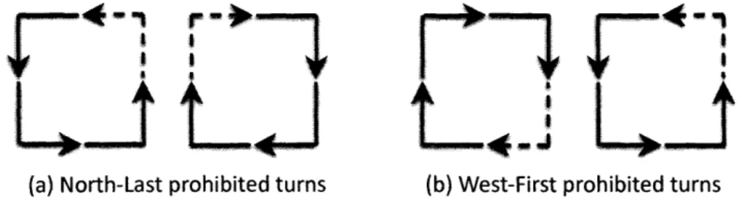
turn model [11] provides a few systematic approaches. Figure 3-2 illustrates some of these

approaches where the dotted segments represent the prohibited turns.1

For the 3 x 3 mesh network from Figure 1-2, the two acyclic CDGs derived from D 'Note that the turn model was developed to enable adaptive routing; here we are concerned with choosing routes in an offline fashion for oblivious routing.

(30)

using the north-last and west-first turn models shown in Figure 3-2 to break cycles are exhibited by Figure 3-3.

Cycles can also be broken in an ad hoc or random fashion as shown in Figure 3-4. Typically, a larger number of dependences need to be removed to obtain an acyclic CDG but after route selection under this type of CDG, we may obtain a better result (cf. Section

(a) North-Last prohibited turns (b) West-First prohibited turns

Figure 3-2: Two Turns Prohibited by the turn model. (a) North-Last turn. (b) West-First turn.

(a) North-Last based acyclic CDG (b) West-First based acyclic CDG

(31)

6). In both of the cases presented in Figure 3-4, 12 edges needed to be removed from the original CDG with no 180-degree turns, as opposed to 8 in the turn model. We can use

any acyclic CDG to drive our bandwidth-sensitive oblivious routing algorithm. Given that

different CDG's may result in different qualities of routes, we can perform route selection under many different CDG's and select the best result. We next show how to derive a flow network from an acyclic CDG so the routes generated are guaranteed to be deadlock-free.

3.4 Deriving a Flow Graph from an Acyclic CDG

Given source and destination network nodes si and ti respectively, for each flow i, we will derive a flow graph or network GA from an acyclic CDG DA. We will then run our route selection algorithm on GA, to find the "best" routes for the flows. This will have the effect of running route selection on the given flow network G (corresponding to the interconnection network) but with the route conforming to DA. If the routes for all flows conform to DA, deadlock freedom is assured.

Note that G corresponds to the original on-chip network, whereas GA corresponds to a flow network where the vertices are links of the original network, and the edges are

DC FA LF AF AB CB CB (b)B FL ic BC FE BE ED CD EH ILH LH CD ED EH DG HG DG HG GH GD GH OD HL DE HE LF AF F ) HE DE DC HL FE FL EF EB FA BA BA BC

(a)

(b)

(32)

dependences. We next focus on the route selection step.

GA is derived from DA as follows. DA is copied over to GA. Add vertices to GA corresponding to si and ti, for each i. Add edges from si to all vertices in GA that have si as the source node of the corresponding link. For example, if si is network node A in the 3 x 3 mesh network shown in Figure 1-2, then add edges from si to AB and AF. For each vertex in GA that has ti as the destination node of the corresponding link, add an edge from the vertex to ti. For example, if ti is network node I in the 3 x 3 mesh mesh shown in Figure 1-2, then add edges from FL to ti and from HL to ti.

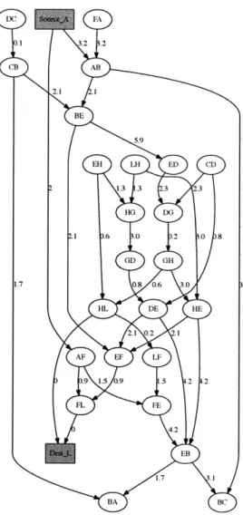
Figure 3-5 shows a flow network derived from the acyclic CDG of Figure 3-4(a), given the source-destination pair A, L. The weights on the edges are assigned randomly for illustration; their generation and utility will be described at a later stage. Other source-destination pairs can be added to GA in a similar fashion. Each link in GA will have an initial capacity and its residual capacity will change through the course of route selection. Both the MILP and the Dijkstra-based algorithm we use assume weights/capacities on edges. Each edge in G' has a capacity or residual capacity associated with the link vertex that it is incident on.

In this thesis we present two route selection schemes; an optimal route selector for some cost functions using mixed integer-linear programming. Solvers such as CPLEX are able to find optimal routes within a reasonable amount of time for moderate-sized examples, but not for large examples since the convergence time may be very long. To address this, we will also propose a heuristic algorithm for route selection based on Dijkstra's weighted shortest path algorithm [63].

3.5 Mixed Integer-Linear Programming Selector

Bandwidth allocation given the rate demands for each of the connections can be viewed as a multicommodity flow problem which can be optimally solved in polynomial time using linear programming (LP) [63]. The routes produced, using linear programming, are not by default deadlock free and can lead to splitting of flows. The mixed integer-linear program-ming (MILP) formulation below can produce an optimal result either minimizing maximum channel load, or maximizing throughput, therefore providing a way of selecting best routes for moderate-sized problems.

MILP: Find an assignment of flow in GA, i.e., Vi, V(u, v) E E fi(u, v) > 0, which satisfies the constraints:

Capacity constraints :

k

V(u, v) EE Zfi(u,v) < c(u,v) i= l

(33)

Figure 3-5: Flow network from acyclic CDG of Figure 3-4 with source-destination pair A, L and example weights.

Flow conservation:

Sfi(,

u

) =

(w,u)EE (u,w)EE( (u,w)eE

Vi

E

f(si, w) =

(si,w)EE Sfi (w, ti) = gi (w,ti)EE Unsplittable flow : fi(u, v) < bi(u, v) - di Vi, Vu E bi(u, v) < (u,v)EE Vi, Vu si , ti Vi , V(u, v) E E

(34)

Hop Count:

Vi b(u, v) < hopi

(u,v)EE

and minimizes the maximum channel load:

k

minimize U = max

f

(u, v) (3.2)

(u,v)EE

or maximizes the total throughput, given as

k

maximize S = gi (3.3)

i=1

or maximizes the minimal fraction of the flow of each commodity to its demand:

maximize T = min i (3.4)

1<i<k di

The variables bi(u, v) are Boolean variables, i.e., they can take on values of 0 or 1 only. They enforce the restriction that a flow i can only take a single path from source si to destination ti. They also enforce path length restrictions. hopi is a specified constant that can be set to be equal to the minimal path length between si and ti. This will imply that only minimal paths will be considered. hopi should be incremented by 2 or more to allow for non-minimal routing. The fi(u, v) variables can take on any positive value less than or equal to the demand di. Thus, we have a mixed integer-linear program, which if solved, finds the "best" set of routes, while ensuring unsplittable flows that conform to DA and are therefore deadlock-free.

3.6 Dijkstra Weighted Shortest Path Selector

Since the unsplittable flow problem is NP-hard even for single sources [19], MILP which is an approximation algorithm may not converge quickly enough to explore a good range of cycle breaking schemes and weight functions for large size problems. Therefore we present a heuristic for dealing with such cases, it consists of running Dijkstra on a weighted version of GA, deriving weights from the residual capacities of each link/vertex. Consider a link e in the original network G (e.g., AB) which is a vertex in GA. This link has a capacity c(e). We have a variable for each link e, called a(e), which is the current residual capacity of link e. Initially, it is equal to the capacity c(e). If a flow i is routed through this link e, we will subtract the demand di from the residual capacity a(e).

We have experimented with various metrics, and have selected the reciprocal of link residual capacity which is similar to the CSPF metric described by Walkowiak [54]. The

(35)

weight function we use is w(e) = a(e)-dj+M. c(e) is the current residual capacity that is decremented by di if the flow goes through e. c(e) may become negative when demands are higher than link bandwidths. M is a constant comparable to the maximum link bandwidth, large enough to ensure that the weights w(e) remain positive.

Dijkstra assumes weights on edges in GA; however, the links are vertices in GA. The weight of an edge in GA is merely the weight of the link/vertex that the edge is incident on. For example, the edge from si to AB will be assigned the weight of link/vertex AB. An edge from AB to BC will be assigned the weight associated with link/vertex BC. The edges incident on ti are always assigned a weight of 0. Figure 3-5 shows a flow network derived from the acyclic CDG of Figure 3-4(a), assuming the source is network node A and the destination is network node L, with weights assigned to edges. We run Dijkstra on the weighted GA to find a minimum weight path from A to L, or in general from an si to a ti. Then, the weights are updated, and a new source-destination pair is selected to be routed. This continues until all the flows have been routed.

This Dijkstra weighted shortest path based heuristic can be run on thousands of nodes within seconds. The underlying Dijkstra algorithm has polynomial-time complexity of

O(flows * (E + VlogV)).

This strategy results in a bandwidth allocation that tries to distribute traffic uniformly through the network, minimizing the maximum channel load. The length of the paths are minimized in a secondary fashion, since the weight of a path is the sum of the weights of the links. Increasing M gives more weight to minimizing the number of hops in each path, therefore providing a mechanism, like in the MILP based approach, to generate only minimal length routes for some applications where latency in terms of number of hops should be minimized.

3.7 Multiple Virtual Channels

Channel dependence graph representations of networks are expandable to networks with multiple virtual channels (VCs) per physical channel. Having multiple VCs per link does affect the deadlock properties of the network. Since resources in the network are no longer physical links but buffer spaces.

If there are z virtual channels per link in the network , then we expand the CDG D to include z vertices for each link, with each vertex corresponding to a virtual channel. There are edges between vertices if the corresponding links can be consecutively traversed by a packet. Since a packet can switch virtual channels, we will have z2 edges between the sets of vertices that correspond to consecutive links.

The CDG D for the 2 x 2 sub-mesh (with nodes F, E, A and B in the 3 x 3 mesh of Figure 1-2) for z = 2 is shown in Figure 3-6 (a).

(36)

As before, we can break cycles in D by removing edges using a strategy based on a turn model, or using ad hoc or random strategies. Figure 3-6(b) shows an acyclic CDG that was derived using a turn model.

We have additional flexibility with multiple virtual channels; all turns are allowed pro-vided the route switches virtual channels as shown in the acyclic CDG DA of Figure 3-6(c). Either (or both) of these acyclic CDGs can be used to generate the flow network GA by adding source and destination nodes as before. When a path pi is selected in GA, it implies a static allocation of virtual channels along the route. A best set of routes, i.e., the set with smaller maximum channel load, can be chosen across different acyclic CDGs. Therefore, static allocation of virtual channels gives additional flexibility in route selection. Shim et

al show in [53] that this type of static allocation can match or exceed the performance of

dynamic allocation schemes.

To evenly distribute flows across virtual channels, we modify the weight function slightly to include the number of flows that use a virtual channel. The weights of edges in G'A incident on ABO or AB1 will be different if ABO has been assigned to a flow, and AB1 has not.

Another approach, when we have a network with multiple VCs per physical channel, is to represent the network as multiple virtual networks. Each virtual network contains one or more virtual channels from the original network and it is represented by its own CDG (VCDG). Cycles in a VCDG are eliminated using either a turn or ad hoc model independently of other VCDGS. Given source and destination network nodes si and ti respectively, for each flow i, we will connect si and ti to all the acyclic VCDGS. Figure 3-7 shows a flow network derived from the 3 x 3 mesh network in Figure 1-2 with two virtual channels per link. Each virtual network has one virtual channel and the two virtual networks are shown

BA 0 BA 1 CDO 0 CDI

CB0 ABO CBI BC I

ADO ADI DA 0 DA 1

DC 0 DC 1 AB 0 AB 1

CB0 CB 1 BC 0 BCI ADO DAB

(a) (b) (c)

Figure 3-6: (a) CDG for 2 x 2 sub-mesh FEAB with 2 virtual channels (b) Acyclic CDG using the turn model. (c) Ad hoc Acyclic CDG.

(37)

in Figures 3-3(a) and 3-4(a). For illustration purposes, we have the source-destination pairs

sl = G, di = L.

Our routing scheme, by exploring virtual channel allocation based on application static information, helps prevent performance degradation associated with a single flow consum-ing multiple virtual channels and blockconsum-ing other flows, essentially eliminatconsum-ing the resource coupling created by the addition of buffers to the router architecture.

Both minimal and non-minimal paths can be selected in a bandwidth-sensitive manner

. : .- ---... ---...

LH 0 GH_0 DC1 FA 1

VD~ NelrVC 0 ViFA NeGH_1 rVGD 1

E C0 DE1 AHE1 B HL 1

A 0 ELF 1 AF_1 EF_1

EF 0

----

H 0-

----

ED 0

--

---

FEG1

_

FL 1

FL 0 DG 0 EB 1

BA 1 BC 1

(38)

in our framework, while ensuring that deadlock does not occur. Hardware restrictions such as limiting the number of flows through a link can be enforced when searching for a new route. Many different acyclic CDGs and cost functions can be used in an effort to obtain the best performance as determined by a simulator or router hardware. Packet routes can be determined in different orders. Finally, other route selectors can be plugged into the framework rather than using MILP or Dijkstra as long as required deadlock-avoidance checks on the set of routes are made.

(39)

Chapter 4 Router Architecture

This chapter discusses the impact of our oblivious routing technique on the router archi-tecture, and compares the modified architecture with standard routers for other oblivious routing algorithms. The following discussion assumes a typical virtual-channel router on a two-dimentional mesh network as a baseline. However, as previously noted the proposed routing technique is largely independent of network topology and flow control mechanisms. Therefore, the same approach to routing can be applied to other network topologies and

either packet-buffer or flit-buffer flow control.

4.1 Typical Virtual Channel Router

---VC state

nput Output

• .Switch Allocation

• (SA)

Input VCstate Output

SPortSwitch Traversal

(a) Router architecture (b) Router pipeline

Figure 4-1: Typical virtual-channel router architecture. The dark blue indicates that the modules and pipeline stages may be modified for our approach.

(40)

Routing algorithm Routing mechanics VC allocation DOR, ROMM, etc. Algorithmic: fixed logic Dynamic

BSOR / No Cycle (NC) Table-based: source or node-table routing Dynamic or Static

Table 4.1: Router architecture designs for routing algorithms.

Figure 4-1 illustrates a typical virtual-channel router architecture and its operation [24, 27, 39]. As shown in the figure, the datapath of the router consists of buffers and a switch. The input buffers store flits while they are waiting to be forwarded to the next hop. There are often multiple input buffers for each physical channel so that flits can flow as if there are multiple "virtual" channels. When a flit is ready to move, the switch connects an input buffer to an appropriate output channel. To control the datapath, the router also contains three major control modules: a router, a virtual-channel (VC) allocator, and a switch allocator. These control modules determine the next hop, the next virtual channel, and when a switch is available for each packet/flit.

The routing operation takes four steps, namely routing (RC), virtual-channel allocation (VA), switch allocation (SA), and switch traversal (ST), which often represent four pipeline stages in modern virtual-channel routers. When a head flit (the first flit of a packet) arrives at an input channel, the router stores the flit in the buffer for the allocated virtual channel and determines the next hop for the packet (RC stage). Given the next hop, the router then allocates a virtual channel in the next hop (VA stage). Finally, the flit competes for a switch (SA stage) if the next hop can accept the flit, and moves to the output port (ST stage).

For existing oblivious routing algorithms such as Dimension Ordered Routing (DOR) [1], ROMM [16], Valiant [8], and olturn [46], the next hop of a packet can be easily computed at each router node based on the packet's destination. Moreover, these algorithms are fixed and commonly used for all types of applications and traffic patterns. As a result, traditional oblivious routing algorithms are implemented as dedicated logic in the RC stage of each router. For these routing algorithms, the RC stage is quite simple and the router frequency is typically dominated by the VA stage [24].

4.2 Router Architecture for Bandwidth-Sensitive Oblivious

Routing (BSOR)

The router architecture for the proposed oblivious routing scheme is almost identical to the typical virtual-channel router architecture. The router uses the exact datapath that is described above. The only change in our routing architecture is in its routing module, which is summarized in Table 4.1.

Application-aware deadlock-free oblivious routing

Application-Aware Deadlock-Free Oblivious Routing

by

Michel A. Kinsy

Submitted to the Department of Electrical Engineering and Computer Science

in partial fulfillment of the requirements for the degree of

Master of Science in Electrical Engineering and Computer Science

at the

MASSACHUSETTS INSTITUTE OF TECHNOLOGY

ARCHIVES

June 2009

@

Massachusetts Institute of Technology 2009. All rights reserved.

Author ... ...

...

Department of Electrical Engineering and CompL /Science

May 11, 2009

(n

Certified by ...

Srinivas Devadas

Professor of Electrical Engineering and Computer Science

Thesis Supervisor

Accepted by ...

Terry P. Orlando

Chairman, Department Committee on Graduate Students

Department of Electrical Engineering and Computer Science

AUG 07RI ES2009

LIBRARIES

Application-Aware Deadlock-Free Oblivious Routing

Acknowledgements

Contents

List of Figures

List of Tables

Chapter 1

Introduction

1.1

Topology of Networks-on-chip

1.2

Message Flow Control in Networks-on-chip

1.3

Network Resource Interface

1.4

Routing in Networks-on-chip

1.5

Contributions

1.6

Organization

Chapter 2

Background and Related Work

2.1

Oblivious Routing Algorithms

2.2

Application-Specific Routing Algorithms

yt

2.3

Buffer Space and Bandwidth Allocation

2.3.1

Buffer Space Allocation

2.3.2

Bandwidth Allocation

(b)

2.4

Adaptive Routing Algorithms

Chapter 3

Oblivious Routing with Bandwidth

Sensitivity

3.1

Definitions

f

3.2

BSOR Framework

3.3

Creating Acyclic Channel Dependence Graphs

3.4

Deriving a Flow Graph from an Acyclic CDG

(a)

(b)

3.5

Mixed Integer-Linear Programming Selector

Sfi(,