Lessons learned from developing turbulence profilers for telescopes' instruments Lessons learned from developing turbulence profilers for telescopes' instruments

(1)

HAL Id: hal-01232590

https://hal-amu.archives-ouvertes.fr/hal-01232590

Submitted on 23 Nov 2015

HAL is a multi-disciplinary open access archive for the deposit and dissemination of sci-entific research documents, whether they are pub-lished or not. The documents may come from teaching and research institutions in France or abroad, or from public or private research centers.

L’archive ouverte pluridisciplinaire HAL, est destinée au dépôt et à la diffusion de documents scientifiques de niveau recherche, publiés ou non, émanant des établissements d’enseignement et de recherche français ou étrangers, des laboratoires publics ou privés.

Lessons learned from developing turbulence profilers for

telescopes’ instruments Lessons learned from developing

turbulence profilers for telescopes’ instruments

Andrés Guesalaga, Benoit Neichel, Clémentine Béchet, Javier Valenzuela

To cite this version:

Andrés Guesalaga, Benoit Neichel, Clémentine Béchet, Javier Valenzuela. Lessons learned from de-veloping turbulence profilers for telescopes’ instruments Lessons learned from dede-veloping turbulence profilers for telescopes’ instruments. Journal of Physics: Conference Series, IOP Publishing, 2015, 595 (012013). �hal-01232590�

(2)

This content has been downloaded from IOPscience. Please scroll down to see the full text.

Download details:

IP Address: 147.94.212.92

This content was downloaded on 23/11/2015 at 16:09

Please note that terms and conditions apply.

Lessons learned from developing turbulence profilers for telescopes’ instruments

View the table of contents for this issue, or go to the journal homepage for more 2015 J. Phys.: Conf. Ser. 595 012013

(http://iopscience.iop.org/1742-6596/595/1/012013)

(3)

Lessons learned from developing turbulence profilers for

telescopes’ instruments

Andrés Guesalaga1_{, Benoit Neichel}2_{, Clémentine Béchet}1_{, Javier Valenzuela}3,1

1_{Universidad Católica de Chile, Vicuna Mackenna 4860, Santiago, Chile} 2_{LAM, Rue Frederic Joliot Curie, 13013 Marseille, France}

3_{European Southern Observatory, Alonso de Córdova 3107, Vitacura, Chile} E-mail: [email protected]

Abstract. This article presents the results obtained during three years of developing turbulence profilers for two different telescopes; namely Gemini South and the future Adaptive Optics Facility (AOF). The profilers are embedded in a facility instrument that provides the data from the Shack-Hartmann wavefront sensors which feed the SLODAR approach used to generate the profiles. The main results focused on two unsolved problems: dealing with the dome seeing and the effect of the atmosphere outer scale on the accuracy of the profilers.

1. Introduction

The performance of wide-field Adaptive Optics (AO) system is expected to be optimized with a good knowledge of the vertical distribution of the turbulence strength in the atmosphere [1]. As the first laser-based conjugate AO system offered to the astronomers community, GeMS (Gemini Multi-conjugate AO system) has already started to study two different methods for the estimation of the Cn2 profile out of its AO telemetry [2]. These two techniques rely on the Slope Detection and Ranging (SLODAR) approach [3], using the cross-covariances of simultaneous wavefront sensor measurements each pointing at a different guide star in the field of view. In previous works, the SLODAR methods have been adapted to account for the cone effect when using laser guide stars (LGS) [2,4]. This leads to the estimation of the Cn2_{profile over a non-equally discretized representation of the vertical} turbulence distribution. The two methods have already been successfully used on GeMS telemetry recorded during the 2011, 2012 and 2013 campaigns [2,5,6]. A statistical analysis of these results has also been addressed in a recent paper [6]. We study the application of previous work to a new AO configuration, defined by the operating modes of the Adaptive Optics Facility (AOF) at the Very Large Telescope (VLT, Paranal Observatory of ESO). The AOF consists of an evolution of one of the VLT unit telescopes to a laser driven adaptive telescope with a deformable secondary mirror and four LGSs [7]. Because of its wide-field and tomographic AO modes, ESO is studying how to integrate one of this profiling technique into the AOF.

2. Results at Gemini

2.1. Profiling and dome seeing

In the literature, two different approaches have been used to analyse the data from SLODAR optical triangulation [2]. The first approach deduces the Cn2_{and wind profiles from the deconvolved} spatio-temporal cross-correlations of the. The second one does not apply such deconvolution, but rather

Adapting to the Atmosphere Conference 2014 IOP Publishing Journal of Physics: Conference Series 595 (2015) 012013 doi:10.1088/1742-6596/595/1/012013

Content from this work may be used under the terms of theCreative Commons Attribution 3.0 licence. Any further distribution

of this work must maintain attribution to the author(s) and the title of the work, journal citation and DOI.

(4)

models the spatial covariances of the slopes using a specific turbulence statistics (e.g. Kolmogorov or von Kármán): the turbulent layers heights and strengths are recovered by fitting theoretical impulse response functions to the cross-covariance of the slopes measurements.

These impulse response functions express how a theoretical turbulent layer located exactly at the centre of a bin corresponds to the measured slope covariance functions.

Essential elements in this method are the auto-correlation submaps. They not only provide an estimate of the measurement noise, but also give an idea of how well the data matches the theoretical statistics (usually Kolmogorov or von Kármán) used to generate the theoretical submaps. The central point of the auto-correlation submaps corresponds to the centroid from each subaperture correlated with it. As the measurement noise is fully correlated at the central point of this submap, this component will be the sum of the slope and the noise variances. Hence, the difference between the central points of the theoretical and measured auto-correlation submaps (Fig. 1) gives an estimate of the noise variance.

noise

Figure 1. Central slice of the X-slopes submaps in the Y direction. The solid line is the measured covariance and the dashed line in the theoretical impulse function. The difference in the central pixel corresponds to noise (data from April 15th, 2011).

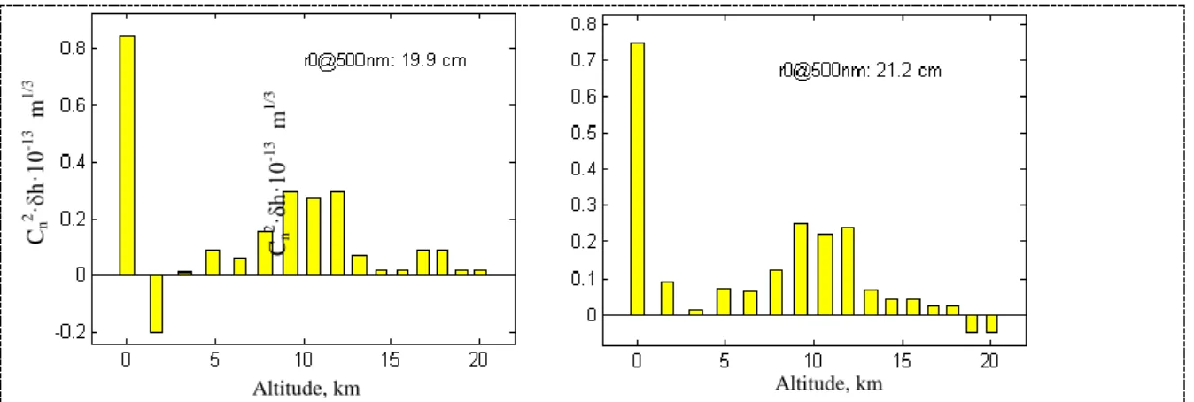
In many cases encountered with GeMS data, the profiles obtained by the model fitting and the deconvolution approaches differed similar to the ones shown in Fig. 2. The model fitting method produces a relatively strong negative Cn2_{at the bin immediately above the one at 0km. On the} contrary, the estimation by deconvolution from measured autocorrelation do not exhibits such unrealistic estimate. This point is of major importance to define which estimation approach is the most adequate for our objective, and we discuss here the reasons for such discrepancy.

During the two-year measurement campaign, strong dome seeing conditions were detected in a significant number of cases (~ 30% of the recorded conditions). Fig. 2 (left) shows an example of the slope variance in the X direction for the five WFSs after static aberrations were removed. The brighter pixels correspond to the subapertures with abnormally high variance that in this case was explained by turbulence behind the secondary mirror. Such strong dome seeing typically narrows the auto-covariance impulse response as shown in Fig. 2 (right panel). A clear departure from the theoretical shape (crosses) is observed for the measured function (continuous line) with a noticeable “elbow” around the third component off the centre.

Turbulence models such as von Kármán (finite outer-scale values) or Kolmogorov only account for the atmospheric turbulence and not for the non-Kolmogorov turbulence inside the dome. Trying to fit the measured covariance submaps to these theoretical statistical models can lead to erroneous profile estimations. Figure 3 (left) provides an example of such case where a strong negative value in the turbulence intensity appears at lower altitudes. A common characteristic of such disturbances is that they simultaneously show up in the same subapertures in all five WFSs, so the effect is the same as turbulence at the ground, making the estimation of the lower bins particularly sensitive to this effect. On the other hand, the use of the deconvolved cross-correlation implicitly accounts for the contribution of dome turbulence as the deconvolution function in equation (3) is constructed from the actual measurements. When this dome contribution is large, a narrower convolution function is obtained, leading to realistic estimates of the lower layers. However, this autocorrelation function also

(5)

includes the turbulence from the upper layers, which should behave closer to Kolmogorov statistics. This is our understanding of the degraded layer strength estimations for the upper layers.

The approach based on the deconvolved temporal cross-correlation has been extensively tested in several campaigns during 2011, 2012 and 2013.

Cn 2 ·δh ·1 0 -13 m 1/3 Altitude, km Altitude, km Cn 2 ·δh ·1 0 -13 m 1/3

Figure 2. Estimation using the model fitting (top) and the deconvolved cross-correlation (bottom) methods. The former shows a higher value at the first bin and a negative estimation at the second, due to non-Kolmogorov turbulence (data from November 4th, 2012)

Figure 3. Left: variance of the subaperture slopes in X direction for the 5 WFSs. Right: central slices of the auto-covariance response in X direction for a theoretical Kolmogorov (dotted) and measured (continuous line) turbulences. Notice the “elbow” forming around the ± 2 components in the abscissa (data from December 16th_{, 2011).}

2.2. Frozen flow decay (“melting”)

Using temporal correlation sequences, the layers can be tracked and their speed and direction estimated. As the individual correlation peaks are being tracked, the degree of correlation can also be computed, providing an estimation of the evolution of the layer, i.e. the correlation decay or the rate of ‘melting’ as it crosses the telescope’s field of view.

By selecting cases where the turbulence layers can be clearly isolated and tracked we focus on the analysis and interpretation of the observed dynamics of the turbulence intensity. In particular, we have estimated the rate of de-correlation of the layered turbulence as it passes over the telescope. Data collected in observation campaigns during 2011 through 2013, allowed us to gather about 74 sequences of turbulence layers where their decay rate could be determined. The set includes different conditions of altitudes, strength and velocities. In the case of the wind speed, their values ranged from 0 m/s for strong dome seeing conditions (9 cases) to speeds up to 24 m/s.

(6)

In the following analysis, we estimate the rate of de-correlation by: i) tracking the correlation peaks; ii) computing the correlation energy around the maximum. A 3x3 window is used for layers above the first bin. For the first bin (ground and dome), only the central pixel is considered; iii) normalizing the correlation values to the first correlation result in the sequence (peak at t = 0s).

As mentioned before and exemplified in Fig. 3, turbulences inside the dome are fairly common during operation of large telescopes. We have found that this type of turbulence remains stationary with zero translation velocity. The dome turbulence is spatially located in the same place in all WFSs, so it is seen as a layer at the ground. Hence, the profiler assigns its energy to the first bin and as this phenomenon is quasi static a distinctive stationary peak will appear during the temporal correlation sequence.

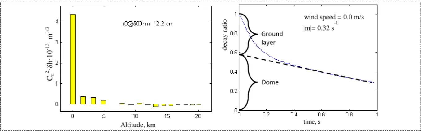
Fig. 4 (left) shows the profile for strong dome turbulence and in the right panel, the intensity of the central pixel in the sequence of time delayed correlation is shown. The plot (normalized to its value at

t = 0) shows a rapid initial decay, that gradually stabilizes to a rate of 0.32s-1_{. This fast initial decay} was found to be caused by a ground layer passing over the telescope that at the start of the temporal correlation is merged with the dome seeing. As time passes, this part of the turbulence moves away from the central peak so its correlation with the fixed frame is lost, but the dome turbulence will evolve much slower, maintaining a positive match for a longer time. By measuring the slope of the asymptotic dashed line, an estimate of the rate of de-correlation can be found.

Ground layer Dome wind speed = 0.0 m/s |m|= 0.32 s-1 Cn 2·δh· 10 -13 m 1/3 Altitude, km time, s d ec ay r atio Ground layer Dome wind speed = 0.0 m/s |m|= 0.32 s-1 Cn 2·δh· 10 -13 m 1/3 Altitude, km time, s d ec ay r atio

Figure 4. Left: turbulence profile in altitude, showing a strong component at the ground layer; Right: decorrelation rate of turbulence inside the dome (dashed line) and separation from the ground layer turbulence above the telescope (data from November 7th, 2012)

Wind speed = 21.3 m/s Wind direction = 227.7° |m|= 3.26 s -1 Cn 2 ·δh ·1 0 -13 m 1/3 Altitude, km d ec ay r atio time, secs Wind speed = 21.3 m/s Wind direction = 227.7° |m|= 3.26 s-1 Cn 2·δh ·1 0 -13 m 1/3 Altitude, km d ec ay r atio time, secs

Figure 5. Left: profile for a turbulence between 11.9 and 13.2 Km from data of April 17th, 2013; Right: estimation of the turbulence melting rate (dashed line)

The profile in Fig. 5 (left panel) presents a typical case of a strong layer in the jet stream at an altitude of around 12 Km. The measured speed is 21.3 m/s with a decay ratio of 3.26 s-1_{. A steeper decay in the} cross-correlation is observed in this case when compared to the previous cases (Fig. 5, right panel).

(7)

An interesting result of this turbulence “melting” rate comes from an integrated analysis for several cases. Fig. 6 plots the relative decay ratios against wind speed under different turbulence conditions and time. The data for this analysis were collected at Gemini South during the last two years.

A clear pattern can be observed between the dissipation rate and the wind speed with a remarkable resemblance to a linear dependence. Fitting a linear function to the set of points gives a slope of about -6.4 m-1_{. This suggests that the ‘melting’ of the turbulence for short time scales, depends on the} distance travelled rather than speed or altitude.

Fig. 6 highlights that many layers have been found with decay rate between -1 s-1_{and -3 s}-1_. Considering for instance a layer with a decay rate of -2 s-1_{, which occurs for a wind speed around} 10m/s, the correlation of this layer with the shifted one that occurred 250ms earlier (more than 125 AO cycles) still contains half of the energy in the original correlation peak. For all the cases presented in Fig. 7 the decay rate is smaller than -5 s-1_{, meaning that the correlation decreases by a factor lower} than 2 after 100ms, i.e. more than 50 cycles of the GeMS AO loop.

wind speed, m/s d ec ay r atio y = -0.157x – 0.365

Figure 6. Rate of decay in the cross-correlation of slopes with a clear linear dependence between wind speed and turbulence correlation decay. The slope of the linear fit is in m-1, suggesting that this de-correlation can be expressed in terms of the distance travelled by the layers across the pupil.

3. Results in the AOF

In this section, the profiling methods are applied on slopes sequences simulating the GALACSI wide-field mode (WFM) configuration [7].

3.1. Outer scale influence

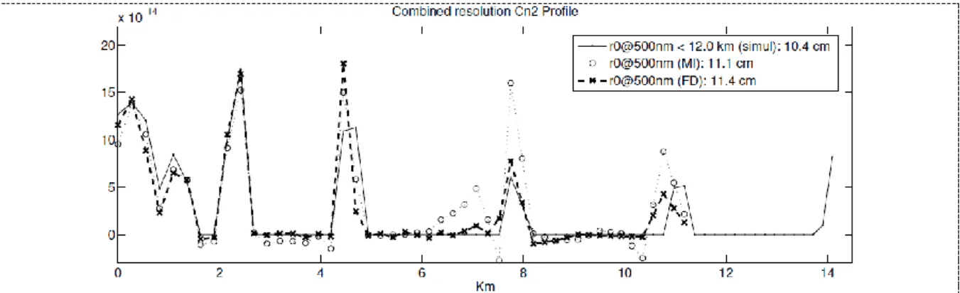
The turbulence strength, characterized by the Fried parameter r0, can be different for each layer, but the outer scale L0 for a von Karman model is used as a common value. In previous studies of these profiling methods on Gemini South LGS system, GeMS, a large outer scale of 150 m was used, being almost equivalent to assuming a Kolmogorov model as seen from the 8-meter aperture of the telescope [2,5]. In the standard case of GALACSI WFM presented above, if such an outer scale L0 = 150 m is assumed instead of the true value L0 = 25 m, the resulting profiles are the ones shown in Fig. 7.

Fig. 7 shows that the error on the outer scale assumption leads to major error in the estimation of the r0. The MI estimation of r0 is wrong by 6.3%, and the one provided by the FD method is erroneous by

9.9%. The correlation criterion for the MI method drops to 88% and to 92.5% for FD. Note also that the MI method produces negative values of much greater magnitude, than in Fig. 7. Although the general profiles patterns seem quite similar as in Fig. 7, a significant difference appears for the altitude layer at 7.75 km in the case of the MI method. On its side, the FD method provides modified values compared to Fig. 7 overall for the lowest layers, but not significantly for the higher ones. While the MI really seems to detect a false layer at 7 km, the FD profile is not affected in this region.

The results of Fig. 7 highlight the importance of a correct

L

0 assumption to properly estimate r0 and

the relative profile. Therefore, in this section, the influence of the outer scale assumptions on the

(8)

profilers is studied more extensively, showing by how much it can impact the r0 estimate and the profile distribution.

Figure 7. Same telemetry data is used as in Fig. 1, but the profiling methods are setup assuming an outer scale L0 = 150 m instead of the true value L0 = 25 m.

GALACSI wide field mode have been simulated with the same random seed, the same noise, but changing the value of the atmosphere outer scale

L

0simulation. For the registered data telemetry out of

these simulations, the profilers have been applied assuming different values of outer scale

L

0 and

enhancing the influence of the latter on the result.

The estimation of r0 is presented for MI method on the left and for FD method on the right. When the

outer scale value of simulated atmosphere,

L

0simulation matches the outer scale

L

0 assumed in the

structure function for a profiling method, it is observed that the error on r0 is only a few percent points when the assumed outer scale is correct. For atmospheres with short outer scale, the MI method is very sensitive to the assumed

L

0 value. An overestimation of L0 can make the error jump to almost 100%

of error. For the FD, the largest errors observed on r0 are not so important, but still reach 25% error.

The quality of the profiling method cannot only be summarized by the error r0. The correlation factor is used again on the similarity of the simulated outer sale

L

0simulation and the value of

L

0assumed in the

each method. This provides a complementary assessment of the profiling method for which we expect to get the maximum correlation when

L

0simulation =

L

0. It is observed that for the range of outer scale

considered in the simulations, the correlation stays greater than 80% for the MI method and greater than 90% for the FD one. Together with these results a superior performance of the FD method can thus already be highlighted. This last method is less sensitive to a wrong assumption on the outer scale value, but can still lead to significant error on r0.

3.2. Finding a good L0

The results in the previous section raise the problem of a good agreement between the real atmosphere outer scale and the assumed value in the profilers. A one-dimensional representation of these theoretical auto-covariance functions, normalized to their maximum, is illustrated on the left of Fig. 9. The various curves reveal how the outer scale L0 affect the shape of the auto-covariance, from L0 = 3 m to L0 = 150 m. Actually, on this plot, the curves for L0 = 100 m and L0 = 150 m cannot be distinguished, meaning that the response of the system is practically the same for a Kolmogorov turbulence or for a von Karman one with outer scale greater than 100 m. For shorter outer scales, the shape of the auto-covariance varies with L0.

The fitting is made using the 5x5 central sampled values of the autocorrelation except the central point which is the variance of the slopes in a subaperture. This variance value computed from the telemetry is affected by the noise measurement and thus is not used for the fit to the theoretical autocovariance function. The L0 value producing the least weighted square error is kept for the L0 assumption when applying the profiling methods. It has been checked that this simple approach is able to properly identify the outer scale value in all the diverse simulations that have been run for this study. An

(9)

example is shown on the right of Fig. 10, where the measured autocovariance (line with crosses) for an AO simulation of GALACSI WFM with an average LGS flux of 40 photons per subaperture per frame and an outer scale L0simulation = 25 m is compared to its best fitted autocovariance (line with squares).

Figure 8. Left: Autocovariance functions obtained for the GALACSI WFM configuration and normalized to their maximum value. The various curves stand for varying outer scales ranging from 3 to 150 m.

4. Further work and conclusions

As highlighted in the paper, the correct assumption on the outer scale is crucial in order to estimate properly the Cn2_{distribution and the r}

0 of the atmosphere. The outer scale fitting method presented above in that sense constitutes a key element to be included in the algorithms. Nevertheless, previous experience with on-sky data taken by GeMS instrument revealed the significant probability to face dome seeing or a particular turbulence contribution which would have a different outer scale than the rest of the atmosphere. In such case, the assumptions made on the turbulence model do not apply anymore and both methods are expected to provide degraded estimations of the Cn2_{profiles and r}

0. It remains for further work to find a way to take into account various outer scale at different heights. Such improvement of the profiling method is currently studied for the MI approach, for which it is expected to be easier to enlarge the matrix model including impulse response to various outer scale values.

Acknowledgments

This work was supported by the Chilean Research Council (CONICYT) grant Fondecyt 1120626 References

1. T. Fusco and A. Costille, Impact of Cn2 profile structure on wide-field AO performance, in Adaptive Optics Systems II, 7736, pp. 77360J, 2010.

2. A. Cortes, B. Neichel, A. Guesalaga, J. Osborn, F. Rigaut, and D. Guzman, Atmospheric turbulence profiling using multiple laser star wavefront sensors, MNRAS 427, pp. 2089-2099, Dec. 2012.

3. R. W. Wilson, Slodar: measuring optical turbulence altitude with a Shack-Hartmann wavefront sensor, MNRAS 337(1), pp. 103-108, 2002.

4. L. Gilles and B. L. Ellerbroek, Real-time turbulence profiling with a pair of laser guide star shack-hartmann wavefront sensors for wide-field adaptive optics systems on large to extremely large telescopes, J. Opt. Soc. Am. A 27, pp. A76-A83, Nov 2010.

5. A. Guesalaga, B. Neichel, A. Cortes, C. Bechet, and D. Guzman, Using the Cn2 and wind profiler method with wide-field laser-guide-stars adaptive optics to quantify the frozen-flow decay, MNRAS 440(3), pp. 1925-1933, 2014.

6. I. Rodriguez, B. Neichel, C. Bechet, D. Guzman, and A. Guesalaga, Statistics of atmospheric turbulence at Cerro Pachon using the GeMS profiler, SPIE, 2014.

7. R. Arsenault, P.-Y. Madec, J. Paufique, et al, “ESO adaptive optics facility progress report," SPIE 8447, 2012.