Publisher’s version / Version de l'éditeur:
Vous avez des questions? Nous pouvons vous aider. Pour communiquer directement avec un auteur, consultez la première page de la revue dans laquelle son article a été publié afin de trouver ses coordonnées. Si vous n’arrivez pas à les repérer, communiquez avec nous à [email protected].
Questions? Contact the NRC Publications Archive team at
[email protected]. If you wish to email the authors directly, please see the first page of the publication for their contact information.
https://publications-cnrc.canada.ca/fra/droits
L’accès à ce site Web et l’utilisation de son contenu sont assujettis aux conditions présentées dans le site LISEZ CES CONDITIONS ATTENTIVEMENT AVANT D’UTILISER CE SITE WEB.
Research Report (National Research Council of Canada. Institute for Research in
Construction), 2009-03-02
READ THESE TERMS AND CONDITIONS CAREFULLY BEFORE USING THIS WEBSITE. https://nrc-publications.canada.ca/eng/copyright
NRC Publications Archive Record / Notice des Archives des publications du CNRC :
https://nrc-publications.canada.ca/eng/view/object/?id=474d480e-3057-47e4-baa1-e4664b5c1768
https://publications-cnrc.canada.ca/fra/voir/objet/?id=474d480e-3057-47e4-baa1-e4664b5c1768
Archives des publications du CNRC
For the publisher’s version, please access the DOI link below./ Pour consulter la version de l’éditeur, utilisez le lien DOI ci-dessous.
https://doi.org/10.4224/20373943
Access and use of this website and the material on it are subject to the Terms and Conditions set forth at
Verification and validation: establishing confidence in hygrothermal
tools
Confidence in Hygrothermal Tools
National Research Council of Canada
Institute for Research in Construction
Research Report IRC-RR-278
Authors: Steve Cornick
Research Officer
Wahid Maref
Research OfficerFistum Tariku
Technical OfficerDate: May 4, 2009
Pages: 21
Table of Contents
ABSTRACT ... 4
INTRODUCTION... 4
VERIFICATION ... 5
An Analytical Exercise ... 5
Time step dependency ... 5
Grid dependency ... 6
Error Analysis ... 6
A Common Exercise ... 8
Error Analysis ... 8
Grid dependency ... 8
Time step dependency ... 9
VALIDATION ... 9 Laboratory Testing ... 12 Field validation ... 13 DISCUSSION ... 16 CONCLUSIONS ... 18 ACKNOWLEDGEMENTS ... 18 REFERENCES ... 19
List of Figures
Figure 1 – Summary of construction, initial and boundary conditions for the analytical exercise ... 5Figure 2 – Moisture content profile in % through the layer at 1000 hours. The analytical solution is also included. The x-value through the layer has been normalized. ... 6
Figure 3 – Moisture content profile in % through the layer at 1000 hours. The analytical solution is also included. The x-value through the layer has been normalized. ... 7
Figure 4 – External and internal climatic loads (SI top and I-P bottom). Heat load from exterior is given in terms of differences between external equivalent, Teq,a, and external air temperature Ta. Moisture load on the external side is given as a rain flux and vapour pressure, and on the internal side as the vapour partial pressure, ps,i at a constant temperature (adapted from Hagentoft et al. 2003)... 10
Figure 5 – Moisture content profile of the outer surface for the duration of simulation. The accepted solution is the average result of an inter-model comparison, CI+ and CI- the upper and lower 99.9% confidence limits. ... 11
Figure 6 – Moisture content profile through the structure at hour 96 of the simulation. The accepted solution is the average result of an inter-model comparison, CI+ and CI- the upper and lower 99.9% confidence limits. The x-value through the layer has been normalized. ... 11
Figure 7 – Percentage error between predicted and measured total moisture contents for the OSB layers for all four walls tested. ... 14
Figure 8 – Statistical errors for all the wall sets. Mean absolute, mean bias, root mean squared error. RMSE systematic and unsystematic errors are also shown. ... 14
Figure 9 – Effect of changing the water vapour permeance. The average OSB properties are compared with the measured properties of a 10.1 mm sheet of OSB and a 20% variation in water vapour permeance. ... 15
Figure 10 – Comparison of measured and computed relative humidity at the outer section. Three scenarios are shown; 1) reported values and default coefficients, 2) a low MTC, and 3) an elevated indoor RH. ... 16
Figure 11 – Comparison of measured and computed relative humidity at the middle section. Three scenarios are shown; 1) reported values and default coefficients, 2) a low MTC, and 3) an elevated indoor RH. ... 17
Figure 12 – Comparison of measured and computed relative humidity at the inner section. Three scenarios are shown; 1) reported values and default coefficients, 2) a low MTC, and 3) an elevated indoor RH. ... 17
List of Tables
Table 1 ... 8 Correlation coefficient, x,y, and F-test for the simulation and analytical solutions at 100, 300, and 1000
hours; 13 node one hour time step case. ... 8 Table 2 ... 9 Grid variations for common exercise. Rows are for a particular grid. Numbers indicate the numbers of
nodes per layer. ... 9 Table 3 ... 17 Statistical errors for all the wall sets; Mean absolute, mean bias, root means squared error. RMSE
systematic and unsystematic errors are also given as well as the correlation coefficient and F-Test statistic. ... 18
Verification and Validation: Establishing
Confidence in Hygrothermal Tools
Steve Cornick
1*, Wahid Maref
1, and Fitsum Tariku
2ABSTRACT
The hygrothermal performance of building envelope systems is dictated by their responses to combined heat, air and moisture fluctuations produced by exterior and interior conditions. Research has focused on both laboratory experimentation and modeling of envelope systems by computer programs (hygrothermal tools). Experimental studies played a crucial role in the development of hygrothermal tools, and continue to offer useful information for their improvement. To be used with confidence, however, hygrothermal tools must be verified and, if possible, validated. To date, no comprehensive schemes for benchmarking hygrothermal tools exist as, for example, exist for energy simulation tools. Three comparisons are typically used to show the practical merits of simulation tools: inter-model, analytical, and empirical. This paper demonstrates how confidence in a 1-dimensional hygrothermal simulation tool can be built by such comparisons, and proposes them as the basis for a verification and validation methodology.
INTRODUCTION
Although modeling heat air and moisture through envelopes has been developed to the point where commercially available tools are available to practitioners other state-of-the-art hygrothermal modeling (HAM) tools have not reached the state of maturity that other simulation tools, such as those for energy, have reached. Even though the governing equations are well understood (Hagentoft et al. 2003; Tariku 2007), there are several reasons for this for lack of development. First is the expanding nature of the problem. Whereas practitioners can use modeling tools with some degree of confidence to investigate the hygrothermal behaviour of one or two-dimensional model walls in isolation; the current trend in model development is towards a holistic approach that couples the response of the wall with the behaviour of the space it encloses (Tariku 2008; Woloszyn and Rode 2008a; Holm and Lengsfield 2007; Salonvaara et al. 2003; Salonvaara and Karagiozis 1999; Rode and Woloszyn 2007). Considerable work remains to adequately couple ventilation, energy, and hygrothermal simulation models. Although there are now commercially available tools the guidance for using them is limited. Standards such as 160-2009 (ASHRAE 2009) offer guidance to the practitioner when considering moisture in the envelope design process. However, these standards are under development and several issues are still being resolved, for example the selection of proper interior and exterior boundary conditions (Cornick et al. 2003; Cornick and Kumaran 2008; Cornick and Dalgliesh 2008; ASHRAE 1325-RP). More fundamentally, the determination of appropriate moisture transfer coefficients is of importance, especially given the trend towards holistic modeling (Neale et al. 2007a, 2007b). Finally the selection of materials and the determination of material properties is an area of continuing research (Mukhopadhyaya et al. 2007; Holm and Hartwig 2002; Karagiozis and Salonvaara 1995).
When using simulation tools to investigate the performance of the building envelope, a good understanding of the capabilities and limitations of the tool being used is also crucial. Beyond the balance equations, there are other aspects and assumptions that, if a user is aware of and understands them, can be used of to produce better results. Confidence in the tool is key. Confidence is gained through a process sometimes called „benchmarking‟, though verification and validation are more correct terms. For energy simulation tools, there are well-established procedures for establishing confidence in simulation tools (ASHRAE 2004), but this is not the case for hygrothermal simulation tools. One project, HAMSTAD (Hagentoft et al. 2003), involved round-robin testing of different hygrothermal tools from around the world.
1
Research Officer, Institute for Research in Construction, National Research Council Canada *
Corresponding author 2
Director of Building Science Centre of Excellence, School of Construction and Environment, British Columbia Institute of Technology
A series of exercises was developed to establish confidence in newly developed one-dimensional programs, by testing them against analytical problems or by inter-program comparisons of more complex problems. Recently a series of common exercises designed to test whole building models has been published as part of the completion of IEA Annex 41 (Woloszyn, M. and C. Rode 2008b.)
The work presented here draws heavily on work reported elsewhere; specifically the benchmarking of a 1- and 2-dimensional hygrothermal tool (Maref et al 2004b, Cornick 2006, Tariku and Kumaran 2006). Most of the previous work was done using an in-house research 2-D hygrothermal simulation tool. That work was repeated, this time, however, using a publicly available 1-D hygrothermal tool (Maref et al. 2004a; Cornick 2006) with modification of any sort; “out of the box” as it were. The objective of this paper is to explicate the process of verification and validation in order to demonstrate the development of a methodology that could serve as a basis for a standard similar to ASHRAE 140 Standard Method of Test
for the Evaluation of Building Energy Analysis Computer Programs (Judkoff and Neymark, 2006).
VERIFICATION
Verifying modeling tools consists of ensuring that the physics incorporated in the tool has been
implemented correctly. According to ASHRAE 140, the process of verification applied to software means essentially testing the software to ensure that the physical model embodied in the underlying numerical simulation has been implemented correctly. Two methods to accomplish this verification are: (1) modeling a situation that has an analytical solution, and (2) modeling a situation that tests the physics incorporated in the modeling tool but has no analytic solution. In the latter case, the solution is compared with those of other programs and, if the solution falls within specified confidence limits, the tool is considered to have passed the test. Two examples of the verification processes (1) and (2), as applied to hygrothermal simulations follow.
An Analytical Exercise
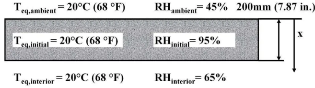
Problems that admit analytical solutions are few. Most of these problems are fairly simple involving a few materials and basic boundary conditions. One such exercise consists of modeling the moisture redistribution in a single layer of material (in this case a lightweight concrete slab under isothermal conditions). Complete details for this HAMSTAD exercise are given in Hagentoft et al. (2003) and summarized in Figure 1. The thickness of the layer was 200mm (7.87in.). The layer was initially in equilibrium with the ambient air, which has a constant relative humidity. The initial temperature was 20°C (68°F) and the initial relative humidity was 95%. Moisture transfer was caused by a sudden change in the relative humidity at the boundary conditions. The steady state exterior and interior boundary conditions were 20°C (68°F) and the relative humidities were 45% and 65% for the exterior and interior sides respectively. The structure was perfectly airtight. The case can be solved analytically. The period specified was 1000 hours.
Figure 1 – Summary of construction, initial and boundary conditions for the analytical exercise
Time step dependency
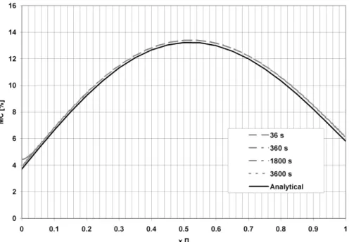
The exercise was performed using four different time steps 3600s, 1800s, 360s, and 36s. In all cases the same 51-node grid was used, 51 nodes. The moisture content in the material was independent of the
time step selected, as is shown in Figure 2, which illustrates the moisture content distribution after 1000 hours. Time step independence in this type of problem was expected, given the steady state nature of the problem. This was not the case however with all problems as will be shown in the next exercise.
Figure 2 – Moisture content profile in % through the layer at 1000 hours. The analytical solution is also included. The x-value through the layer has been normalized.
Grid dependency
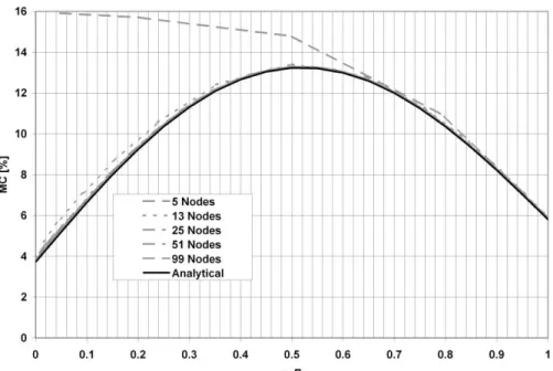
The exercise was also performed using five different grids 5, 13, 25, 51, and 99 nodes. The same time step was used for all the grid variations, specifically 3600s. Implicit solution techniques should make the solutions independent of the selection of the grid. However, the moisture content profile in the material is affected by the grid coarseness, as is shown in Figure 3. A 5-node grid did not adequately capture the correct profile. In fact, the grid size and distribution seems to exercise a considerable effect on the results. For grids with an equidistant spacing a minimum of 17 nodes is required to properly capture the phenomenon at the boundaries. For expanding grids, a minimum of 9 nodes is required to adequately capture the boundary behaviour. Overall, the first nodes should be within 5 mm of the boundaries. Recall that in this exercise the moisture transfer rates at the surfaces were high, 1·10-3 s/m (1.46·10-12 Perm-in.). This may have contribute to insatiability for solution involving sprase grids or grids where the nodes were too far from the boundaries. A 13-node grid came close to the correct profile and beyond 25 nodes there was no appreciable difference in the results. Although estimation of the total moisture content was grid independent, to obtain an adequate moisture distribution profile, a certain minimum fineness of grid was necessary. This is especially true at the surfaces where a dense grid is needed to model the heat and mass transfer processes.
Error Analysis
When an analytical solution exists, for an exercise it is possible to use statistical analysis to check the adequacy of the simulation. Two statistics are useful; the correlation coefficient, x,y, and the F-test statistic. The correlation coefficient is used to determine the relationship between two properties, in this case the predicted solution as compared with the analytical solution (Eqn. 1). The correlation coefficient is a measure of the degree of linear interrelationship between two variates. A correlation coefficient near unity indicates a strong linear relationship, though not necessarily a causal relationship.
Figure 3 – Moisture content profile in % through the layer at 1000 hours. The analytical solution is also included. The x-value through the layer has been normalized.
y x y x Y X Cov( , ) , (1) 1 1 x, y Where:
x and y are the unbiased standard deviations of both sets
)
)(
(
1
)
,
(
1y
y
x
x
n
Y
X
Cov
i n i i (2)Where: n is the sample size, and
x
andy
are the sample means.The F-test returns the one-tailed probability that the variances between two sample sets are not significantly different: i.e. whether the two samples have different variances. The F-test can be calculated through a straightforward process (Eqn. 3). The null hypothesis is that standard deviations of both sets are the same. 2 2 2 1
s
s
F
(3) Where:s
12and 2 2s
are the sample variances.The more the ratio deviates from 1, the stronger the evidence for an unequal population. Comparison of the simulation results and the analytical results are given in Table 1. The data used for the comparison was for the 13-node one-hour time-step case. The correlation coefficient, x,y, approached unity when steady state was reached, indicating a linear relationship between model and analytical solutions. The F-test values steadily improved until steady state was reached indicating that the variances (and standard deviations) of both models are similar, thus confirming the null hypothesis.
Table 1
Correlation coefficient, x,y, and F-test for the simulation and analytical solutions at 100,
300, and 1000 hours; 13 node one hour time step case. Correlation
Coefficient, x,y F-Test
Correlation
Coefficient, x,y F-Test
Correlation
Coefficient, x,y F-Test
100 hours 100 hours 300 hours 300 hours 1000 hours 1000 hours
0.999 0.926 0.999 0.936 0.999 0.994
A Common Exercise
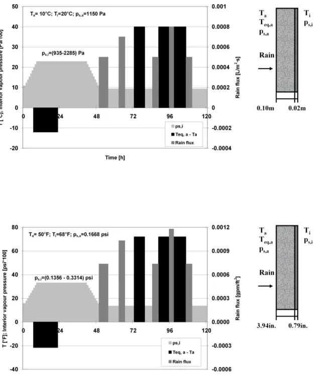
The next exercise attempted was what is called a „common exercise‟. Since most realistic situations do not admit an analytic solution, the purpose of a common exercise was to test the implementation of the physical assumptions in a model by generating a common exercise and comparing the solution of different models, an inter-program comparison. In the case of common exercises the accepted solutions can be considered to be secondary mathematical truth standards to which other programs can be compared (see ANSI/ASHRAE Standard 140 Glossary and Definitions). The exercise selected deals with moisture movement inside a wall with a hygroscopic finish. Complete details for this HAMSTAD exercise are given by Hagentoft (2003). The exterior layer is 100mm (3.94in.) thick and the finishing layer is 20mm (0.79in.) thick. The wall is subjected to changes in relative humidity as well as heat and moisture loads at the inner and outer surfaces. The boundary conditions, loads, and a schematic are summarized in Figure 4. The structure was perfectly airtight. The duration of the simulation was 120 hours. The climatic load was severe generating different heat and moisture phenomena such as condensation induced by cooling, alternating drying and wetting of the exterior layer, and moisture redistribution across the contact surface between two capillary active materials. The materials selected further complicated the case. The first layer had high values for the liquid diffusivity property thus promoting extremely fast liquid transfer. Depending on the hygrothermal tool used this exercise can be easy or difficult. In this case the tool used was a commercially available tool (designed specifically for practitioners) with limited flexibility in modifying the input parameters. The goal of the work was to conduct all exercises using the tool “right out of the box.” Cornick (2006) describes the procedure used to conduct this exercise using a practitioner‟s tool.
Error Analysis
Solutions to the above exercise “pass” if the results lie within a certain band range surrounding the “accepted” solution, considered to be a secondary mathematical truth standard. This method (i.e., use of a band of acceptance) was based on the analogy with the Student t-distribution, a statistical method for treating random data where the number of observations is low. Under such conditions, the t-distribution gives a better confidence interval than the normal distribution. The confidence interval for each calculated data point in time can be calculated from Equation 4.
n
t
x
u
n
t
x
x p x p (4)In Eqn. 4,
x
is the mean value of the sample set, x is the unbiased standard deviation of the sample set, μ is the expected value, n the number of observations, and p the total risk that the band of acceptance does not contain the true numerical solution. tp is a function of n and p. For example if the number of observations, n¸ is 8, the degrees of freedom, f, for the right tail t-distribution is 7; i.e. n-1. For the HAMSTAD benchmark exercises the confidence interval was 0.1%; i.e. a 99.9% chance that the band contains the correct solution.Grid dependency
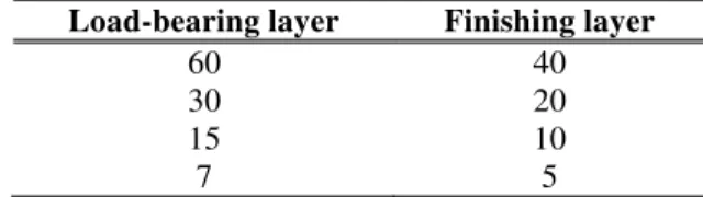
The exercise was performed using five different grids. The default grid comprised 100 nodes, 60 in the load-bearing material and 40 nodes in the finishing material. The variations are given in Table 2. The same time step was used for all the grid variations, specifically 36s. In all the grid variation exercises the result
fell within the band of acceptance demonstrating that for this exercise the solution was insensitive to the grid selection.
Time step dependency
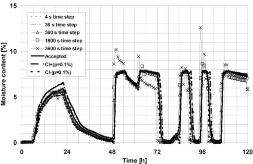
In order to investigate the effect of time steps the exercise was performed using five different time steps, 3600s, 1800s, 360s, 36s, and 4s. The same grid was used for all the time step variations, a 100-node grid. The results show that total moisture content of the load-bearing layer is dependent on the time step.
Figure 5 shows the moisture content at the outer surface. The accepted solution shown represents the average value of programs that participated in the HAMSTAD exercise (Hagentoft et al. 2003) and is considered to be the accepted solution to the exercise. The confidence limits express the band of acceptance for the 99.9% confidence grade (Cornick 2006). Longer time-steps of 1800s to 3600s generated solutions outside the band of acceptance. A time step of 360s generated results that were consistent with the HAMSTAD results and within the confidence bands. Shorter time steps produced increasingly marginal improvements if any. The same trend was apparent for the outer and inner surface temperatures, although the inner surface temperature was less affected by the exterior climate loads, and therefore the effect of changing the time step was less. Figure 6 shows the moisture content profile through the structure at 96 hours. The results were consistent, showing a pronounced effect of the time step on the results.
VALIDATION
After verifying whether the physics have been correctly implemented in a simulation tool the next step was to validate the program. Validating modeling tools consists of demonstrating that physical models implemented in the model are representative of the real world. There are two ways to validate a model. The first is to take laboratory measurements and then test the simulation against these measurements. The second is to take field measurements and test the simulation against these. In the former case controlling the boundary conditions and taking measurements is easier than in the field, however, carefully controlled laboratory experiments can be expensive and laborious. Field measurements can be as expensive or even more expensive than laboratory testing. In the field control of boundary conditions is difficult at best and the taking of appropriate measurements may be difficult if not impossible. The determinations of material properties can be difficult as well and sometime impossible depending on field-testing facilities. Both methods have advantages and disadvantages. Two examples of such exercises applied to a hygrothermal simulation tool follow.
Table 2
Grid variations for common exercise. Rows are for a particular grid. Numbers indicate the numbers of nodes per layer.
Load-bearing layer Finishing layer
60 40
30 20
15 10
Figure 4 – External and internal climatic loads (SI top and I-P bottom). Heat load from exterior is given in terms of differences between external equivalent, Teq,a, and
external air temperature Ta. Moisture load on the external side is given as a rain
flux and vapour pressure, and on the internal side as the vapour partial pressure, ps,i at a constant temperature (adapted from Hagentoft et al. 2003)
Figure 5 – Moisture content profile of the outer surface for the duration of simulation. The accepted solution is the average result of an inter-model comparison, CI+ and CI- the upper and lower 99.9% confidence limits.
Figure 6 – Moisture content profile through the structure at hour 96 of the simulation. The accepted solution is the average result of an inter-model comparison, CI+ and CI- the upper and lower 99.9% confidence limits. The x-value through the layer has been normalized.
Laboratory Testing
This exercise was based on a series of large-scale drying experiments conducted to provide benchmark data for hygrothermal models (Maref et al. 2004b; Maref et al. 2003; Maref et al. 2002a). A series of full-scale 2.43m (8ft) square samples was constructed. The basic wall, referred to as Set 1, comprised a layer of Oriented Strand Board (OSB) on the exterior side, a layer of low-density fibreglass batt insulation in a stud cavity, and a sheet of 6-mil polyethylene on the interior side. Three variations on the basic wall were also tested. The Set 2 wall was the same as the Set 1 wall except that a layer of spun bonded polyolefin (SBPO) was added to the exterior side on top of the OSB. The Set 3 wall was also the same as the Set 1 wall except that a layer of 60-minute building paper was substituted for the SBPO. The Set 4 wall was the same as Set 3 wall except that a layer of gypsum was added to the interior side on top of the polyethylene. Before testing proceeded, for each set, the OSB layer was immersed in a tank until the capillary saturation limit was nearly reached (Kumaran 1996). The constructed walls were then held in controlled climatic conditions. Drying curves for the OSB layers were determined using a precise weighing system within a climatic chamber (Maref et al. 2002b). The results of the experiments were four data sets comprising a drying curve and the concurrent environmental conditions.
Each wall set was modeled using the hygrothermal simulation tool. Materials were selected from the library of common construction materials shipped with the tool. The materials from the program library were chosen to match the materials used in the experiment where possible. The environmental chamber conditions for each set were input to the program as exterior and interior conditions as were the initial conditions. The interior surface heat transfer and moisture transfer coefficients were set to 10 W/m2·K (1.76 Btu/(h·ft2-ºF)) and 4.6·10-7 s/m (6.72·10-19 1.46 Perm-in.) respectively for the interior. Similarly the initial exterior transfer coefficients were set at 12 W/m2·K (2.11 Btu/(h·ft2-ºF)) and 5.5·10-7 (8.0·10-19 1.46 Perm-in.). Four wall simulations were run to produce predicted drying curves to compare with the observed drying curves.
Set 1: Wet OSB/Glass Fibre Insulation/6-mil Poly
. The simulation results for Set 1 showed a good correspondence with measured data. Results do show a slower predicted drying rate at the outset and a faster drying rate near the end of the test (see Figure 7). Despite this the difference between the predictions and measurements was quite small, less than 1% absolute difference (see Figure 8).Set 2: SBPO/Wet OSB/Glass Fibre Insulation/6-mil Poly
. The simulation results for Set 2 were problematic. They diverged from the laboratory data. The pattern is the same as the Set 1 results showing slower predicted drying at the outset and faster drying predicted later on. With Set 2 however the divergence near the end of the test was pronounced (see Figure 7). Error analysis suggests that there was some systematic error in the simulation, the systematic Root Means Squared Error (RMSEs) being larger than the noise in the results, RMSEu (see Figure 8). There were several possible explanations for the divergence. The material properties data of the SPBO and of OSB may have been different from those assumed. It was possible that the modeling of exterior the boundary layer of the SPBO, for example assuming perfect contact where perfect contact was not in fact obtained in the lab, was not correct or the interface between the OSB and SPBO was incorrectly modeled. After more investigation it was found that the most likely source of error was the difference between the assumed properties of the OSB and the properties of the OSB actually used. For the drying experiment the vapour permeability and suction isotherm were the most critical properties. The OSB sheathing for the experiments were selected from several batches of OSB representing different production lines and batches. The individual sheets for each of the walls were selected randomly from these batches; four sets of pairs. Other sheets of OSB were also selected randomly from the batches in order to determine the hygrothermal material properties. The data from these tests were combined with results from another project (Kumaran 2006) to form a comprehensive set. Mean values for the various material properties were determined from this set as were the upper and lower bounds (Kumaran et al. 2002). OSB is a heterogeneous material, and at the material properties were expected to vary with in certain limits even within a specific manufacturers production run. The mean values represent the material properties that were included in the stock library for the hygrothermal tool used in this study. The assumption was that the properties for any given piece of OSB would be between the upper and lower bounds. Thus, for any of the walls tested, the OSB properties may differ from thoseassumed for the simulation exercises. Sensitivity studies showed that the drying curves are sensitive to the material properties, especially the water vapour permeance property, and when compared to the drying curves generated using the upper and lower limits for the material properties for OSB, the results for Set 2 were closer to the measured results (see Figure 9).
Set 3: 60-min. paper/Glass Fibre Insulation/6-mil Poly.
Like Set 1, the simulation results for Set 3 showed good correspondence to the measured data. Initially the Set 3 results were better than the Set 1 results (see Figure 7). Halfway through the test however there was a significant difference. The moisture content of the OSB dropped and began to fluctuate. This sudden change in the response however did not seem however to be caused by any change in the conditions in the climatic chamber. The simulation tool, using the chamber data, predicted a smooth drying curve continuing from the initial phase. In this case the divergence between the modeled and laboratory results was attributed to measurement difficulties with the weighing system. The unsystematic error or noise was greater than the systematic error (see Figure 8).Set 4: 60-min. paper/Glass Fibre Insulation/6-mil Poly./Gypsum
. The simulation results for Set 4were all similar in respects to the other three. The simulations do show a slower predicted drying rate at the outset and faster drying rate near the end of the test (see Figure 7). Despite this, the error in the predictions was small (see Figure 8).
Field validation
Field validation consists of comparing computer program predictions with measurements taken in the field. Field data can be obtained from dedicated field-testing facilitates (Maref and Rousseau 2007; Straube et al. 2004; McNeil and Bassett 2007; Geving and Uvsløkk 2000) or from the monitoring of existing buildings. The measurements in the former case are considerably less difficult than the latter. In field-testing facilities there is a certain degree of control of the test parameters except the external boundary conditions. Monitoring existing buildings however presents a number of practical difficulties including but not limited to the characterization of air leakage and the determination of material properties.
In 2000 at Voll Trondheim in Norway Geving and Uvsløkk performed a field experiment on a test house. The objective was to generate experimental data for the validation of hygrothermal models. Temperature, relative humidity, and moisture content of various walls and roof sections were measured. A detailed description of the configurations and materials used for the walls and roofs as well as the experimental setup are given in Geving and Uvsløkk (2000).
The exercise considered here was based on Tariku‟s work (Tariku and Kumaran 2006). Here an east facing aerated concrete wall section 1.2m (3.94ft) wide, 0.3m (0.984ft) thick, and 3.25m (10.7ft) tall was considered. The exterior side was exposed to the ambient conditions. Conditions in the interior were 23°C (73.4°F) and 45% RH. Three temperature and relative humidity sensors were positioned at depths of 50mm (1.7in.), 150mm (5.91in.) and 260mm (10.2in.). Exterior and interior data measurements within the wall from the beginning of March 1996 through to the end of March 1998 were used. In modeling the concrete wall the concrete material properties were taken from a library of stock building materials in the program. The heat and moisture transfer coefficients for the interior were set at 8.34 W/m2-K (1.47 Btu/(h·ft2-ºF)) 5.08·10-8 s/m (7.42 10-20 Perm-in.) respectively. The initial exterior coefficients were 34 W/m2-K (5.99 Btu/(h·ft2-ºF)) and 2.07·10-7s/m (3.02·10-19 Perm-in.).
Figure 7 – Percentage error between predicted and measured total moisture contents for the OSB layers for all four walls tested.
Figure 8 – Statistical errors for all the wall sets. Mean absolute, mean bias, root mean squared error. RMSE systematic and unsystematic errors are also shown.
Drying curves for Set 2 0 0.1 0.2 0.3 0.4 0.5 0.6 0.7 0 1 2 3 4 5 6 7 8 9 10 11 12 13 14 15 16 Time [d] MC [%} OSB MC: Experimental OSB MC: hygIRC 1D 10.1 properties "+/-" 20% Vper
20% variation in vapur permeance
Average OSB properties 10.1 mm OSB properties
Experimental results
Figure 9 – Effect of changing the water vapour permeance. The average OSB properties are compared with the measured properties of a 10.1 mm sheet of OSB and a 20% variation in water vapour permeance.
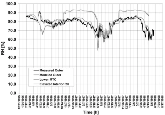
The comparison between the measured RH values and the RH predicted by the hygrothermal tool are shown in Figure 10, Figure 11, and Figure 12. Statistical measures comparing the measured and simulated responses are shown in Table 3. Though the computer predictions tracked the measured behaviour in terms of response, the program consistently over predicted the moisture content in the outer layer; the MBE was approximately 8%. Changing the moisture transfer coefficient (MTC) by an order of magnitude has a substantial effect on the results, as shown in Figure 10. The MBE was almost zero in this case and the MAE was considerably reduced as is the RMSE. However, from Figure 10, it was clear that the early events were not correctly modeled. Changing the MTC did not improve the results in the middle of the wall (see Figure 11). Not surprisingly, changing the exterior MTC had no appreciable effect on the results of the interior layer (see Figure 12). The difference in material properties may have been significant in this case. This was discussed by Tariku (Tariku and Kumaran 2006).
A significant bias was observed comparing the results at the inner layer (see Figure 12). From Table 3 the MBE was –8.6%. Tariku referred to uncertainties in the boundary conditions data suggested by Geving (Geving 1997) and speculated that a consistent underestimation of the interior relative humidity occurred. The suggested bias was 10% of measured RH, which was consistent with MBE reported in Table 3. To test this subsequent simulation runs were run using interior RH conditions 10% above the reported conditions. Raising the interior RH improved the prediction of the moisture content at the inner and middle layer (see Figure 10, Figure 11, and Figure 12) but had little effect on the moisture content near the outer layers. In general each variation on the original input improves the prediction in terms of error (see Table 3). Whether the variations can be soundly defended is not discussed here. The correlation coefficient shows some degree of correlation between the predicted and measured RH however substantial improvement could be made. Similarly the F-test suggests that variances of the data sets are substantially different and therefore the two data sets cannot be considered to be the same. Two possibilities present themselves; the simulation program did not “pass” the test or data set from the field test is flawed. No definitive determination is possible here. This case illustrates the difficulties of validating models using field test data.
Figure 10 – Comparison of measured and computed relative humidity at the outer section. Three scenarios are shown; 1) reported values and default coefficients, 2) a low MTC, and 3) an elevated indoor RH.
DISCUSSION
In this paper a commercially available hygrothermal simulation tool designed for practitioners was put through a series of exercises. No adjustments to the program were made to minimise the differences between results from simulation and those of the experiment; it was used “out of the box”. Through the use of published analytical and common exercises, it is possible to establish some confidence the in 1-dimensional hygrothermal simulation tools, and by extension other programs of similar type provided they produce similar results. This, however, is not currently possible for establishing confidence in 2- and 3-dimensional program as there are no such exercises available. Similarly there are few high quality datasets based on laboratory or field data for validating programs. The exercises presented show the difficulties encountered when trying to validate a programs. The main difficulties concern the establishment of boundary conditions, material properties, and especially the appropriate transfer coefficients. In some cases it may not be possible to adequately simulate the lab or field work especially when the input parameters are restricted, as is common in practitioner‟s tools. In the case of the program used in this paper the common exercise specified conditions could not be input. This was handled by modifying the input files to generate equivalent conditions on the surfaces. This emphasizes the point that with a good understanding of the program at hand many conditions can be successfully modeled. Material properties however are problematic. The simulation tool used in this paper allows users to define new materials. When material properties were specified it was possible to adequately complete the exercises. In cases where the material properties were not specified materials were selected from the a stock library. Lack of materials data or a constrained selection can limit a simulation tool such that a good comparsion between results may not be possible.
Another significant factor contributing to differences between laboratory experiments and simulations reported on here was the manner in which the modeling of interstitial surface boundaries was treated. Hygrothermal simulations generally assume that there is a perfect contact between layers. In fact, in real systems this is usually not the case. The net affect of this assumption is that the drying rates in the simulation runs can be decreased; i.e. increased contact resistance slows drying. This, in turn underestimates the loss in moisture content over time to the environment or other layers, and can lead to higher estimates of moisture content. Other differences can be attributed to a number of other factors such as grid size, time step, etc. For most programs that use implicit solvers, grid size and spacing are generally not an issue except at the surface boundaries. The selection of time step depends on the nature of the
problem. Problems with severe changes in boundary conditions or problems involving capillary active materials may require time steps shorter than the standard hourly time step. If a program is limited to hourly time steps, then establishing a correspondence may not be possible, as was shown in the common exercise.
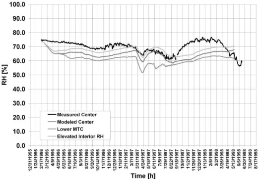
Figure 11 – Comparison of measured and computed relative humidity at the middle section. Three scenarios are shown; 1) reported values and default coefficients, 2) a low MTC, and 3) an elevated indoor RH.
Figure 12 – Comparison of measured and computed relative humidity at the inner section. Three scenarios are shown; 1) reported values and default coefficients, 2) a low MTC, and 3) an elevated indoor RH.
Statistical errors for all the wall sets; Mean absolute, mean bias, root means squared error. RMSE systematic and unsystematic errors are also given as well as the correlation
coefficient and F-Test statistic.
MAE MBE RMSE RMSEs RMSEu x,y F-Test
Case 1 2 3 1 2 3 1 2 3 1 2 3 1 2 3 1 2 3 1 2 3 Inner RH 9.1 10 5.1 -8.6 -9.5 -4.5 0.4 0.4 0.2 0.3 0.3 0.2 0.2 0.1 0.2 0.8 0.8 0.8 0.0 0.0 0.0 Inner T 0.7 0.7 0.7 -0.1 0.0 -0.1 0.1 0.1 0.1 0.0 0.0 0.0 0.1 0.1 0.1 1.0 1.0 1.0 0.3 0.3 0.3 Middle RH 6.1 9.2 4.1 -5.3 -8.6 -2.4 0.3 0.4 0.2 0.2 0.3 0.1 0.2 0.2 0.2 0.5 0.7 0.4 0.0 0.5 0.0 Middle T 0.9 0.9 0.9 -0.1 0.0 -0.1 0.1 0.1 0.1 0.0 0.0 0.0 0.1 0.1 0.1 1.0 1.0 1.0 0.3 0.2 0.2 Outer RH 8.1 3.8 8.6 7.9 -0.8 8.5 0.4 0.2 0.4 0.0 0.0 0.0 3.0 2.7 3.0 0.6 0.8 0.6 0.0 0.1 0.1 Outer T 1.7 1.6 1.7 -1.0 -0.9 -1.0 0.1 0.1 0.1 0.0 0.0 0.0 0.1 0.1 0.1 1.0 1.0 1.0 0.1 0.1 0.1
Case 1 - Reported results, 2 - Low Moisture transfer coefficient, 3 - Elevated Indoor RH; x,y - correlation coefficient
CONCLUSIONS
As with any building simulation tool, hygrothermal simulation tools used for assessing hygrothermal performance of wall assemblies should be verified and validated before users can be confident in the results. The task of validating simulation tools is evidently both a difficult and time-consuming task without appropriate tools and a methodology from which, at least, an overall assessment of the degree to which the program reproduces the measured results can rapidly be ascertained. In this paper the task of verifying and validating a hygrothermal thermal simulation tool was demonstrated using a publicly available practitioner‟s tool. The general process of the methodology followed was 1) analytical verification, 2) comparative testing, 3) and empirical validation. Analytical and comparative testing of the program was undertaken using a suite of exercises expressly validating 1-dimensional hygrothermal models. This was a comprehensive effort a portion of which was reported in this paper. The results for this particular program were very good. Similarly, empirical validation was carried out using data from laboratory and field experiments designed for such a purpose. The results here, however, were mixed.
One result that became clear was that validating hygrothermal models is difficult at best, especially without guidance. ANSI/AHSRAE Standard 140 provides the guidance for what is needed for validating building energy simulation models but there is no comparable standard for hygrothermal. First and foremost, a methodology is required. Analytical solutions should be developed where possible as well as a set of common exercises that can be used as a secondary mathematical truth standard. High quality data sets to fully exercise 1-, 2-, and 3-dimensional models are also required. Diagnostic tools also need to be developed or incorporated into the exercises analogous to the diagnostic procedures in ANSI/AHSRAE Standard 140. There have been many experiments conducted to validate laboratory simulation tools. Perhaps the results of these experiments could be collected and published as data sets to serve as benchmarks. Establishing a methodology of verification and validation of hygrothermal simulation tools is especially relevant as standards such as ASHRAE 160-2009, which give guidance for moisture design, rely on the use of hygrothermal models for compliance.
Attempting these exercises made clear another requirement for practitioners. Some form of guidance is needed to assist practitioners to make effective use of tools. Some hygrothermal models aimed at practitioners may have limited inputs, thus limiting the need for guidance. The drawback is that this limits the applicability of the tool. In this case, users can create equivalent conditions if they have a good understanding of how the tool works. If more flexibility is given, such as with the tool used here some guidance is required. Some general guidelines involving the treatment of boundaries, surface and interstitial, grid resolution, time step selection, transfer coefficients, and material properties is required. Many, but not all, of these issues have begun to be addressed in ASHRAE Standard 160-2009.
ACKNOWLEDGEMENTS
The authors are indebted to Dr. Mavinkal K. Kumaran for sharing his considerable expertise and his timely advice in the execution of this work.
REFERENCES
ASHRAE. 2007. ANSI/ASHRAE 140-2007 Standard Method of Test for the Evaluation of Building
Energy Analysis Computer Programs. American Society for Heating Refrigerating and
Air-conditioning Engineers Inc.: Atlanta, GA.
ASHRAE 2009. ASHRAE 160-2009 Criteria for Moisture Control Design Analysis in Buildings American Society for Heating Refrigerating and Air-conditioning Engineers Inc.: Atlanta, GA.
ASHRAE. 1325-RP. Environmental Weather Loads for Hygrothermal Analysis and Design of Buildings. ASHRAE Technical Committee 4.4, Building Materials and Building Envelope Performance, American Society for Heating Refrigerating and Air-conditioning Engineers Inc.: Atlanta, Ga.
http://www.ashrae.org/pressroom/detail/13535
Cornick, S. M., and W. A. Dalgliesh. 2008. Adapting rain data for hygrothermal models. Building and Environment, Vol. 44, No. 5, 2009, pp. 987-996. doi:10.1016/j.buildenv.2008.07.002.
Cornick, S. M., and M. K. Kumaran. 2008. A Comparison of empirical indoor relative humidity models with measured data. Journal of Building Physics, 31, (3), January, pp. 243-268, (NRCC-49235) URL: http://irc.nrc-cnrc.gc.ca/pubs/fulltext/nrcc49235
Cornick, S. M. 2006. Results of the HAMSTAD benchmarking exercises using hygIRC 1D Version 1.1, Research Report, Institute for Research in Construction, National Research Council Canada, 222, pp. 93, (IRC-RR-222) URL: http://irc.nrc-cnrc.gc.ca/pubs/fulltext/rr/rr222/
Cornick, S. M., R. Djebbar, and W.A. Dalgliesh. 2003. Selecting moisture reference years using a moisture index approach. Building and Environment, 38, (12), December, pp. 1367-1379, (NRCC-45674) URL:
http://irc.nrc-cnrc.gc.ca/pubs/fulltext/nrcc45674/
Geving, S., and Uvsløkk. 2000. Test house measurements for verification of heat-, air and moisture transfer models. Norwegian Building Research Report, Report no 273, Trondheim, Norway.
Geving, S. 1997. Moisture design of building constructions. Hygrothermal analysis using simulation models. Dr.ing. Thesis, Dept. of Building and Construction.
Hagentoft, C-E., O. Adan, B. Adl-Zarrabi, R. Becker, H. Brocken, J. Carmeliet, R. Djebbar, M. Funk, J. Grunewald, H. Hens, M. K. Kumaran, S. Roels, A. S. Kalagasidis, and D. Shamir. 2003. Assessment method of numerical prediction models for combined heat, air and moisture transfer in building components: Benchmarks for one-dimensional cases, pp. 26, July 22. (European Community Project HAMSTAD Technology Implementation Plan: Also published in Journal of Thermal Envelope and Building Science, v. 27, no. 4, April 2004, pp. 327-352) (NRCC-46623)
Holm Andreas, H., and H. M. Hartwig. 2002. "The influence of measurement uncertainties on the calculated hygrothermal performance." ASTM Special Technical Publication.Holm, A., and K. Lengsfield. 2007. Moisture-buffering effect experimental investigations and validation. Thermal
Performance of the Exterior Envelopes of Whole Buildings X : Proceedings of the
ASHRAE/DOE/BTECC Conference, Clearwater Beach, FL., USA, December 2-7. pp. 1-8.
Judkoff, R., J. Neymark. 2006. Model validation and testing: The methodological foundation of ASHRAE Standard 140. ASHRAE Transactions, Volume 112, Part 2, pp. 367-376. Atlanta GA: American Society of Heating, Refrigerating and Air-Conditioning Engineers.
Karagiozis, A.N., and M. H. Salonvaara. 1995. "Influence of material properties on the hygrothermal performance of a high-rise residential wall," ASHRAE Transactions, ASHRAE Symposium (Chicago, IL, USA, January, 1995), pp. 647-655, 1995 (NRCC-37913) (IRC-P-3760)
Kumaran, M.K. 2006. A Thermal and moisture property database for common building and insulation materials. ASHRAE Transactions, 112, (pt. 2), pp. 1-13, June 01, 2006 (NRCC-45692) URL:
http://irc.nrc-cnrc.gc.ca/pubs/fulltext/nrcc45692/
Kumaran, M.K., J. C. Lackey, N. Normandin, D. van Reenen, F. Tariku. 2002. Summary Report From Task 3 of MEWS Project at the Institute for Research in Construction - Hygrothermal Properties of Several Building Materials, Research Report, Institute for Research in Construction, National
Research Council Canada, 110, pp. 73, October 01, 2002 (RR-110) URL: http://irc.nrc-cnrc.gc.ca/pubs/rr/rr110/
Kumaran, M. K. 1996. Final Report Volume 3 Task 3 : Material properties. International Energy Agency Annex 24 on Heat, Air and Moisture Transport in New and Retrofitted Building Envelope Parts (Hamtie), pp. 135, International Energy Agency.
Maref, W., and M. Z. Rousseau. 2007. New field testing facility at NRC-IRC offers opportunities for wall performance assessment. Solplan Review, (135), July, pp. 18-19 (NRCC-49706)
Maref, W., S. M. Cornick, K. Abdulghani, and D. van Reenen, D. 2004a. An advanced hygrothermal design tool 1-D hygIRC Proceedings of eSim 2004 Conference, Vancouver, B.C. June 09. pp. 190-195, (NRCC-46902) URL: http://irc.nrc-cnrc.gc.ca/pubs/fulltext/nrcc46902/
Maref, W., M. A. Lacasse, and D. G. Booth. 2004b. Large-scale laboratory measurements and
benchmarking of an advanced hygrothermal model. Proceedings of CIB 2004 Conference Toronto,
Ontario, May 02. pp. 1-11, (NRCC-46784)
Maref, W., M. A. Lacasse, and D. G. Booth. 2003. An approach to validating computational models for hygrothermal analysis - full scale experiments. Proceedings of the 3rd International Conference on
Computational Heat and Mass Transfer, Banff, Alberta, May 26. pp. 243-251 (NRCC-45215) URL:
http://irc.nrc-cnrc.gc.ca/pubs/fulltext/nrcc45215/
Maref, W., M. A. Lacasse, and D. G. Booth. 2002a. Benchmarking of IRC's advanced hygrothermal model - hygIRC using mid- and large-scale experiments, Research Report, Institute for Research in
Construction, National Research Council Canada, 126, pp. 38, December 01, 2002 (RR-126) URL:
http://irc.nrc-cnrc.gc.ca/pubs/fulltext/rr/rr126/
Maref, W., D. G. Booth, M. A. Lacasse, and M. Nicholls. 2002b. Drying experiment of wood-frame wall assemblies performed in the climatic chamber EEEF: specification of equipment used in EEEF-environmental exposure envelope facility. Research Report, Institute for Research in Construction, National Research Council Canada, 105, pp. 42, (RR-105) URL: http://irc.nrc-cnrc.gc.ca/pubs/fulltext/rr/rr105/
McNeil, S., and M. Bassett. 2007. Moisture recovery rates for walls in temperature climates. Proceedings
of the 11th Canadian Building Science & Technology Conference Vol. 1, Banff Alberta, March 21-23.
pp 143-154.
Mukhopadhyaya, P., M. K. Kumaran, J. Lackey, N. Normandine, D. van Reenen, and F. Tariku. 2007. Hygrothermal Properties of Exterior Claddings, Sheathing Boards, Membranes, and Insulation Materials for Building Envelopes. Thermal Performance of the Exterior Envelopes of Whole Buildings
X : Proceedings of the ASHRAE/DOE/BTECC Conference, Clearwater Beach, FL., USA, December 2-7. pp 1-13.
Neale, A., D. Derome, B. Blocken, and J. Carmeliet. 2007a. Determination of surface convective heat transfer coefficient by CFD. Proceedings of the 11th Canadian Building Science & Technology Conference Vol. 1, Banff Alberta, March 21-23. pp 67-78.
Neale, A., D. Derome, and B. Blocken. 2007b. Coupled simulation of vapor flow between air and a porous material. Thermal Performance of the Exterior Envelopes of Whole Buildings X : Proceedings of the
ASHRAE/DOE/BTECC Conference, Clearwater Beach, FL., USA, December 2-7. pp 1-11.
Rode, C., and M. Woloszyn. 2007. Whole-building hygrothermal modeling in Annex 41. Thermal
Performance of the Exterior Envelopes of Whole Buildings X : Proceedings of the
ASHRAE/DOE/BTECC Conference, Clearwater Beach, FL., USA, December 2-7. pp. 1-15.
Salonvaara, M., Pezoulas, L., Zhang, J., and Oazera, M., “1325-RP Environmental Weather Loads for Hygrothermal Analysis and Design of Buildings,” Final Report, American Society of Heating Refrigeration and Air-Conditioning Engineers, Atlanta, GA, 2009.
Salonvaara, M., J. S. Zhang, and A. Karagiozis. 2003. Combined air, heat, moisture and VOC transport in whole buildings, Proceedings of the 7th Healthy Buildings conference (CD), Singapore, National
University of Singapore, Singapore December 7 – 12. 6 p.
Salonvaara, M., and A. Karagiozis. 1999. Whole building hygrothermal performance. Building Physics in
the Nordic Countries, Proceedings of the 5th Symposium, Göteborg, SE, Chalmers University of Technology, Göteborg, August 24 – 26. pp. 745 – 753.
Straube, J., A. Van Straaten, and E. Burnett. 2004. Field studies of ventilation drying. Proceedings of the
Performance of the Exterior Envelopes of Whole Buildings IX International Conference. Clearwater, Florida, USA. (ASHRAE 1091 Project)
Tariku, F. 2008. Whole building heat and moisture analysis, PhD Thesis, Concordia University, March 2008.
Tariku, F., S. M. Cornick, and M.A. Lacasse. 2007. Simulation of wind-driven rain penetration effects on the performance of a stucco-clad wall. Thermal Performance of the Exterior Envelopes of Whole
Buildings X : Proceedings of the ASHRAE/DOE/BTECC Conference, Clearwater Beach, FL., USA, December 2-7. pp. 1-9.
Tariku, F., and M. K. Kumaran. 2006. Hygrothermal modeling of aerated concrete wall and comparison with field experiment. Proceedings of the 3rd International Building Physics Conference, Montreal,
QC. August 27. pp. 321-328, (NRCC-45560) http://irc.nrc-cnrc.gc.ca/pubs/fulltext/nrcc45560/
Woloszyn, M., and C. Rode. 2008a. "Tools for performance simulation of heat, air and moisture conditions of whole buildings." Building Simulation 1(1): 5-24.
Woloszyn, M., and C. Rode. 2008b. IEA Annex 41: Whole Building Heat, Air and Moisture Response - MOIST-ENG: Volume 1: Modeling Principles and Common Exercises, International Energy Agency, ISBN 978-90-334-7057-8, 234 pp.