On available energy in the ocean and its application to the Barents Sea

(1)

HAL Id: hal-00298487

https://hal.archives-ouvertes.fr/hal-00298487

Submitted on 27 Nov 2007

HAL is a multi-disciplinary open access

archive for the deposit and dissemination of sci-entific research documents, whether they are pub-lished or not. The documents may come from teaching and research institutions in France or abroad, or from public or private research centers.

L’archive ouverte pluridisciplinaire HAL, est destinée au dépôt et à la diffusion de documents scientifiques de niveau recherche, publiés ou non, émanant des établissements d’enseignement et de recherche français ou étrangers, des laboratoires publics ou privés.

On available energy in the ocean and its application to

the Barents Sea

R. C. Levine, D. J. Webb

To cite this version:

R. C. Levine, D. J. Webb. On available energy in the ocean and its application to the Barents Sea. Ocean Science Discussions, European Geosciences Union, 2007, 4 (6), pp.897-931. �hal-00298487�

(2)

OSD

4, 897–931, 2007

Available energy in the Barents Sea

R. C. Levine and D. J. Webb Title Page Abstract Introduction Conclusions References Tables Figures ◭ ◮ ◭ ◮ Back Close Full Screen / Esc

Printer-friendly Version Interactive Discussion

Ocean Sci. Discuss., 4, 897–931, 2007 www.ocean-sci-discuss.net/4/897/2007/ © Author(s) 2007. This work is licensed under a Creative Commons License.

Ocean Science Discussions

Papers published in Ocean Science Discussions are under open-access review for the journal Ocean Science

On available energy in the ocean and its

application to the Barents Sea

R. C. Levine1and D. J. Webb2

1

Department of Geography, University of Sheffield, UK 2

National Oceanography Centre, Southampton, UK

Received: 12 November 2007 – Accepted: 12 November 2007 – Published: 27 November 2007

(3)

OSD

4, 897–931, 2007

EGU Abstract

Following meteorological practice the definition of available potential energy in the ocean is conventionally defined in terms of the properties of the global ocean. However there is also a requirement for a localised definition, for example the energy released when shelf water cascades down a continental shelf in the Arctic and enters a boundary

5

current.

In this note we start from first principals to obtain an exact expression for the avail-able energy (AE ) in such a situation. We show that the availavail-able energy depends on enstrophy and gravity. We also show that it is exactly equal to the work done by the pressure gradient and by buoyancy.

10

The results are used to investigate the distribution of AE in the Barents Sea and surrounding regions relative to the interior of the Arctic Ocean. We find that water en-tering the Barents Sea from the Atlantic already has a highAE , that it is increased by cooling but that much of the increase is lost overcoming turbulence during the passage through the region to the Arctic Ocean. However on entering the Arctic enough

avail-15

able energy remains to drive a significant current around the margin of the ocean. The core of raised available energy also acts as a tracer which can be followed along the continental slope beyond the dateline.

1 Introduction

RecentlyLevine(2005) investigated the dynamic height or pressure field of the Arctic

20

Ocean making use of results from the OCCAM global ocean model (Webb et al.,1998). He found that along the boundary of the Arctic, at depths of a few hundred metres, the largest dynamic heights occur where dense Barents Sea shelf water cascades down the continental slope in the St Anna Trough. This water becomes part of a bound-ary current whose waters can be followed eastwards around the Arctic and out in the

25

(4)

OSD

4, 897–931, 2007

This result raises a number of questions concerning the energetics of the flow. Boundary currents need energy to start the current and to overcome boundary tur-bulence. So how much of the energy available to the current comes from the release of potential energy as the water descends the St Anna Trough? What effects do the density changes due to cooling and ice formation in the Barents Sea have on the

pro-5

cess? How much of the energy is implicit in the water flowing into the Barents Sea from the Atlantic? We also need to know how changes in internal energy and, in analogy to Bernouilli’s equation, the large scale oceanic pressure field may also be involved.

If we concentrate first on gravitational potential energy, previous studies of the ocean have been based on the atmospheric definition of Available Potential Energy (AP E ).

10

Lorenz (1955) defined this to be the difference between the Potential Energy (P E) of the atmosphere under study and the P E of a reference atmosphere produced by moving the air parcels adiabatically (i.e. reversibly) so that the atmosphere reaches its minimumP E state. Thus,

AP E = Z V₁gρz d V − Z V₂ gρrz d V, (1) 15

whereρ is the density, ρr the density of the reference system, z is height, and the

integrals are over the volume of the original systemV1, and the reference systemV2. However for our study we are more interested in the energy available to the current while it is in the Arctic. Thus we need the potential energy relative to the offshore Arctic Ocean. We also should include changes in internal energy. For a perfect gas,

20

the global change of internal energy is proportional to theAP E (Wells,1997), a result which is often sufficient for atmospheric studies. For the ocean, with its more complex equation of state, we need to be more specific.

Finally we need to include the effects of pressure. A boundary current is usually driven by pressure differences along the current, the energy for the process ultimately

25

coming from changes in potential or internal energy elsewhere in the system. If the energy for the Arctic boundary current comes ultimately from outside the region then the large scale pressure field should contain this information.

(5)

OSD

4, 897–931, 2007

EGU

To make some sense of this we start from some fairly basic thermodynamics and investigate the energy released when a parcel of water is transferred from one region of ocean, at a depthz1and pressureP1, to a second region of ocean, at depthz2and pressureP2. As energy is a conserved quantity, this equals the total energy released when the parcel is extracted for the ocean at pressureP1, moved vertically from z1 to

5

z2and injected back into the ocean at pressureP2.

We show that if the parcel of water stays within the ocean, then this equals the energy change due to the horizontal pressure gradient and vertical buoyancy forces, the total being independent of the path chosen. The result thus includes the contribution of gravity and pressure but we show that it also includes the contribution of any change

10

in internal energy. The form of the equation also allows us to split the total energy available, at each point in the fluid, into its gravitational and pressure components.

In writing this paper we have had a problem in the correct description of the energy available to drive a current. The terms potential energy or relative potential energy are obviously wrong because they leave out the contribution of pressure and internal

15

energy. Relative enthalpy has a similar problem. It includes the internal energy and pressure components but leaves out gravity. We therefor use the term available en-ergy (AE ) with the understanding that a more apt description is always welcome (see Appendix 2).

As an example of how the concept may be used, we investigate the distribution of

20

AE in the water masses passing through the Barents Sea into the Arctic Ocean. We find that the inflowing Atlantic water has a large AE compared to the central Arctic, that theAE increases as the water flows through the Barents Sea, but that much of the increase is later lost overcoming turbulence. However on entering the Arctic Ocean enoughAE remains to drive a significant current around the margin of the ocean. The

25

core of raised available energy also acts as a tracer which can be followed far along the continental slope.

(6)

OSD

4, 897–931, 2007

Printer-friendly Version Interactive Discussion 2 Internal energy and enthalpy

As shown in many textbooks (Pippard,1961), the internal energy ∆U of a mass of fluid may be changed by the addition or removal of heatQ or mechanical energy W ,

∆U = Q + W (2)

By convention such quantities are defined per unit mass of fluid. If a change is carried

5

out adiabatically, then there is no heating or cooling andQ is zero. If in addition the only mechanical energy change is due to compression thenW is equal to −P dV , where P is the pressure and d V is the change in volume. Thus for adiabatic changes in the ocean,

d U = −P dV (3)

10

To calculate the available energy of a small parcel of water, we first consider how much energy is required to move it into position from a reservoir at the same depth using a piston. If the fluid in a reservoir is at pressureP_r and the ocean at pressureP1then the work required to do thisW1is given by,

W1= − ZV₁

Vr

P d V + P1V1− PrVr, (4)

15

whereV_r and V1 are the volume per unit mass before and after injection. Physically, the first term on the r.h.s is the change in internal energy, the work expended by the piston during the initial compression phase when the pressure increases fromPr toP1 and the volume decreases fromV_r toV1. The term P1V1 is the work expended by the piston pushing fluid into the ocean at pressureP1and the last term is the help given to

20

the piston by the pressure from the reservoir as the fluid is injected1.

1

Pumping up a bicycle tyre is similar with an initial compression stage followed by an (ap-proximately) constant pressure injection stage.

(7)

OSD

4, 897–931, 2007

EGU

If the injection occurs at the bottom of the ocean, then the term P1V1 is also the energy required to raise the column of water above the point of injection to make way for the injected water. This is because the pressure equals the weight of the column of water, P1= g Zz₀ z₁ ρ(z)d z. (5) 5

wherez0is the ocean surface. So, if the column has unit area, it is raised by a distance V₁. Thus,

P1V1= Zz₁

z₀

(gρ(z)V1)d z, (6)

is the total change in potential energy of the column. If the injection is above the ocean bed, the injected water compresses the deeper water slightly, so some of the energy

10

goes into extra internal energy of the deeper water.

A more compact form of the energy involved can be obtained in terms of the thermo-dynamic quantity enthalpyH. This is defined as,

H = U + P V. (7)

Using this, Eq. (4) simplifies to become,

15

W1= H1− Hr, (8)

whereH_r andH1are the enthalpies of the fluid before and after injection.

If the reservoir and injection points are at different depths, then there is also a change in gravitational potential energy. The total energy change, the available energy, is thus,

AE = (H1+ g z1) − (Hr+ g zr). (9)

20

(8)

OSD

4, 897–931, 2007

The result is related to Bernoulli’s equation for a fluid in a gravitational field. If the two points are joined by a streamline and if the flow is both inviscid and adiabatic, then the available energy equals the change in kinetic energy per unit mass (Landau and

Lifshitz,1959) along the streamline. If the fluid is also incompressible,V is a constant, so_{H equals P/ρ and AE equals the change of (P/ρ+gz). The latter is often called the}

5

Montgomery potential.

For the problem considered later in this paper, the points may not be linked by steam-lines, the flow may not be adiabatic and much of the energy may be lost in turbulence. However the concept of available energy is still useful because of the insight it provides into the energy potentially available at each point in the flow.

10

3 Available energy as a path integral

The expression forAE (Eq.9) depends on scalar quantitiesH and z, both of which are continuous throughout the ocean. As a result the equation can be rewritten as a path integral between the initial and final pointsS1andS2. Thus,

AE = ZS₂ S₁ d s · (∇H + g ˆz). (10) 15 From Eq. (7), ∇H = ∇U + ∇(P V ) = −P ∇V + ∇(P V ) = V ∇P (11)

The volume per unit mass (V ) is the inverse of the density ρ, so, AE =

ZS2

S₁ d s · V (∇P + gρ ˆz),

(9)

OSD

4, 897–931, 2007

EGU

the first term on the r.h.s including both the effects of the pressure gradient and any change in internal energy. If the ocean is in hydrostatic balance,

AE = ZS₂

S₁ d s · V (∇hP + g(ρ − ρ0

) ˆz), (13)

where ∇hdenotes the horizontal version of the gradient operator andρ0is the ambient density field. At each point along the path, the force per unit volume acting on the

5

parcel of water is,

F = ∇hP + g(ρ − ρ0) ˆz, (14)

the second term corresponding to Archimedes’ Principle.

For analysing the available energy of shelf waters relative to the neighbouring ocean it is convenient to split the path integral of Eq. (13) into a horizontal section, in which

10

the water is first moved horizontally without change in depth, and a vertical section, in which energy is released as the partical moves vertically, within a reference water column, to a final depth where it has the same density as the surrounding water mass. Thus, AE = AEp+ AEg, (15) 15 where, AE_p= ZS₂′ S1 d s · V ∇hP, (16) = ZP₂ P₁ d P V, (17)

is the contribution from the constant depth section and AE_g =

Zz2

z1

d z V g(ρ − ρ0), (18)

(10)

OSD

4, 897–931, 2007

is the contribution from the final vertical section. Herez1andz2are the initial and final depths andP1andP2are the pressures at pointsS1andS2′, the latter being at the final geographical position but at the initial depth. In the rest of this paper we refer toAE_p andAE_g as the pressure and gravitational contributions to the Available Energy.

AsV equals 1/ρ, and ρ is almost constant within the ocean,

5 AE_p≈ (P1− P2)/ρ′_, ₍₁₉₎ AE_g ≈ (1/ρ′) Zz2 z₁ d z g(ρ − ρ0 ), (20)

whereρ′ is a typical density in the region. The approximation is similar to that used in Eq. (1), in that it ignores the changing internal energy due to changes in pressure. The

10

size of the error introduced depends on the range of densities involved but will usually be of order 1% of the total or less.

IfAE_p′ andAE_g′ represent the corresponding values per unit volume, then to the same approximation, AE_p′ ≈ (P1− P2), (21) 15 AE_g′ ≈ Zz₂ z1 d z g(ρ − ρ0). (22)

4 Available energy in the Barents Sea

As an example of how these concepts may be used, we consider the results from a model study of the flow through the Barents Sea towards the St. Anna Trough. The

20

data that we use comes from a run of the 1/12◦ version of the OCCAM global ocean model (Webb et al.,1998;Coward and de Cuevas,2005).

(11)

OSD

4, 897–931, 2007

EGU

The model is forced by NCAR surface fluxes and the run presently covers the period 1985 to 2004. Time series from the Barents Sea region of the model show year to year variability but no long term drift. The model Barents Sea is well mixed in the vertical at the end of winter and becomes stratified during the summer months with a warmer and fresher surface layer. For the results presented here we used the monthly averaged

5

model data from February 1998. 4.1 The Barents Sea water masses

The Barents Sea (Fig. 1) is a relatively deep region of continental shelf, with large areas below 200 m. The main central region is connected to the Norwegian Sea in the west via a deep trough, the Bear Island Trough, with depths below 400 m. In the

north-10

east there is an even deeper trough, the St Anna Trough, with depths below 500 m connecting the region to the Arctic Ocean. The velocity field from the model shows a significant flow between the two troughs, the main restriction to the flow appearing to be a narrow sill near 57.5◦E 78◦N, with a depth of approximately 200 m.

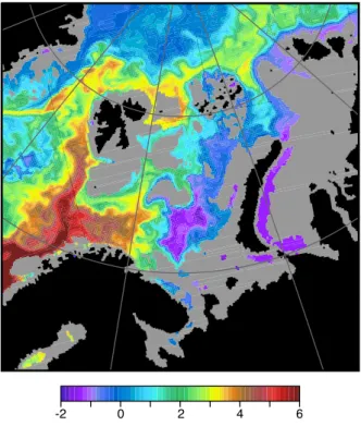
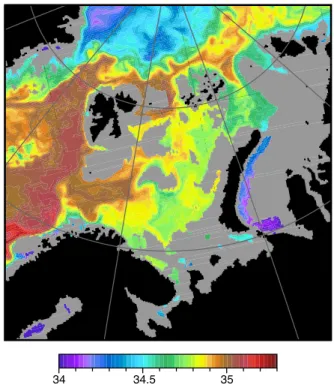
Figures 2 and 3 show the mean temperature and salinity on model level 21 in

Febru-15

ary 1998. This model level has a central depth of 205 m and a thickness of 20 m and so includes the lowest water mass passing through the sill. In the south-west, warm (> 5◦C) water enters the Barents Sea along the southern edge of the trough. Offshore this is saline (>34.9) Atlantic Water but there is also a fresher coastal current with salinities below 34.5. This water is cooled and freshened in the Barents Sea, part then

20

returns west to join the West Spitzbergen Current and part flows northwards, eventually entering the Arctic near 45◦E.

The remainder continues east, where at the end of winter it forms a large water mass in the Central Basin (45◦E, 75◦N) with temperatures near freezing (−1.9◦C) and salinities near 34.8. The flow continues north-east via the sill, mixing with other water

25

masses including cold fresh Kara Sea water, until it reaches the St Anna Trough where it sinks down the continental slope into the Arctic.

(12)

OSD

4, 897–931, 2007

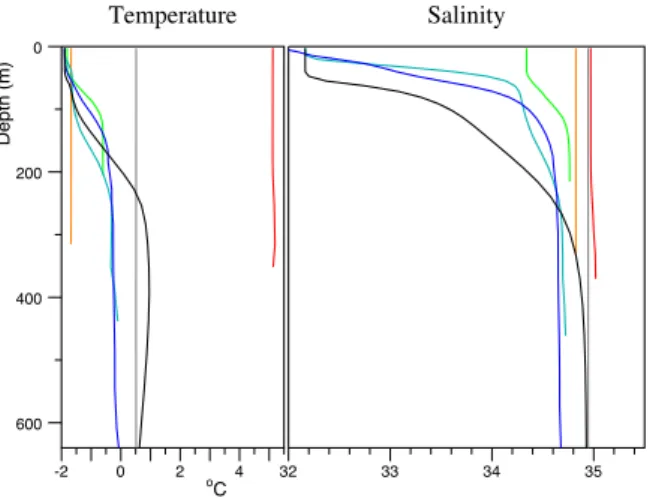
marked in Fig. 1, are shown in Fig.4. In the western and central Barents Sea, illus-trated by profilesA and B, stratification is weak or non-existant. The temperatures and salinities shown in Figs. 2 and 3 for this region are thus representative of the whole water column. Further east and north, in the St Anna Trough and the offshore Arctic Ocean (profilesC and D), a fresh surface mixed layer is found with salinities below 33

5

in the offshore Arctic. Here the mixed layer is around 100m deep and the surface fresh-ening extends down to almost 400 m. In the St Anna Trough the depth and amount of freshening is reduced, but further east in the Kara Sea the near surface salinities are again below 33. The hydrography and flows in the region are discussed further by Aksenov et al. (2007)2.

10

4.2 Density profiles

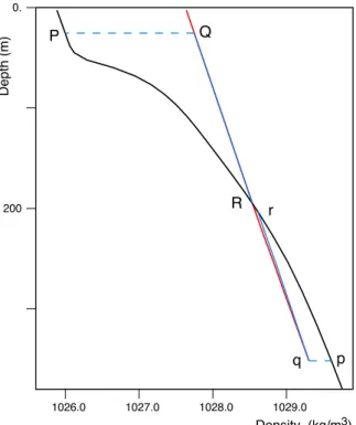
The density profiles for the seven representative stations are shown in Figs.5 and 6. In Fig.5, the profiles for the Barents Sea inflow (red) and the Arctic reference region (black) are plotted together with two adiabatic curves (blue). These show how the Barents Sea near surface (or bottom) water changes density as it sinks (or rises) to a

15

depth where it is in equilibrium with the offshore water mass.

The near surface water, point Q, is denser than that of the Arctic, P , so it has the potential to sink down the Arctic continental slope, to R, releasing energy. The total amount of gravitational energy released is approximately proportional to the area P-Q-R. (Eq. 20). Although the offshore is represented here by a single point, G, the

20

comparisons and results are similar if one uses an area average of the offshore Arctic. Deeper in the water column, the water entering the Barents Sea is lighter than that at the same depth in the offshore Arctic. As a result it can release gravitational energy by rising up in the water column. For the bottom water at pointq in Fig.5, the amount of energy released is given approximately by the area p-q-r. Water at other depths

25

2

Aksenov, Y., Bacon, S., and Coward, A.: The North Atlantic Inflow into the Nordic Seas and Arctic Ocean:A High-resolution Model Study, Deep-Sea Res. Part I, submitted, 2007.

(13)

OSD

4, 897–931, 2007

EGU

of profile A would also tend to settle out near 180 m, so that if it could easily enter the Arctic the whole water column should generate a layer or boundary current at this depth.

The density profiles of Fig.6can be interpreted in a similar manner. In the central Barents Sea, locationB, the whole water column is well mixed so the adiabatic profiles,

5

if plotted, would overlie the actual density profile. The cooling has also increased the density, but although the change is small, the equilibrium depth in the Arctic has increased from 180 m to nearer 1000 m. Thus it now has the potential of forming one of the deepest layers of the Arctic Ocean.

As this water masses passes the sill connecting the region with the St Anna Trough,

10

it mixes with cold fresher water from the Kara Sea and with warm saline Atlantic Wa-ter which has followed the longer path north of Spitzbergen. As a result the deeper water in the St Anna Trough may still release energy by sinking into the Arctic, but the equilibrium depth is reduced to 300 m.

4.3 Components of available energy

15

For analysis of available energy in the Barents Sea we make use of Eqs. (19) and (20). The range of depths involved is only a few hundred metres so the errors from ignoring the density changes due to pressure will be less than 1%.

We need to define a region that is “representative” of the offshore Arctic Ocean. For the results presented in this section we used a region roughly 100 km by 100 km

20

surrounding pointG. Calculations which used a single vertical column at point G as the representative region gave similar results.

In terms of the model variables, the component ofAE due to the pressure difference, Eq. (19), is

AE_p′(x, zn) = (P (x, zn) − P0(zn))/ρ′. (23)

25

(14)

OSD

4, 897–931, 2007

Printer-friendly Version Interactive Discussion + n−1 X i =1 (d z_iρ(x, z_i) + dz_{i +1}ρ(x, z_{i +1})))/2, (24)

whereP (x, zn) is the pressure at positionx and model level n, AP is the atmospheric

pressure,SSH the sea surface height, g gravity, d z_i the thickness of model leveli and ρ the density. P0(zn) is the average pressure at leveln in the offshore reference region.

The component due to gravity is

5 AE′ g(x, zn) = (g/ρ′)( m X i =n abs((ρ(x, z_i) − ρ0(z_i))d z_i) −((ρ(x, zn) − ρ0(zn))d zn +(ρ(x, zm) − ρ0(zm))d zm)/2), (25)

whereρ0(z) is the density in the offshore region and zm the level at which the initial

water mass reaches the same density as the offshore water.

10

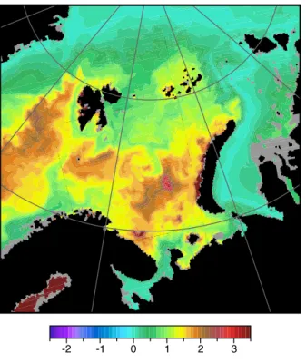
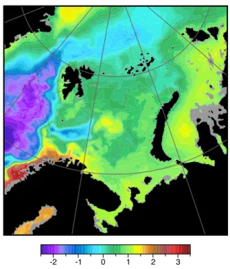
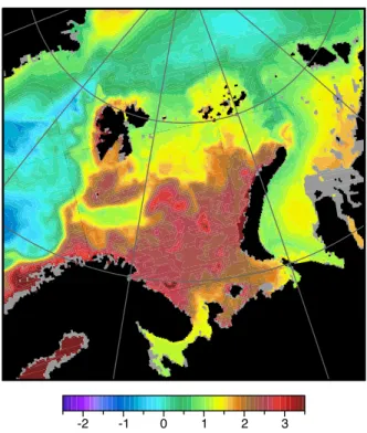
Vertical profiles of these quantities and their sum are shown in Fig.7, for the water columns discussed previously. Horizontal plots are presented in Figs. 8 to 13, for depths of 25.5 m and 205 m. These correspond to levels 5 and 21 of the model.

We have taken point A to be representative of the water masses entering the Barents Sea. The point lies on the south side of the deep trough where a current enters the

15

Barents Sea region. It also lies just outside the narrow region of high near surface pressures found along the Norwegian Coast (Fig.9). Inflow is also found in this region but dynamically it appears to be more complicated. For example the higher pressures, due to high sea level, drop off rapidly towards 30◦E, possibly due to mixing. This is discussed further below.

20

Near the surface (Fig.8), the gravitational component ofAE is generally low through-out the inflow region. Further sthrough-outh in the Norwegian Coastal Current, values ofAE range from 1.1 J/kg in the surface fresh water near the coast to 1.7 J/kg on the central

(15)

OSD

4, 897–931, 2007

EGU

Norwegian Sea side of the current1. Most of the inflow to the Barents Sea comes from the coastal side of the current but the value of 1.53 J/kg as found at point A, although slightly high, is not unreasonable.

4.4 Vertical profile of AE

The profile of AE for point A (Fig. 7) shows that, near the surface, the gravitational

5

component dominates. It drops off rapidly with depth, a result of the rapid reduction in the area integral of Fig. 5, and becomes zero near 180 m, where the density of the water in the main column equals that in the reference region. The gravitational component then increases nearer the bottom.

In contrast the pressure component has a minimum at the surface and increases with

10

depth, reaching a maximum at 180 m. Like the reduction in the gravitational term, the increase arises because the water at these depths is denser than that in the reference region. Lower in the water column the pressure difference is steadily reduced.

An important consequence of this behaviour is that the totalAE is almost constant throughout the water column. This is because the column is well mixed and because

15

the totalAE is independent of the path of integration. If AE (z1) and AE (z2) are the values ofAE at two depths in the same water column, then from Eq. (13),

AE (z1) − AE(z2) = Zz2

z1

d z V g(ρ(z) − ρ1(z)). (26)

whereρ1(z) is the density of the water column at depth z and, as before, ρ(z) is the density of the water atz1 when moved adiabatically to z. If the water is well mixed

20

between two depths, then the value of the integral is zero over the range and the available energy is constant.

1

If fully converted to kinetic energy, anAE of 1 J/kg generates a current of approximately

(16)

OSD

4, 897–931, 2007

4.5 The central Barents Sea

Reference point B lies near the centre of the dense water region. At the surface the gravitational component ofAE increases to near 3.2 J/kg, over twice its initial value, due to the water getting colder and denser. The pressure component decreases slightly but their sum increases from 1.8 J/kg at station A to 3.0 J/kg at B.

5

Deeper in the water column, the gravitational component (Fig.11) drops to around 0.5 J/kg and the pressure term (Fig.12) increases such that the total remains almost constant. What is also interesting here is that the pressure term is similar to that found near 20◦E, along the northern coast of Norway. However there it is due to high sea level whereas at pointB, where sea level is lower, it is due to high densities in the water

10

column.

4.6 St. Anna Trough

Figure 13 shows that the main exit route for the high AE water mass is through the narrow sill region at 58◦E, 77.5◦N, into the St. Anna Trough. The totalAE has values of around 2.5 J/kg at the entrance to the sill. After passing the sill, the value has

15

dropped to around 2.1 J/kg. The flow then forms a narrow boundary current along the southern and eastern boundaries of the trough. At the same time the available energy continues dropping, to values near 1.8 J/kg on the eastern side and to 1.6 J/kg at the exit of the trough. The vertical profile ofAE remains almost constant near the bottom, so although the current tends to descend in the St Anna Trough, the values of AE

20

shown in Figs.8to13are similar to the near bottom values.

Comparison of Figs. 11,12 and 13, shows that the change inAE across the sill is primarily due to the change in pressure. There is a slight increase in kinetic energy, the current increases from 10 cm s−1 to 26 cm s−1, but in the model the pressure drop is balanced primarily by the bottom friction term in the lowest model layer. ThusAE is

25

being lost overcoming the resistance due to turbulence near the sea bed.

(17)

OSD

4, 897–931, 2007

EGU

depth is around 200 m, the bottom model level has a thickness of from 5 to 20 m. Above the bottom, viscous and inertial effects are small, so there is only a slight pressure drop along streamlines. However in the south of the trough, the flow follows topography and so it is strongly affected by bottom friction along most of the path. On the eastern side of the trough the current moves into deeper water and there is less decline in totalAE .

5

4.7 The Arctic Ocean

At the exit of the St Anna Trough the water mass extends down to 350 m, with values of AE above 1.4 J/kg. This then forms a band of high AE which can be followed eastwards along the edge of the Siberian Shelf. The model water shows some dense water entering the Arctic from a second trough, the Voronin Trough near 28◦E, but

10

St Anna Trough outflow appears to the dominant water mass involved. Waters with similarAE also enter at this depth directly from the Norwegian Sea, passing north of Spitzbergen, but by the time they reach the St Anna Trough theirAE has dropped to below 1.2 J/kg.

As an example, Fig. 14 shows profiles of AE along two sections. Both are roughly

15

at right angles to the continental slope, the first near 155◦E, the second near 180◦W. Water mass withAE greater than 1.3 J/kg shows up clearly in both sections adjacent to the continental slope. High values ofAE are also found further east as far as the Alaskan continental slope but in this region the separation from the surface layer is less clearly defined.

20

Profiles of potential temperature and salinity, on the sections of Fig. 14, show a slight dipping of the constant temperature and salinity surfaces near the slope, but they provide no comparable signature to the St Anna Trough waters. It may be possible to use a combinedT/S property as a tracer but the present results indicate that, in numerical models at least,AE is a useful independent property that can be used in this

25

(18)

OSD

4, 897–931, 2007

Printer-friendly Version Interactive Discussion 5 Summary and discussion

This paper has introduced a local version of available energy to quantify the energy available relative to some nearby large body of water. This energy, which is available to accelerate currents and overcome friction, results from the changes in both enthalpy and gravitational potential energy that could occur if the water was to move from its

5

initial position to a position of equilibrium in the reference water column.

We have shown that the available energy can also be expressed as a path integral and that the integral involves two terms. The first depends primarily on the horizontal pressure gradient and the second on the vertical buoyancy force.

5.1 The Barents Sea

10

We have used these results to investigate the energetics of the Barents Sea in a high resolution ocean model. The model shows that the Atlantic inflow in the Norwegian Sea does have significant available energy relatively to the Arctic Ocean, but that this is significantly increased by cooling in the Barents Sea. The cooling also significantly increases the depth at which the Barents Sea water would settle in the Arctic Ocean.

15

The model also shows that much of the increased available energy is lost to bottom turbulence as the water crosses the Barents Sea and enters the St Anna Trough. How-ever sufficient energy remains for the outflowing St Anna Trough water to be traced far along the continental slope. This means that available energy may be a useful tracer quantity for such flows.

20

5.2 Wider impact

The results emphasise that even without the Barents Sea, the Alantic inflow has signif-icant available energy relative to the Arctic. As a result it is surprising that there isn’t a greater exchange flow through Fram Strait.

Figures9and12show that there is a significant pressure drop at the strait,

(19)

OSD

4, 897–931, 2007

EGU

phy steering much of the Spitzbergen Current into the East Greenland Current. The small throughflow may therefore be due to the limited width of Fram Strait and to the weak stratification, both of which can limit the strength of baroclinic instabilities which could mix the Atlantic water northwards. Weak stratification, together with the rough topography of the region, may also produce topographic blocking of any throughflow.

5

Given the importance of geostrophy it is noticeable that the only water continuing northwards tends to be in the boundary currents, adjacent to continental slope and the ridge offshore, where frictional effects due to turbulence allow the current to cross pres-sure contours. The importance of turbulence, in allowing ocean currents to overcome geostrophy and cross pressure contours, is often overlooked. However it is important

10

in western boundary currents and appears to be important in Fram Strait.

The present work also highlights a similar role for turbulence in the Barents Sea where it impedes the flow but also allows the flow to cross pressure contours into the Arctic Ocean. If there were no turbulence, the flow would be geostrophic and presumably there could then be no flow via the Barents Sea into the Arctic.

15

So turbulence in the Barents Sea may be increasing the flow of Atlantic Water into the Arctic. Further work is needed, for example to check that the Barents Sea trans-port does not indirectly reduce the Fram Strait transtrans-port through some other process. However even if it does, as shown byLevine(2005), the St Anna Trough outflow still has a significant impact on a flow which reaches around the Arctic and Atlantic Oceans

20

as far as Cape Hatteras.

Appendix A

Total available energy

In analogy with Eq. (1), we define the total available energy (AEtot) to be the integral of

25

AE relative to an ocean in which it is in its minimum state. Assume that the water is initially in a reservoir where both the pressureP_r and height z_r are zero. We split the

(20)

OSD

4, 897–931, 2007

ocean into columns of water and fill each column from the bottom. IfU_r is the internal energy of the water in the reservoir, then from Eq. (9) the energy required is

AE = Z dx d y Zzb z_t d z ρ(H1− Ur+ gz1) (A1)

wherex and y are the horizontal coordinates and z the vertical co-ordinate. H1,Ur and

ρ are functions of all three coordinates and the ocean bottom, z_b, is a function ofx and

5

y only. Substituting for H1and replacingdxd yd z by the volume integral d V , AE =

Z

d V ρ(U1− Ur+ P1V1+ gzb). (A2)

Substituting forP1from5and rearranging, AE = Z d V ρ (U1− Ur+ g z). (A3) Thus, 10 AEtot = Z V₁ d V ρ (U1+ g z) − Z V₀ d V ρ (U1+ gz). (A4)

where the second integral is over the minimumP E ocean and the Ur terms for the two

oceans have cancelled.

As expected the result is equal to the gravitational APE (Eq.1) plus the difference in the internal energies of the initial and minimumAE oceans. The latter arises from the

15

different pressure distributions in the two oceans (Eq.3).

Appendix B Terminology

The origin of the concept of enthalpy appears to be in dispute, but Heike

Kamerlingh-20

(21)

OSD

4, 897–931, 2007

EGU

originally defined the enthalpy functionH,

H = E + P V, (B1)

whereE is the total energy of the system including the contribution of any external field such as the gravitational potential. If this were still in use then Eq. (9) would describe relative enthalpy. Unfortunately enthalpy as commonly used now (Eq.7) includes only

5

the internal energy.

Other possibilities besides “available energy” are the terms “relative total enthalpy” and “relative gravitational enthalpy”. Note the term “gravitational enthalpy” is also used in describing hydrodynamical equilibrium in the theory of pulsars (Chubarian et al.,

2007).

10

Acknowledgements. We wish to thank to A. C. Coward, B. A. De Cuevas and Y. Aksenov for

their work in developing and running the OCCAM model and for their help with the present analysis of the archived model data.

References

Chubarian, E., Grigorian, H., Poghosyan, G., and Blaschke, D.: Deconfinement transition in

15

rotating compact stars,http://arxiv.org/abs/astro-ph/9903489v3, 2007.916

Coward, A. and de Cuevas, B.: The OCCAM 66 level model: model description, physics, initial conditions and external forcing, Tech. rep., Southampton Oceanography Centre, Internal Document No. 99, 83 pp., 2005.905

Landau, L. and Lifshitz, E.: Fluid mechanics, Pergamon Press, 536 pp., 1959.903

20

Levine, R.: Changes in shelf waters due to air-sea fluxes and their influence on the Arctic Ocean circulation as simulated in the OCCAM global ocean model, Ph.D. thesis, Graduate School of the Southampton Oceanography Centre, University of Southampton, 255 pp., 2005. 898,

914

Lorenz, E.: Available potential energy and the maintenance of the general circulation, Tellus, 7,

25

157–167, 1955. 899

Pippard, A.: Elements of Classical Thermodynamics, Cambridge University Press, 165 pp., 1961. 901

(22)

OSD

4, 897–931, 2007

Webb, D., de Cuevas, B., and Coward, A.: The first main run of the OCCAM global ocean model, Tech. Rep. 34, Southampton Oceanography Centre, 44 pp., 1998. 898,905

Wells, N.: The Atmosphere and Ocean: A Physical Introduction, John Wiley & Sons, New York, 347 pp., 1997. 899

(23)

OSD

4, 897–931, 2007

Printer-friendly Version Interactive Discussion EGU D A _B C E F G 100 0 1000 6000 70º N 30º E 60º E 90º E 0º E 80º N

Fig. 1. Bathymetry of the Barents Sea and surrounding regions, showing the depth in metres. The points markedA to G are the positions of the profiles of Figs.4 to7. A – Inflow current; B – Central Basin; C – Sill region; D – St Anna Trough; E – Arctic Boundary Current; F –

(24)

OSD

4, 897–931, 2007

0 2 4 6

-2

(25)

OSD

4, 897–931, 2007

EGU

34.5 35

34

(26)

OSD

4, 897–931, 2007

Printer-friendly Version Interactive Discussion -2 0 2 4 600 400 200 0 o C D e p th (m) Temperature 32 33 34 35 Salinity

Fig. 4. Potential temperature and salinity profiles at the seven locations of fig.1. Location:A –

(27)

OSD

4, 897–931, 2007

Printer-friendly Version Interactive Discussion EGU 1026.0 1027.0 1028.0 1029.0 200 0. Density (kg/m3) D e p th (m) Density P Q R _r q p

Fig. 5. Density profiles for locationA (red), at the Atlantic entrance to the Barents Sea, and for

the reference locationG (black) in the offshore Arctic. Using Eq. (20), the gravitational part of the available energy at depthA, relative to the offshore water column, is proportional to the area

of the region P-Q-R. The upper blue line Q-R shows the change in the density of the water as it sinks adiabatically to its equilibrium depth offshore. The lower blue line q-r shows the density change as the bottom water on the shelf rises to its equilibrium depth offshore.

(28)

OSD

4, 897–931, 2007

Printer-friendly Version Interactive Discussion 1026.0 1027.0 1028.0 1029.0 1030.0 1031.0 600 400 200 0 Density (kg/m3₎ D e p th (m)

Fig. 6. Density profiles for locationsA to G of Fig.1. Location: A – red – Barents Sea inflow; B – brown – Central Basin; C – green – Sill region; D – blue-green – St Anna Trough; E – blue

– Arctic Boundary Current; F – grey – Norwegian Sea; G – black – Arctic Ocean reference

(29)

OSD

4, 897–931, 2007

Printer-friendly Version Interactive Discussion EGU 600 400 200 0 D e p th (m) AE 0 1 2 3 J/_kg 600 400 200 0 D e p th (m) 0 1 2 3 J/_kg 0 1 2 3 J/_kg

(a) Barents Sea Inflow

(b) Central Basin (c) Sill region

(d) St Anna Trough (e) Arctic Boundary Current (f) Norwegian Sea

Fig. 7. Gravitational (red), pressure (green) and total (blue) components of available energy at locationsA to F of Fig.1relative to locationG.

(30)

OSD

4, 897–931, 2007

0 1 2 3

-2 -1

(31)

OSD

4, 897–931, 2007

EGU

0 1 2 3

-2 -1

(32)

OSD

4, 897–931, 2007

0 1 2 3

-2 -1

(33)

OSD

4, 897–931, 2007

EGU

0 1 2 3

-2 -1

Fig. 11. Gravitational component of available energy (J/kg) at a depth of 205 m (model level 21).

(34)

OSD

4, 897–931, 2007

0 1 2 3

-2 -1

(35)

OSD

4, 897–931, 2007

EGU

0 1 2 3

-2 -1

(36)

OSD

4, 897–931, 2007

Printer-friendly Version Interactive Discussion AE 1000 800 600 400 200 0 D e p th (m) 1000 800 600 400 200 0 0.5 1.0 1.5 2.0_J_/_kg 2.5 50 km 50 km (b) 180ºE (a) 155ºE

Fig. 14. Available energy (J/kg) on sections across the continental slope near (a) 155◦E and (b) 180◦E. In order to emphasise the core associated with the shelf current, the colour bar differs from that used in Figs.8to13.