Central Mediterranean Sea forecast: effects of high-resolution atmospheric forcings

(1)

HAL Id: hal-00298393

https://hal.archives-ouvertes.fr/hal-00298393

Submitted on 28 Jun 2006

HAL is a multi-disciplinary open access

archive for the deposit and dissemination of sci-entific research documents, whether they are pub-lished or not. The documents may come from teaching and research institutions in France or abroad, or from public or private research centers.

L’archive ouverte pluridisciplinaire HAL, est destinée au dépôt et à la diffusion de documents scientifiques de niveau recherche, publiés ou non, émanant des établissements d’enseignement et de recherche français ou étrangers, des laboratoires publics ou privés.

Central Mediterranean Sea forecast: effects of

high-resolution atmospheric forcings

S. Natale, R. Sorgente, S. Gaber?ek, A. Ribotti, A. Olita

To cite this version:

S. Natale, R. Sorgente, S. Gaber?ek, A. Ribotti, A. Olita. Central Mediterranean Sea forecast: effects of high-resolution atmospheric forcings. Ocean Science Discussions, European Geosciences Union, 2006, 3 (3), pp.637-669. �hal-00298393�

(2)

OSD

3, 637–669, 2006 Central Mediterranean Sea forecast S. Natale et al. Title Page Abstract Introduction Conclusions References Tables Figures J I J I Back Close Full Screen / Esc

Printer-friendly Version Interactive Discussion

EGU Ocean Sci. Discuss., 3, 637–669, 2006

www.ocean-sci-discuss.net/3/637/2006/ © Author(s) 2006. This work is licensed under a Creative Commons License.

Ocean Science Discussions

Papers published in Ocean Science Discussions are under open-access review for the journal Ocean Science

Central Mediterranean Sea forecast:

e

ffects of high-resolution atmospheric

forcings

S. Natale1, R. Sorgente2, S. Gaber ˇsek1,*, A. Ribotti2, and A. Olita2

1

IMC – International Marine Centre, Loc. Sa Mardini, 09170 Oristano, Italy 2

IAMC/CNR-Istituto Ambiente Marino Costiero, Sede di Oristano, c/o IMC –International Marine Centre, Loc. Sa Mardini, 09170 Oristano, Italy

*

now at: University of Ljubljana, Department of Mathematics and Physics, Jadranska 19, Ljubljana, 1000-SI, Slovenia

Received: 24 March 2006 – Accepted: 1 June 2006 – Published: 28 June 2006 Correspondence to: S. Natale (s.natale@imc-it.org)

(3)

OSD

EGU

Abstract

Ocean forecasts over the Central Mediterranean, produced by a near real time regional scale system, have been evaluated in order to assess their predictability. The ocean circulation model has been forced at the surface by a medium, high or very high reso-lution atmospheric forcing. The simulated ocean parameters have been compared with 5

satellite data and they were found to be generally in good agreement. High and very high resolution atmospheric forcings have been able to form noticeable, although short-lived, surface current structures, due to their ability to detect transient atmospheric dis-turbances. The existence of the current structures has not been directly assessed due to lack of measurements. The ocean model in the slave mode was not able to de-10

velop dynamics different from the driving coarse resolution model which provides the boundary conditions.

1 Introduction

During the past ten years, monitoring and forecasting of the ocean and its coastal ar-eas have been established by research projects. It is now being done pre-operationally, 15

mainly being connected to physical environmental variables. Within the Mediterranean Forecasting System, Towards the Environmental Prediction (MFSTEP) project, funded within the V Framework Program of EC, one basin scale, four regional, and ten shelf models have been implemented on the basis of experience already accumulated in the previous Mediterranean Forecasting System Pilot Project (Pinardi et al.,2003). The 20

aim was to develop an overall science and strategy plan for the expansion of opera-tional oceanography towards environmental prediction and sustainable development of marine and water resources.

In this paper we resort to a Near Real Time (NRT) operational forecasting system at a regional scale implemented in the Central Mediterranean sub-basin in order to 25

(4)

OSD

EGU Regional Model (SCRM), is an integral part of the forecasting system of the MFSTEP

project (Pinardi et al.,2003).

In recent years great efforts have made ocean forecasts more reliable, pushing them toward higher resolutions in both time and space. The increased resolution must be supported by a higher resolution of the two driving models from which a regional ocean 5

forecast system depends, that is, a coarser global ocean model that provides initial and lateral boundary conditions, and an atmospheric model which provides boundary conditions at the sea surface. The increased temporal and/or spatial resolution of the atmospheric forcings (AF) represents an important step forward for long-range hindcast experiments. For example,Castellari et al.(2000) compared ocean simulations forced 10

with a monthly AF, against a simulation driven by a 12 h AF and found evidence for an improved capability to describe the water mass formation processes. SimilarlyHerbaut et al. (1997) in their 18-year experiment on the Mediterranean forced by a daily AF, found clarifications about the impact of wind versus thermohaline forcings on water dynamics.

15

In this paper we have analyzed the impact of various AF applied on the SCRM fore-cast system. We evaluated the forefore-cast skill by using observations and performed the comparison using satellite data as a reference. The focus was on ocean surface vari-ables, which are most sensitive to atmospheric conditions. For this reason, the chosen period was from 29 December 2004 to 30 January 2005 when the atmospheric forcing 20

was very dynamic.

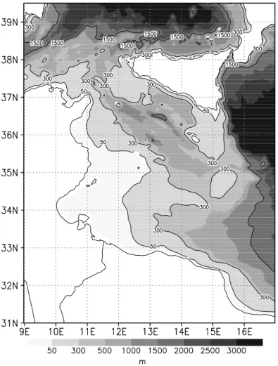
The Central Mediterranean is morphologically divided into two sub-areas, the Sar-dinia Channel at west and the Sicily Channel at east. They are separated by the Sicily Strait, a very shallow barrier for intermediate and deep waters due to an extension of the shelves from Cape Bon in Tunisia and Cape Lilibeo in Italy (Fig.1). The two chan-25

nels are crossed by the waters exchanging from the East and West Mediterranean basins and organized in a three-layer system from the surface to the bottom. Here the circulation is characterized, particularly at the surface, by strong mesoscale signals in the form of eddies, meanders and small-scale gyres whose path and lifetime are mainly

(5)

OSD

EGU influenced by the bathymetric contours, the temperature and salinity gradients, and the

meteorological conditions.

The upper ocean dynamics are dominated by the eastward flow of Modified Atlantic Water (MAW) which moves under the influence of the density gradient between the eastern and the western basin, and are modified by the influence of the wind forcing 5

and the bottom geometry. The MAW moves eastward from the Strait of Gibraltar along the north African coast forming unstable meanders that often originate from cyclonic and anticyclonic eddies with spatial scales of ∼200 Km (Puillat et al., 2002). From the Sardinia Channel two branches of MAW cross the Sicily Strait eastward. The first branch, the Atlantic Ionian Stream (AIS), moves along the south Sicilian coast as an 10

energetic and meandering flow (e.g.Robinson et al.,1999). Particularly evident in the summer, the AIS moves eastward in a complicated meandering path that, in the Sicily Channel, makes its flow around three surface thermal features: the Adventure Bank Vortex, the Maltese Channel Crest and the Ionian Shelf Break Vortex. The second branch, the African MAW current, moves along the Tunisian coast (Sorgente et al., 15

2003) and is characterized by high seasonal variability and a maximum volume trans-port in autumn (Manzella et al.,1988).

This paper is organized as follows: The first chapter gives a short description of the regional forecasting system, followed by a chapter with a presentation of the at-mospheric forcings used. After that, we show results of wind stress and sea surface 20

temperature assessment, followed by conclusions.

2 Methods

Here is an introduction to the SCRM forecast system, followed by a discussion about how the various atmospheric forcings are used in the present work. A description of the satellite data used for analysis is then presented.

(6)

OSD

EGU 2.1 Model setup

The SCRM forecasting system has been implemented over the Central Mediterranean sub-basin with a horizontal resolution of 1/32◦and 24 sigma layers in the vertical for a fine representation of the dynamical and physical processes. It is nested at the lateral open boundaries with the Ocean General Circulation Model (MFS1671) covering the 5

whole Mediterranean Sea. At the surface the SCRM is coupled with the mesoscale weather forecast system LAM2 for operational runs. Nesting is a useful technique that permits the simulation of small scale dynamics in a limited area using a high-resolution domain embedded in a lower resolution domain. This allows the large-scale structures generated on the coarse grid to influence the nested grid.

10

MFS1671 is the basin scale ocean model implemented on the whole Mediterranean basin with a horizontal resolution of 1/16◦and 72 fixed horizontal levels. The forecast system is based on the Ocean Parallelise Model (OPA) version 8.1, developed by the Laboratoire d’Oceanographie Dynamique et de Climatologie, Institute Pierre Simon Laplace, Paris. OPA is a primitive equation model. Navier-Stokes equations are used 15

with the approximation of thin-shell, Boussinesq, hydrostatic and incompressible fluid. A detailed description of the code can be found in Madec et al. (1998). MFS1671 provides analyses and forecasts in daily means centered at midnight. Its fields provide both the initial and lateral boundary condition for SCRM during the simulation period.

SCRM is based on the Princeton Ocean Model (POM), a three-dimensional, free sur-20

face ocean model that solves the equations of continuity, motion, conservation of tem-perature, salinity and assumes hydrostaticy and the Boussinesq approximation ( Blum-berg and Mellor,1987). The vertical mixing coefficients are calculated using theMellor and Yamada (1982) turbulence closure scheme, while the horizontal diffusion terms are calculated using the Smagorinsky formula (Smagorinsky, 1993). For the advec-25

tion of tracers,Smolarkiewicz(1984) scheme coded bySannino et al.(2002) has been used. The model uses a time splitting scheme for an efficient integration of internal (baroclinic) and external (barotropic) modes.

(7)

OSD

EGU The model grid extends from 9◦E to 17◦E and from 31◦N to 39.5◦N with a horizontal

resolution of 1/32◦ (∼3.5 km). There are 257×273 mesh points with 24 sigma levels; the barotropic time step is 4 s, while the baroclinic time step is 120 s.

The model bathymetry comes from the U.S. Navy Digital Bathymetric Data Base (DBDB1) at 1/60◦by bilinear interpolation into the model grid. Additional light smooth-5

ing is applied to reduce the sigma coordinate pressure gradient error (Mellor and Blum-berg,1986). The resulting model bathymetry is shown in Fig. 1. The maximum depth is ∼4000 m, while the minimum depth is set equal to 5 m.

The initial condition has been obtained using the forecasted daily mean fields of temperature, salinity and total velocity from MFS1671. In order to reduce the spin-up 10

time, which affects the forecast due to high frequency oscillations, data have been pro-cessed through variational initialization, named VIFOP. VIFOP ensures physical con-sistency of the fields and imposes the conservation of global divergence and the strong constraint on the sea surface elevation tendency (Auclair et al.,2000). For a more de-tailed description of VIFOP implementation on SCRM including sensitivity studies, see 15

Gaberˇsek et al.(2006).

SCRM is coupled at the lateral open boundaries with MFS1671, using a one-way asynchronous nesting of the forecasted daily mean fields of temperature, salinity and total velocity, imposing the interpolation constraint on the total velocity. This allows the total volume transport to be preserved after the interpolation procedures from the 20

coarse to the fine resolution model. The grid-nesting ratio between the coarse model and the regional ocean model is 2.0.

The regional model has three open boundaries located in the southern Tyrrhenian Sea (39.55◦N), in the Sardinia Channel (9◦E) and in the open Ionian Sea (17.1◦E). At these open boundaries, the normal and tangential barotropic velocity components at 25

each internal time step are fully specified by a bilinear interpolation of the daily mean forecasted fields from MFS1671 into the SCRM:

(8)

OSD

EGU

V_HR= V_LRint, (2)

where the subscripts HR and LR stand for high and low spatial resolution, respectively, while the superscript “int” marks the interpolated value. The normal barotropic veloc-ities are specified through the following equation, initially proposed byFlather (1976) and subsequently modified byMarchesiello et al.(2001) andPinardi et al.(2003): 5 ¯ U_HR= ¯U_LRint H+ η int LR H+ η_HR + ε s g H + η_HR(ηHR− η int LR), (3) with ¯ U_LRint= 1 H+ η_LR Zη −H U_LR d z. (4)

Here H is the bathymetry in the fine resolution, while η is the coarse free surface ele-vation interpolated with the fine model resolution. The term ε is equal to ±1 depending 10

of position of the open boundary; ε=+1 for the eastern and northern open boundary, ε=−1 for the western and southern open boundary. The tangential barotropic compo-nent velocities at the boundaries are simply equalized:

¯

V_HR= ¯V_LRint. (5)

To update the potential temperatureΘ and the salinity S at the open boundaries of 15

SCRM, an upstream advection scheme is used when the velocity is directed outward from the modeling area:

∂(Θ, S)_high

∂t + Uhigh

∂(Θ, S)_high

∂n =0, (6)

where n indicates the normal to the section. In cases of inflow through the open boundaries, the three-dimensional daily mean fields of temperature and salinity are 20

(9)

OSD

EGU prescribed from the values of the coarse model solution interpolated on the nested

open boundary: Θhigh= Θint

coarse (7)

S_high= S_coarseint . (8)

2.2 The atmospheric forcings 5

The model forecast skill depends on the quality and the way that surface boundary conditions are specified. At the surface, SCRM is driven by air/sea exchanges of heat, water and momentum, using the boundary conditions:

ρ₀C_pK_H ∂Θ ∂z z=η = Qtot (9) K_H ∂S ∂z _z_=η= (E − P )S (10) 10 ρ₀K_M ∂U ∂z z=η = τ, (11)

where ρ₀=1025 kg m−3is a reference density for marine water, C_p=4186 J kg−1K−1is the specific heat of pure water at constant pressure, K_H and K_M are the heat diffusivity the kinematic viscosity coefficient for water, respectively. On the left-hand side, the variation with depth z of potential temperatureΘ, salinity S and velocity U is always 15

evaluated at the surface (z=η). The right-hand side shows the source of variation for temperature, salt concentration and momentum, which are respectively the total heat flux Q_tot, the total salt flux (E −P )S and the wind stress τ, where E −P is evaporation minus precipitation. These three sources of air/sea interaction can be provided directly by the atmospheric model or can be calculated from primitive parameters such as air 20

(10)

OSD

EGU latter method had always been chosen when a flux relied on sea surface temperature,

for which we use SST simulated by the ocean model itself. In this sense, air/sea cou-pling is interactive. The parameters used are based onCastellari et al. (1998). In this paper we have summarized the essential points regarding parametrizations referring the reader to the previous reference for an extensive discussion and for the calculation 5

of the following physical quantities.

The total heat flux is divided into four parts:

Q_tot= Q_s− Q_b− Q_e− Q_h, (12)

where Q_s is the solar (shortwave) radiation flux, Q_b is the long wave radiation flux, Q_e is the latent heat flux, mainly due to the evaporative processes, and Q_h is the sensible 10

heat flux driven by a difference between air and sea surface temperature. We consider the fluxes Q_b, Q_eand Q_h positive for energy gained by the atmosphere. It is important to note that the shortwave flux has also an upward component (depending on albedo of the surface) while the longwave flux has also a downward component (depending on the radiation of the atmosphere).

15

The total salt flux depends on the surface salinity S simulated by the model and the water balance of air/sea exchanges. The evaporative flux E is related to the latent heat flux Q_eby

Q_e= L_eE, (13)

where L_eis the latent heat of evaporation for water. 20

Finally, the wind stress is parameterized as

τ= ρ_AC_DW , (14)

where ρ_Ais the density of moist air, C_Dis the drag coefficient and W is the wind vector. The AF used in this work to furnish the physical variables related to surface boundary conditions are:

(11)

OSD

EGU

– MR (medium resolution: 0.5◦, 6-hourly) model from European Centre for Medium-Range Weather Forecasts - ECMWF;

– HR (high resolution: 0.1◦, 1-hourly) Limited Area Model 2 – LAM2;

– VHR (very high resolution: 0.05◦, 1-hourly) Non-Hydrostatic model 1 – NH1. ECMWF runs a spectral, hybrid coordinate model, which produces 10-day fore-5

casts widely used by the scientific community together with hindcasts and historical re-analysis of atmospheric conditions. It is further described inSimmons et al.(1989) andCaplan et al.(1997). Forecasts are produced once a week, and for each day four atmospheric forecast snapshots at 00:00, 06:00, 12:00 and 18:00 UTC are given.

NH1 and LAM2 are both applications of the Skiron/Eta finite difference modeling 10

system described byKallos et al. (1997,2005), differing only in horizontal resolution. This limited-area, non-hydrostatic model produces forecasts over the entire Mediter-ranean Sea once a week, using the ARPEGE fields as initial and lateral boundary conditions. For each day, 24 atmospheric forecast snapshots at 00:00, 01:00, 02:00, . . ., 23:00 UTC are produced. Total precipitation is accumulated in hourly increments 15

(e.g., the file marked 05 contains the total precipitation accumulated from 04:00 to 05:00 UTC).

The characteristics and products of the various atmospheric models are summarized in Table1. In particular, note that ECMWF does not provide precipitation data, so for ECMWF-driven ocean simulations, the variable P in Eq. (10) is always set equal to 20

zero.

Weekly forecasts were produced in a so called slave mode, i.e. for each run SCRM is re-initialized using the initial boundary conditions provided by the basin scale model (MFS1671). Starting from the initial time SCRM produces a 5-day forecast run. For each atmospheric forcing, five separate runs were performed:

25

– RUN1 from 29 December 2004 to 2 January 2005; – RUN2 from 5 January 2005 to 9 January 2005;

(12)

OSD

EGU

– RUN3 from 12 January 2005 to 16 January 2005; – RUN4 from 19 January 2005 to 23 January 2005; – RUN5 from 26 January 2005 to 30 January 2005.

2.3 Data analysis

Ocean variables from the above runs have been validated against various remote-5

sensed datasets:

– Wind stress: daily mean data from SeaWinds scatterometer onboard QuikSCAT

satellite, quality checked and interpolated on a 1/2◦ grid by IFREMER-LOS/CERSAT (France);

– SST: sea surface temperature daily mean data from the 5-channel Advanced Very

10

High Resolution Radiometer AVHRR/3 sensor onboard NOAA-16 satellite; data have been quality checked and interpolated on a 1/16◦ grid by the ISAC-CNR – Istituto Studi Atmosfera e Clima (Italy).

Assessments of daily-mean model output have been performed and surface maps have been directly compared. Furthermore, we analyzed daily surface-averaged wind stress 15

magnitude, wind stress direction and sea surface temperature, which were then com-pared to averaged observed variables. Satellite data have then been interpolated on SCRM grid through bilinear interpolation, allowing the calculation of a root mean square error between forecasted and observed fields.

3 Results

20

3.1 Wind stress analysis and sea surface currents

Wind stress, calculated through bulk formulae from the wind field, is an additional input for the ocean model which was also analyzed. The availability of satellite scatterometer

(13)

OSD

EGU data made it possible to perform a preliminary validation of the wind stress field

sug-gesting it could possibly be the main reason for a different ocean response. The wind stress is a dominant atmospheric forcing for the 5-day ocean forecast experiments in a slave mode. It heavily influences both surface circulation and heat/water exchanges across the sea surface.

5

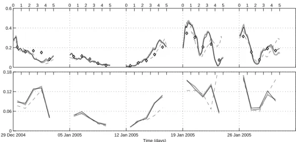
A global assessment of wind stress for the entire SCRM basin is shown in Figs.2 and3. The results show that, in general, both wind stress mean intensity and direction are forecasted well by all the atmospheric models in their variation in time. The root mean square error, which provides information about the fitting of fields, shows the forecast error of wind stress intensity is usually within 30% of the observed value, while 10

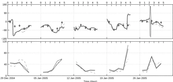
the wind stress direction is forecasted within 20◦.

In more detail, the top panel of Fig. 2 appears that the first three runs (RUN1-3) are characterized by slow and varying wind stress intensity. Additionally, the three AF are all similar and in good agreement with the satellite data. Differences between AF arise when a rapid change in time of wind stress field occurs. In the last two 15

forecast runs (RUN4-5) there were strong daily variations of wind magnitude. In this period, results show that mean magnitude is better forecasted by NH1 and LAM2. The same behavior appears by looking at wind stress direction (Fig. 3, top panel). The agreement with the satellite data is very good for all the AF for RUN1-3. It is noticeable that in this period there are still rapid changes in wind direction, from eastward to 20

south-westward in RUN1, between 29–30 December 2004. In contrast, in RUN4-5, the relative agreement is not as good since NH1 and LAM2 show bigger variations, both positive and negative, with respect to ECMWF forecasts. Therefore, it makes sense to analyze the period RUN1-3 separately from the period RUN4-5, to look for specific events that characterize these regimes. The analysis of wind stress will permit us to 25

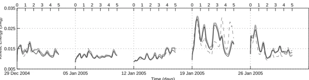
assess the ocean currents at the surface which are mainly wind-driven. The existence of the two distinct periods depicted above is confirmed by the sea surface dynamics and appears clearly in the time series of surface kinetic energy (Fig.4). During the RUN1-3 period, all three AF drove similar dynamics and produced almost constant

(14)

OSD

EGU kinetic energy of the surface layer. In the RUN4-5 period, the energy content suddenly

rose by 100% and oscillations became more intense, returning to values comparable with the RUN1-3 period only at the end of RUN5. A comparison with the time series of wind stress intensity, (Fig.2, top panel) shows the prompt response of the ocean model to the AF, which force a more energetic circulation if stronger wind intensity is 5

forecasted.

Regarding the RUN1-3 period the time series of the spatially averaged values of wind stress magnitude and direction show that NH1 and LAM2 have a similar behavior as confirmed by rmse time series. For wind stress magnitude, the most noticeable differences are in the last two days of RUN3, when the ECMWF forecast gives a lower 10

mean intensity with respect LAM2, making a better fit with satellite data. Regarding wind direction, HR and VHR AF practically have an identical behavior for the whole RUN1-3 period.

To gain further insight of the difference between AF we analyzed surface maps. For example, Fig.5shows the daily mean wind stress field over the Central Mediterranean 15

for the RUN1-3 period, forecasted and observed by a satellite for 5 January 2005 (start of RUN2). The results suggest the main features are forecasted well by every AF: (i) the prevailing north-westerly direction, (ii) the general magnitude, and (iii) the strongest winds over the open sea from Sardinia towards the south-east, reaching the maximum in front of Malta.

20

A lower wind stress intensity was also noticed, which was forecasted by ECMWF with respect to higher-resolution models, as already visible from means of Fig.2(top panel, start of RUN2). Regarding NH1 and LAM2, wind stress shows a very similar, general pattern for both AF. However, for wind blowing across an obstacle (land) the VHR model NH1 shows generally higher values of wind stress in the downwind region and a 25

longer extension of plumes. This is particularly visible in the south-east of the Messina Strait, where NH1 best fits with satellite data forecasting of a plume underestimated by LAM2 and totally omitted by ECMWF. Other regions in which this phenomenon is often remarkable with north-westerly wind (the most common in this region) are Malta Island

(15)

OSD

EGU and Cape Bon in Tunisia.

Analyzing the RUN4-5 period, differences in wind stress intensity and direction among the various forecasts are quite relevant, especially for the second half of the simulations, as appears in Figs.2and3. The biggest gap in wind stress intensity and direction pertain to 23 January 2005. During that day, the average satellite magnitude 5

of about 0.1 Nm−2 was well forecasted by NH1 and LAM2, whereas ECMWF provided a much larger value of 0.25 Nm−2. Also, for the same day, ECMWF gave a better fore-cast of the wind direction (south-eastward) while NH1 and LAM2 gave north-eastward winds. Another difference in wind stress intensity was visible for 30 January 2005, when the higher-resolution AF predicted values closer to satellite measurements. Moreover, 10

a clear difference between NH1 and LAM2 was visible with NH1 giving a mean inten-sity greater by 30% with respect to LAM2 and was more consistent with satellite data. Regarding wind direction, NH1 and LAM2 had practically identical behavior for all the forecast runs, except during RUN5, on 28 January 3rd forecast day). In the first hours of that day the dominant eastward wind rapidly changed its direction, becoming south-15

ward for NH1 or northward for LAM2 at 05:00 UTC and then approximately returning to its previous direction. In contrast, ECMWF forecasts produced a steady eastward wind during the same period. Rmse in that day was quite high (∼70◦) for all AF, but consider that there was the same problem of resolution with satellite data, which are daily means not useful to show similar fast events. In any case, Fig.2 suggests that 20

the differences appeared in a period of very low winds.

The differences in forecasted wind field influenced the sea surface current (SSC). For example, the SSC for 23 January 2005, indicates a maximum discrepancy between ECMWF and NH1-LAM2, as discussed above (Fig.6). Before analyzing SSC di ffer-ences, the general behavior of the eastward MAW flux was observed. It was clearly 25

detectable as a strong velocity stream emerging from Sardinia Channel and dividing in two main branches at the Sicily Strait. The northern branch propagated eastward in a meandering way, passing between Sicily and Malta and the southern branch went south-eastward, approximately following the 50 m bathymetry (Fig.1), producing

(16)

vari-OSD

EGU ous vortices during its passage.

Figure 6compares SCRM current forecasts obtained with by using various AF and with MFS1671 forecast. MFS1671, as explained in Sect. 2, is the coarser resolution ocean model from which SCRM takes the initial and boundary conditions. The atmo-spheric fields are provided by the same medium resolution AF (ECMWF) as used for 5

SCRM. Therefore, it is not surprising that SSC, forced by ECMWF, are quite similar for both ocean models SCRM and MFS1671 (bottom panels of Fig.6). On one hand there are differences like the small vortex to the north of Messina Strait, which are ascribed to the higher resolution of the ocean model itself (1/32◦ for SCRM against 1/16◦for MFS1671). On the other hand, SSC forecasts produced by higher-resolution 10

AF show remarkable differences from the ECMWF-driven forecast. As expected from wind stress intensities, which were closer to observations for higher-resolution AF, sea surface circulation is less intense for NH1 and LAM2. It presents more vortices, espe-cially in the shallow Gulf of Gabes and in the triangle of Sardinia-Sicily-Tunisia, probably due to the different direction of winds from the various AF.

15

As already noted, another characteristic event was the difference in forecasted wind stress direction for 28 January 2005. The relative maps of wind stress are shown in Fig. 7, representing snapshots at 06:00 UTC for NH1, LAM2 and ECMWF, and daily mean for satellite observation. It turns out that the differences in mean wind stress di-rection between AF were due to the passage of a fast cyclonic disturbance located near 20

the northern boundary. A vortex formed south-east of Sardinia and crossed eastward of the SCRM domain in about 12 h. The structure was fully developed in NH1 while LAM2 showed only a very weak trace of this phenomenon and it was not visibile using ECMWF. Differences between NH1 and LAM2 are probably caused by the enhanced description of orographyc features in NH1 due to its greater spatial resolution, while the 25

ECMWF resolution was lower than LAM2 and does not reproduce the phenomenon at all. Unfortunately, satellite observations cannot aid to assess the reality of that event due to their daily resolution. It is interesting to note, by observing closely the surface kinetic energy for 28 January 2005 (Fig. 4, RUN5), that NH1 presented a peak with

(17)

OSD

EGU respect to LAM2 which is centered on 17:00 UTC. This was produced by the

afore-mentioned 05:00 UTC perturbation showing that the delay of SSC in response to wind changes is about 12 h. In any case, the event was so fast and weak that daily mean SSC for this day did not present any difference between the various AF (not shown). 3.2 Sea surface temperature analysis

5

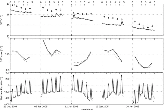
SST is the most important parameter to validate an ocean forecast over an extended domain, provided the existence of sufficiently high resolution satellite observations. The assessment of SST on SCRM domain is shown in Fig. 8, showing mean SST, its rmse with respect to satellite data, and the net ocean heat flux which drives the changes of temperature. The temporal variations of mean values (top panel), were well 10

followed by ocean model whatever AF is used, but they generally underestimated the observed SST for about 0.5◦C. The gap between forecasts and observations remained approximately the same for the whole analyzed period, in which the sea cools at the surface from 17◦C to 15◦C, approaching its lowest annual value (usually about 14◦C, reached at the end of February).

15

The diurnal cycle is also visible (Fig.8), occasionally reaching large oscillations, as in the first day of RUN3 and in the fifth day of RUN4 (23 January 2005), when there was a difference of about 0.3◦C between the minimum and maximum value of the spatially averaged SST. In those dates there was also the most noticeable difference between AF, with NH1 and LAM2 giving warmer temperatures (+0.2◦C) with respect to ECMWF 20

and approaching the remote-sensed values.

The intense oscillations of SST are related to the maximum day/night differences in the net heat flux exchange between air and sea (Fig.8, bottom panel). The heat loss occurs most of the time, with the occasional heat gain only during the daytime. Dif-ferences in heat flux between ECMWF and higher-resolution AF are often quite large 25

during the daytime, probably due to the parameterization for solar radiation when using ECMWF, which relies basically on geometric considerations (see Table 1). Alterna-tively, solar radiation fluxes were directly provided by NH1 and LAM2 with a

(18)

presum-OSD

EGU ably better parameterization. Other sources of divergence for heat fluxes were the

wind intensity (biggest heat losses are closely related to strong wind periods, compare with Fig.2) and the air temperature (not shown), affecting the latent and sensible heat fluxes. The variation was more clearly visible during the night time, when the solar en-ergy flux is zero. Nonetheless, the different net heat fluxes cannot produce a marked 5

variation in SST, provided the slow variation of temperature with time, and recalling that forecasts are run in slave mode. The weekly re-initialization based on the coarse model forces SCRM to stay close to the prescribed initial boundary conditions. This is ever more apparent for NH1 and LAM2, which differ only in horizontal resolution and which produce identical SST time series.

10

The rmse analysis (Fig.8, center panel) shows quite large variations in the skill of the model predicting the SST, ranging from 0.5◦C to 1◦C. Minimum values are reached during RUN5, when also the spatially averaged SST are more similar. The slightly lower ECMWF rmse (generally 0.03◦C lower than NH1 and LAM2) is compensated by the error on satellite SST (usually around 4% of the estimated value).

15

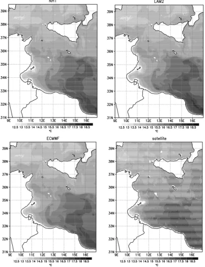
The SST pattern is mainly influenced by geographical position (through the modu-lation of solar radiation with latitude) and by the presence of circumodu-lation patterns like eddies and coastal upwellings. As an example, both forecasted and observed SST distribution, for 23 January 2005 are shown in Fig. 9. During that day there was the maximum discrepancy in the mean SST between the various AF, as noted above. The 20

general pattern shows an increasing temperature toward the south-eastern portion of the domain, modulated by local features. Among these, it is worthy to note the southern branch of MAW characterized by low temperatures along the African shelf. In partic-ular, the lowest SST were reached in the Gulf of Gabes (southern Tunisia); this is a large area in which the temperature variations reach the extremes, due to its shallow-25

ness (depth <50 m). The ocean model had a very good response in this area when compared to satellite SST data, independently from the AF used. Another feature well resolved by all the AF is the cold region next to the southern Italian coast of Sicily and Calabria, due to extended coastal upwellings induced by the northern branch of

(19)

OSD

EGU MAW and the large region of warm water standing off the northern African coast below

35◦N. Conversely, the main differences between model forecasts and observations are the SST underestimation of the large system of warmer water of the Ionian Ther-mal Front which, starting from 36◦N, extends northward reaching the eastern offshore of Sicily. Another different pattern is the warmer region north-west of Malta, which is 5

clearly seen by satellite but missing in forecasts.

The temperature patterns produced by different AF result in a very similar SST distri-bution on a daily basis. In Fig.9only minor differences are visible among the forecasted and observed SST. As already noted above, it is a limit of the slave-mode forecasts, in which sometimes large differences in heat fluxes provided by the various AF do not 10

have sufficient time to affect SST.

4 Conclusions

In this paper we have analyzed the response of a regional ocean forecasting sys-tem, operating in near real time on the Central Mediterranean, driven by three different atmospheric models. The atmospheric forcings used had an increasing resolution, 15

temporal (from 6-h to 1-h) and spatial (from 0.5◦ to 0.05◦). The two higher-resolution forcings were both applications of the same atmospheric model (differing only in hori-zontal resolution), while the medium-resolution forcing has been provided by a different model. For each of the five chosen time periods, ocean forecasts have been obtained from three different simulations, differing in atmospheric forcing. Each run started in 20

slave mode, i.e. initializing the regional model according to the initial and boundary ocean conditions provided by a coarser ocean model. Forecasts have been assessed by satellite data, using as a reference a set of remote-sensed measurements of wind stress and sea surface temperature.

The analysis suggests that all the atmospheric forecasts give in general a good es-25

timation of wind field, both in intensity and direction. When marked differences in wind forecasts arise, the ocean model responds promptly resulting in different sea

(20)

OSD

EGU surface dynamics. In general, all the produced sea surface current patterns seem

to be in agreement with the present knowledge of the circulation in the area. The higher-resolution forcings often drive current patterns with more vortices. The very high-resolution forcing, in particular, has been the only model able to predict the fast passage of a small cyclonic perturbation in the Sardinia Channel, which affected the 5

surface circulation in the area during the following hours. Unfortunately, no direct com-parison with measured surface current were possible, due to the lack of measurements. The wind stress assessment, which indirectly gives information on the sea current fore-cast skill, was not conclusive to clearly distinguish between the various atmospheric forcings, due to the low resolution (both spatial and temporal) of the satellite data used 10

as reference.

Sea surface temperature is in a good agreement with the satellite data, though ocean model in general underestimates it for about 0.5◦C. Regardless, the surface patterns of temperature are essentially in agreement with measured ones, showing the thermal track of well-known structures. At the same time, no remarkable differences in the 15

surface temperature forecast skill arise using the various atmospheric forcings.

Within the scope of this work, higher-resolution atmospheric forcings have shown the ability to form interesting dynamics structures on surface, though no direct assess-ment of currents was possible. The sea surface temperature remains substantially unaffected by the change of atmospheric model. In this regard, an important point to 20

note is that the ocean model was run in slave mode. In fact, this kind of system gives essentially no time for the regional model to develop its own dynamics on larger scales, forcing it to stay closer to the results of the coarse model. In this way, the various sur-face dynamics features that have been noticed emerging when forecasted wind fields were different, are constrained to have a short life. It is also known how important are 25

the precise hour-by-hour surface current forecasts in an application such as the oil-spill modeling, especially when operatively used for emergencies, or in general for the dis-persion of pollutants in the sea. Besides this, possibly different air/sea fluxes, arising for example from different wind intensity or air temperature forecasts, have no time to

(21)

OSD

EGU produce effects on slowly-changing variables like sea surface temperature.

These problems could in principle be avoided running ocean forecasts in active mode, i.e. restarting regional model without re-initialization by the coarse model. This implies the temporal continuity of atmospheric forcings. The comparison of the effect of different atmospheric forcings under such an active forecast system will be the future 5

development of this work, together with the extensive use of experimental data from current meter gauges to directly test the reliability of sea surface current forecasts.

Acknowledgements. This work has been realized in the framework of EU MFSTEP project

(EVK3-2001-00174) and the EU Marie Curie host fellowship: ODASS project (HPMD-CT-2001-00075). In the framework of EC MFSTEP project, atmospheric forcings have been produced

10

by IASA institute (GR) for Skiron NH1 and LAM2, and ECMWF (UK). Coarse ocean model data are due to INGV (IT), which we also thank for general coordination of MFSTEP project. Satellite daily SST data are produced by ISAC-CNR (IT), while wind stress satellite data are due to the department LOS/CERSAT of IFREMER (FR).

References

15

Auclair, F., Marsaleix, P., and Estournel, C.: Sigma Coordinate Pressure Gradient Errors: Eval-uation and Reduction by an Inverse Method, J. Atmos. Ocean. Tech., 17(10), 1348–1367, 2000. 642

Bignami, F., Marullo, S., Santoleri, R., and Schiano, M. E.: Longwave radiation budget in the Mediterranean Sea, J. Geophys. Res., 100(C2), 2501–2514, 1995. 660

20

Blumberg, A. F. and Mellor, G.: A description of a three-dimensional coastal ocean circulation model, Three-dimensional Coastal Ocean Models, Coastal Estuarine Science, edited by: Heaps, N. S., Americ. Geophys. Union, 1–16, 1987. 641

Caplan, P., Derber, J., Gemmil, W., Hong, S. Y., Pan, H. L., and Parrish, D.: Changes to the 1995 NCEP Operational Medium-Range Forecast Model Analysis Forecast System, Weather

25

and Forecasting: 12(3), 581–594, 1997. 646

Castellari, S., Pinardi, N., and Leaman, K.: A model study of air-sea interaction in the Mediter-ranean Sea, J. Mar. Syst., 18, 89–114, 1998. 645,660

(22)

OSD

EGU

Castellari, S., Pinardi, N., and Leaman, K.: Simulation of water mass formation proces in the Mediterranean Sea: Influence of the time frequency of the atmospheric forcing, J. Geophys. Res., 105(C10), 24 157–24 181, 2000. 639

Flather, R. A.: A tidal model of the northwest European continental shelf, Mem. Soc. R. Sci. Liege, 6(X), 141–164, 1976. 643

5

Gill, A. E.: Atmospheric-Ocean Dynamics, Academic Press, 1982. 660

Gaberˇsek, S., Sorgente, R., Natale, S., Ribotti, A., Olita, A., Astraldi, M., and Borghini, M.: The Sicily Channel Regional Model forecasting system: initial boundary conditions sensitivity and case study evaluation, Ocean Sci. Discuss., 3, 221–254, 2006. 642

Hellerman, S. and Rosentein, M.: Normal wind stress over the world ocean with error estimates,

10

J. Phys. Ocean., 13,1093–1104, 1983. 660

Herbaut, C., Martel, F., and Cr ´epon, M.: A sensitivity study of the general circulation of the Western Mediterranean Sea. Part II: the response to atmospheric forcing, J. Phys. Oceanogr., 27, 2126–2145, 1997. 639

Jerlov, N. G.: Marine Optics, Elsevier, 1976.

15

Kallos, G., Nickovic, S., Papadopoulos, A., Jovic, D., Kakaliagou, O., Misirlis, N., Boukas, L., Mimikou, N., Sakellaridis G., Papageorgiou J., Anadranistakis, E., and Manousakis, M.: The regional weather forecasting system Skiron: An overview, Proceedings of the Symposium on Regional Weather Prediction on Parallel Computer Environments, 109–122, 15–17 October 1997, Athens, Greece, 1997. 646

20

Kallos, G., Pytharoulis, I., and Katsafados, P.: Limited Area Weather Forecasting for the MF-STEP activities: Sensitivity and Performance Analysis, 4th EuroGOOS, Brest, France, 2005. 646

Kondo, J.: Air Sea bulk transfer coefficients in adiabatic conditions, Boundary-Layer Meteorol., 9, 1573–1472, 1975. 660

25

Madec, G., Delecluse, P., Imbard, M., and Levy, C.: OPA8.1 Ocean general Circulation Model reference manual, Note du Pole de modelisazion, Institut Pierre-Simon Laplace (IPSL), France, 1998. 641

Manzella, G. M. R., Gasparini, G. P., and Astraldi, M.: Water exchange between the eastern and western Mediterranean through the Strait of Sicily, Deep-Sea Res., 35, 1021–1035,

30

1988. 640

Marchesiello, P., Mc Williams, J. C., and Shchepetkin, A.: Open boundary conditions for long-term integration of regional oceanic models, Ocean Modeling, 3, 1–20, 2001. 643

(23)

OSD

EGU

Martellucci, A., Poiares Baptista, J. P. V., and Blarzino, G.: New climatological databases for Ice depolarisation on satellite radio links, COST Action 280 1st international workshop, PM3037, July, 2002. 660

Mellor, G. L. and Blumberg, G.: Modeling vertical and horizontal diffusivities with a sigma coordinate system, Mon. Weather Rev., 113, 1279–1383, 1986. 642

5

Mellor, G. L. and Yamada, T.: Development of a turbulence closure submodel for geophysical fluid problems, Rev. Geophys. Space Phys., 20, 851–875, 1982. 641

Payne, R. E.: Albedo of the sea surface, J. Atmos. Sci., 29, 959–970, 1972. 660

Pinardi, N., Allen, I., Demirov, E., De Mey, P., Korres, G., Lascaratos, A., Le traon, P. Y., Maillard, C., Manzella, G. M. R., and Tziavos, C.: The Mediterranean ocean forecasting system: first

10

phase of implementation, Ann. Geophys., 21, 3–20, 2003. 638,639,643

Puillat, I., Taupier-Letage, I., and Millot, C.: Algerian eddies lifetime can near 3 years, J. Mar. Syst., 31, 245–259, 2002. 640

Reed, R. K.: On estimating insolation over the ocean, J. Phys. Oceanography, 7(3), 482–485, 1977. 660

15

Robinson, A. R., Sellschopp, J., Warn-Varnas, A., Anderson, L. A., and Lermusiaux, P. F. J.: The Atlantic Ionian Stream, J. Mar. Syst., 20, 129–156, 1999. 640

Rosati, A. and Miyakoda, K.: A general circulation model for the upper ocean simulation, J. Phys. Oceanogr., 18(11), 1601–1626, 1988. 660

Sannino, G. M., Bargagli, A., and Artale, V.: Numerical modelling of the mean exchange through

20

the Strait of Gibraltar, J. Geophys. Res., 107(CB) Ant. No. 3094, doi:10.1029/2001JC000929, 2002. 641

Simmons, A. J., Burridge, D. M., Jarraud, M., Girard, C., and Wergen, W.: The ECMWF medium-range prediction models development of the numerical formulations and the impact of increased resolution, Meteorol. Atmos. Phys., 40(1–3), 28–60, 1989. 646

25

Smagorinsky, J.: Some historical remarks on the use of nonlinear viscosities, in: Large eddy simulations of complex engineering and geophysical flows, edited by: Galperin, B. and Orszag, S., Cambridge Univ. Press, 1993. 641

Smolarkiewicz, P. K.: A fully multidimensional positive definite advection transport algorithm with small implicit diffusion, J. Comput. Phys., 54, 325–362, 1984. 641

30

Sorgente, R., Drago, A. F., and Ribotti, A.: Seasonal variability in the Central Mediterranean Sea circulation, Ann. Geophys., 21, 299–322, 2003. 640

(24)

OSD

EGU

model studies of the Adriatic Sea circulation, Seasonal variability, J. Geophys. Res., 107, Ant. No. 3004,doi:10.1029/2000JC000210, 2002.

(25)

OSD

EGU Table 1. Atmospheric forcings used in this work and their variables. A provided field is marked

with√; otherwise, the field is calculated following the indicated reference. Bulk formulae used for fluxes are described byCastellari et al.(1998). NH1 and LAM2 provide the same fields with different horizontal resolution.

Parameter NH1-LAM2 ECMWF

Horizontal resolution NH1: 0.05◦; LAM2: 0.1◦ 0.5◦

Temporal resolution 1 h 6 h

Temporal coverage 5 days 10 days

Mean sea level pressure √ √

Cloud coverage √ √

Zonal wind at 10 m a.s.l. √ √

Meridional wind at 10 m a.s.l. √ √

Relative humidity at 2 m a.s.l. √ Martellucci et al.(2002) Specific humidity at 2 m a.s.l. not calculated √

Precipitation √ not provided

Drag coefficient Hellerman and Rosenstein(1983) Hellerman and Rosenstein(1983) Zonal wind stress Castellari et al.(1998) Castellari et al.(1998)

Meridional wind stress Castellari et al.(1998) Castellari et al.(1998)

Downward shortwave flux √ Rosati and Miyakoda(1988),Castellari et al.(1998) Upward shortwave flux √ Reed (1977),Payne (1972)

Downward longwave flux √ Bignami et al.(1995) Upward longwave flux Bignami et al.(1995) Bignami et al.(1995) Latent heat of vaporization Gill(1982) Gill(1982)

Latent heat flux Gill(1982),Kondo(1975) Gill(1982),Kondo(1975) Sensible heat flux Kondo(1975) Kondo(1975)

(26)

OSD

EGU Fig. 1. SCRM domain and bathymetry.

(27)

OSD

Printer-friendly Version Interactive Discussion EGU 0 0.2 0.4 0.6 τ magnitude (Nm −2 ) 0 1 2 3 4 5 0 1 2 3 4 5 0 1 2 3 4 5 0 1 2 3 4 5 0 1 2 3 4 5

29 Dec 20040 05 Jan 2005 12 Jan 2005 19 Jan 2005 26 Jan 2005 0.06 0.12 0.18 τ magnitude rmse (Nm −2 ) Time (days)

Fig. 2. Top: mean wind stress magnitude, forecasted and observed. Bottom: rmse of wind

stress magnitude with respect to satellite data. The solid thick light grey line represents NH1, solid thin black line LAM2, dashed dark grey line ECMWF and diamonds satellite data.

(28)

OSD

Printer-friendly Version Interactive Discussion EGU −180 −90 0 90 180 τ direction ( o) 0 1 2 3 4 5 0 1 2 3 4 5 0 1 2 3 4 5 0 1 2 3 4 5 0 1 2 3 4 5

29 Dec 20040 05 Jan 2005 12 Jan 2005 19 Jan 2005 26 Jan 2005 40 80 120 τ direction rmse ( o) Time (days)

Fig. 3. Top: mean wind stress direction, forecasted and observed. Bottom: rmse of wind stress

direction with respect to satellite data. Symbols are the same as in Fig. 2. Convention on directions is: wind blowing southward=−90◦; eastward=0◦; northward=90◦; westward=180◦.

(29)

OSD

EGU 29 Dec 2004 05 Jan 2005 12 Jan 2005 19 Jan 2005 26 Jan 2005

0.005 0.015 0.025 0.035 Kinetic Energy (J/kg) Time (days) 0 1 2 3 4 5 0 1 2 3 4 5 0 1 2 3 4 5 0 1 2 3 4 5 0 1 2 3 4 5

(30)

OSD

EGU Fig. 5. Forecasted and observed wind stress for 5 January 2005. For clarity, not all grid points

(31)

OSD

EGU Fig. 6. Streamlines of forecasted sea surface currents for 23 January 2005.

(32)

OSD

EGU Fig. 7. Forecasted and observed wind stress for 28 January 2005. Top, and bottom left:

forecasts for 06:00 UTC. For clarity, not all grid points have been plotted. Bottom right: mean of satellite observations 00:00–24:00 UTC.

(33)

OSD

Printer-friendly Version Interactive Discussion EGU 14 15 16 17 SST ( o C) 0 1 2 3 4 5 0 1 2 3 4 5 0 1 2 3 4 5 0 1 2 3 4 5 0 1 2 3 4 5 0.5 0.75 1 SST rmse ( o C)

29 Dec 2004−600 05 Jan 2005 12 Jan 2005 19 Jan 2005 26 Jan 2005 −400

−200 0 200 400

Net Heat Flux (Wm

−2

)

Time (days)

Fig. 8. Top: Mean SST, forecasted and observed. Center: rmse of SST with respect satellite

(34)

OSD

EGU Fig. 9. Forecasted and observed SST for 23 January 2005.