Forecasting circulation in the Cilician Basin of the Levantine Sea

(1)

HAL Id: hal-00298419

https://hal.archives-ouvertes.fr/hal-00298419

Submitted on 11 Sep 2006

HAL is a multi-disciplinary open access

archive for the deposit and dissemination of sci-entific research documents, whether they are pub-lished or not. The documents may come from teaching and research institutions in France or abroad, or from public or private research centers.

L’archive ouverte pluridisciplinaire HAL, est destinée au dépôt et à la diffusion de documents scientifiques de niveau recherche, publiés ou non, émanant des établissements d’enseignement et de recherche français ou étrangers, des laboratoires publics ou privés.

Forecasting circulation in the Cilician Basin of the

Levantine Sea

E. Özsoy, A. Sözer

To cite this version:

E. Özsoy, A. Sözer. Forecasting circulation in the Cilician Basin of the Levantine Sea. Ocean Science Discussions, European Geosciences Union, 2006, 3 (5), pp.1481-1514. �hal-00298419�

(2)

OSD

3, 1481–1514, 2006

Cilician Basin forecasting

E. ¨Ozsoy and A. S ¨ozer

Title Page Abstract Introduction Conclusions References Tables Figures J I J I Back Close Full Screen / Esc

Printer-friendly Version Interactive Discussion

EGU Ocean Sci. Discuss., 3, 1481–1514, 2006

www.ocean-sci-discuss.net/3/1481/2006/ © Author(s) 2006. This work is licensed under a Creative Commons License.

Ocean Science Discussions

Papers published in Ocean Science Discussions are under open-access review for the journal Ocean Science

Forecasting circulation in the Cilician

Basin of the Levantine Sea

E. ¨Ozsoy and A. S ¨ozer

Institute Marine Sciences, Middle East Technical University, Erdemli-Mersin, Turkey Received: 31 May 2006 – Accepted: 21 June 2006 – Published: 11 September 2006 Correspondence to: E. ¨Ozsoy (ozsoy@ims.metu.edu.tr)

(3)

OSD

3, 1481–1514, 2006

EGU

Abstract

The Cilician Basin/Shelf Model is adapted for studying the shelf circulation in the Cili-cian Basin – Gulf of ˙Iskenderun region of the Levantine Basin of the Eastern Mediter-ranean between the Turkish MediterMediter-ranean coast, Syria and the island of Cyprus. The model initial conditions and open boundary conditions are supplied by the ALERMO

5

regional model of the Levantine Sea, while interactive surface flux boundary condi-tions are specified by an atmospheric boundary layer sub-model using calculated wa-ter properties and surface atmospheric variables supplied by the Skiron atmospheric model, within the nested modelling approach of the MFSTEP (Mediterranean Fore-casting System: Towards Environmental Predictions) project. Sensitivity tests are

per-10

formed for alternative surface boundary conditions. Model performance for shelf/meso-scale forecasts is demonstrated.

1 Introduction

The Cilician Basin coastal system occupies the northeastern part of the Eastern Mediterranean Levantine Basin between Cyprus and Turkey, and includes the wide,

15

shallow continental shelf areas of Mersin and ˙Iskenderun Bays (Fig. 1). The continental shelf adjoining Mersin and ˙Iskenderun Bays is one of the widest in the entire Levantine Sea (excluding the Nile Cone) where the coastal bathymetry is often very steep. Taurus and Amanos mountain ranges bound the Cilician Basin respectively in the north and east, lined with narrow “riviera” coastal plains except in the vast delta plains of the

Sey-20

han and Ceyhan Rivers northwest of ˙Iskenderun Bay. The regional climate is typical of the Eastern Mediterranean, with hot, humid summers and rainy, mild winters, and short transitional seasons. Northerly winds dominate the winter (November to March), and a sea-breeze system with southwesterly winds dominate the summer (April to Oc-tober). Weather steered by steep mountain ranges but intercepted by valleys along

25

(4)

of-OSD

3, 1481–1514, 2006

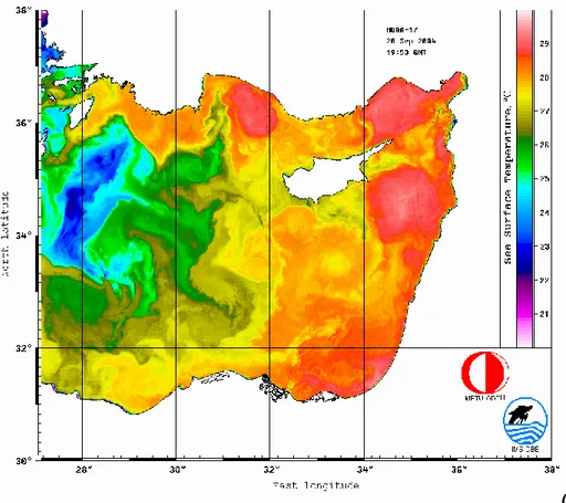
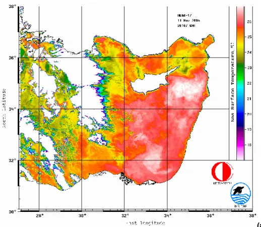
EGU ten develops local gale force winds in winter (Reiter 1975; ¨Ozsoy, 1981). Eddies and

meanders, wind driven currents, topographic/continental shelf waves, inertial/internal oscillations add significant variability to the basic cyclonic circulation exemplified by the satellite SST (Fig. 2a), the bifurcating mid-basin jet and the Asia-Minor current along the Turkish coast, interspersed with quasi-permanent anticyclonic eddies in the

5

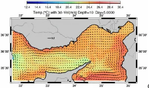
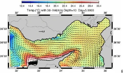
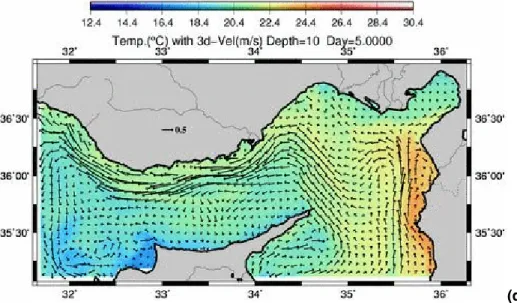
Eastern Mediterranean (W ¨ust, 1961; The POEM Group, 1992; ¨Ozsoy et al., 1993). Focusing on the Cilician Basin with the nested model simulations (Fig. 2b) described in the sequel, produces similar features to those observed via satellite. The classical picture of surface circulation in the Gulf of ˙Iskenderun after Collins and Banner (1979) aided by satellite imagery and unpublished observations of IMS-METU in the region

10

are schematized in Fig. 2c. Two main types of circulation were observed within the ˙Iskenderun Bay: in summer, two counter rotating eddies driven by surface currents entering west of the Bay were inferred, while in winter it was supposed that the cur-rents following the eastern coast could enter east of the Bay. Less saline and cooler waters were observed in the inner part of the Bay. Direct current measurements

car-15

ried out in winter 1992 indicated several high frequency oscillations in addition to an oscillation of about eight days period with current speeds in the range of 5–25 cm/s. The Cilician Basin coastal system is presently experiencing significant environmental stresses as a result of explosive increases in population, industrial, agricultural and tourism activities. Wastes from industries (steel, paper, fertilizer etc.) and untreated or

20

primary-treated municipal wastes from major towns of Mersin, Adana, ˙Iskenderun and Antakya are potential sources of marine pollution. Civilian and military marine trans-port linked to the harbours of Mersin, ˙Iskenderun and Tas¸ucu, oil storage and pipeline terminals at Yumurtalık, Ceyhan and D¨ortyol (including the recently completed Baku-Tblisi-Ceyhan pipeline transporting oil and gas from the Caspian Sea) are additional

25

activities with potential impact on the environment. Perennial rivers G ¨oksu, Lamas, Tarsus, Seyhan, Ceyhan and Asi plus some smaller rivers account for a total fresh water flux of 27 km3/yr (870 m3/s), accounting for about half the river discharge along the Turkish Mediterranean – Aegean coasts, but much greater than the present

(5)

dis-OSD

3, 1481–1514, 2006

EGU charge of the Nile in the Eastern Mediterranean (estimated to be 540 m3/s, Pinardi et

al., 2005). Following the almost 90% reduction in the discharge of the River Nile in the 1960’s, Turkish rivers concentrated in the Cilician Basin presently seem to be the main fresh water and nutrient sources for the entire Levantine Basin of the oligotrophic Eastern Mediterranean. Because of the significant inputs of these rivers, the Cilician

5

Basin has all the characteristics of the ROFI (regions of freshwater influence) but in the oligotrophic environment typical of the Eastern Mediterranean Sea.

2 Cilician Basin/Shelf circulation modeling

The Cilician Basin/Shelf Model domain covers the area shown in Fig. 1, with the hor-izontal grid characteristics given in Table 1, with a uniform nominal horhor-izontal grid

10

resolution of 1.35 km in both directions, and vertical resolution of 28 sigma levels. The external and internal integration time steps were ∆t_e=2 s and ∆t_i=40 s respec-tively, and model constants were: horizontal mixing coefficients A_m=A_h=200 m2/s, ini-tial vertical mixing coefficients K_m=K_h=K_s=2×10−4m2/s respectively for momentum, heat, salt and bottom roughness parameters z₀=0.01, C_b,min=0.0025. The fine scale

15

model bathymetry was generated from contour data of UNESCO bathymetric maps of Mediterranean, making limited use of the US Navy DBDB1 gridded bathymetry to fill ar-eas shallower than 50 m where contour data were missing. The model bathymetry was then filtered with a selective filter that smoothes only the steep slope areas so that the

r-value r=∆H/(2H) (where H is the depth) between adjacent grid points remains below

20

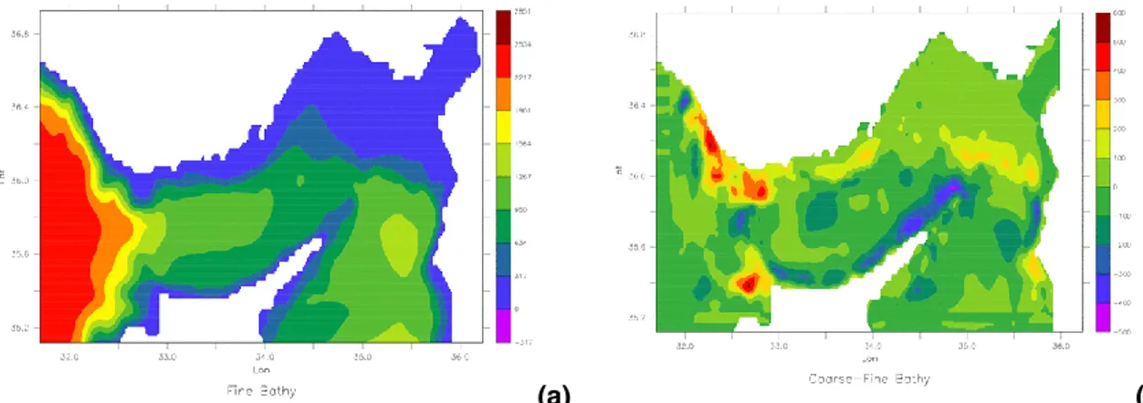
r=0.2. There were large differences between the coarse grid ALERMO bottom

topog-raphy and the fine grid Cilician Basin model bottom topogtopog-raphy (Fig. 3), which were even larger before the bathymetry data of the former was improved. In general, the Gulf of ˙Iskenderun shelf area was deeper in the coarse grid, while the area surround-ing the northeastern tip of Cyprus was shallower in the coarse grid. These differences

25

(6)

OSD

3, 1481–1514, 2006

EGU The bathymetry at about 10 rows of grids at open boundary sections were taken to be

exactly the same as the coarse model, regardless of the fine topography created, in order to conserve volume fluxes and transport properties between the coarse and fine grid models, and gradually melded into the interior fine topography.

The interpolation to the fine grid point from the surrounding eight coarse grid data

5

points (or the number of available points) was made by weighted averaging using the following weights at each of the eight coarse grid points:

W_k(x, y, z)= exp −[(x_c−x_f)2+ (y_c−y_f)2/s2_h]. exp −[(z_c−z_f)2/s_v2], k=1, 8

where s_hand s_vare scales for horizontal and vertical influences respectively and x, y, z are coordinates with subscript c indicating the coarse and f indicating the fine grid

10

points. Because both the coarse and fine grid coordinates are originally in sigma coor-dinates, the vertical scale s_v was locally adjusted to be representative of the average vertical distance between the coarse grid points, so that more uniform weighting was obtained in the shallow area as compared to the deep area. Because the coarse grid widely differs from the fine grid, especially near the bottom and the coast, special

15

care was taken for interpolation near these areas. The few coastal points outside the coarse domain were extrapolated from data at the same depth. The deep data outside the coarse domain were interpolated from the data above its depth using the above 8 point scheme but including only those points where there were data available. The effect of this scheme is to replace data points with values available in the upper layers,

20

and seemed to be performing well considering the rather uniform properties at great depth. The bottom values from the coarse model (the last vertical grid point) were values not used by the model, and therefore eliminated from the interpolation. Data availability near the bottom was an issue that strongly affected interpolation, because the coarse grid domain was often shallower than the fine grid domain in shelf regions.

25

At intermediate depths this is not a very severe problem, because data are only miss-ing in limited areas such as near the coasts and the vicinity of the sharp northeast Cape of Cyprus. At the bottom layer of the fine grid the number of data available for interpolation from the lower layer decreases greatly, due to the shallower limits of the

(7)

OSD

3, 1481–1514, 2006

EGU coarse domain in same areas. The data in those areas were filled mostly by

inter-polation from the data available in the upper layer. Open boundary conditions tested for nested domains in the Mediterranean Forecasting System MFS (e.g. papers in De Mey et al., 2003 special volume for MFS), namely the specification of barotropic flow velocity with a radiation component on the normal component (Flather b.c.), baroclinic

5

velocity components and temperature/salinity with advective conditions during outflow have been adopted in the present model. Instantaneous momentum, heat and salt flux boundary conditions at the sea surface,

K_m(d u/d z)= T_x,

10

K_m(d v /d z)= T_y, c_pK_h(d T /d z)= Q_h

K_s(d S/d z)=S(E−P )

are specified for wind stress components T_x, T_y, net heat flux Q_h and salt flux

15

Q_s=S(E−P ) with surface salinity S and net water flux at the surface (evaporation

mi-nus precipitation E −P ), where the fluxes are specified through either an atmospheric boundary layer formulation or bulk formulae. Sensitivity to surface fluxes was tested making runs with identical initial and lateral but with alternative surface boundary con-ditions for the January 2003 validaton period (in all cases ALERMO open boundary

20

and initial conditions were used): Run A: non-interactive surface heat and salt fluxes are are iteratively computed by the atmospheric boundary layer formulation following Launiainen and Vihma (1990), Vihma (1995), and Ibrayev et al. (2004)1, based on the Monin-Obukhov similarity theory, making use of the atmospheric surface variables, SST and long wave and short wave radiation data provided by the SKIRON

atmo-25

spheric model. The 2 m dew point temperature and 10 m winds are used to compute

1

Ibrayev, R. A., ¨Ozsoy, E., Schrum, C., and Sur, H. ˙I.: Sur Seasonal Variability of the Caspian Sea – Three-Dimensional Circulation and Air-Sea Interaction, unpublished, 2004.

(8)

OSD

3, 1481–1514, 2006

EGU variables and fluxes at 10 m height within the iterative scheme. Run B: surface heat and

salt fluxes interactively calculated by the by the atmospheric boundary layer formulation as in Run A, using the SKIRON surface atmospheric variables and model generated SST. Run C: surface heat and salt fluxes including short and long wave radiation cal-culated by bulk formulae after Bignami et al. (1995); Castellari et al. (1998); Korres and

5

Lascaratos (2003), using SKIRON surface atmospheric variables and model generated SST. The model is apparently based on a combination of the Bignami et al. (1995) long wave radiation fluxes and Kondo (1975) sensible and latent heat fluxes, with the short wave radiation fluxes specified according to Rosati and Miyakoda (1988). The method employs the 10 m winds together with 2 m dew point temperature data as they are

10

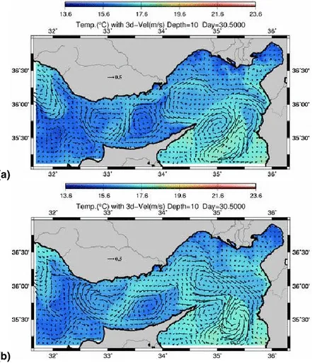
provided by the ETA model. Run D: Same as Run B except for penetrative radiation has been used. Temperatures at 10 m after a one month run with continuous forcing in January 2003, compared in Fig. 4 for the above cases, show differences between the tested cases, but at this point it is not possible to objectively assess which one should be better. The case A with non-interactive fluxes indicates much faster cooling

15

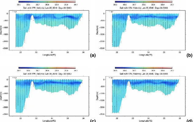
of surface waters as compared to the other cases. The interactive flux computations of case B and the flux computations using bulk formulae in case C do not seem to produce very different rates of cooling, but there are significant differences in the re-sulting surface circulation. The penetrative radiation case D results in much lower rates of cooling. Other comparisons between fields show significant changes especially up

20

to a depth of 100 m. The different mixing characteristics produced by the flux specifi-cations in cases A–D are compared in the salinity sections of Fig. 5. The low salinity modified Atlantic water present at mid-depths is used as a tracer to show differences in mixing, as they are influenced by the surface momentum, heat and salt fluxes. Fi-nally the comparison of surface fluxes for the above cases during the January 2003

25

period is provided in Fig. 6. It is evident that the fluxes of all interactive computation cases B, C, D are similar to each other, but very different from the non-interactive case A which uses constant surface salinity and surface variables provided from the atmo-spheric model. In particular, the salt flux for the non-interactive is not realistic because

(9)

OSD

3, 1481–1514, 2006

EGU of the constant surface salinity value assigned, and the heat fluxes are much higher

than the other cases. On the other hand, the flux computations using the bulk formulae in case C, produce slightly higher salt and lower heat fluxes from the sea surface to the atmosphere, in comparison to the atmospheric boundary layer formulation in cases B and D. The non-penetrative versus penetrative radiation formulation in cases B and

5

D of course do not affect the fluxes, but the latter results in lower rate of cooling as a result of the radiation heat source distributed near the surface waters.

3 Operational forecasts

An intensive data collection and assimilation effort was made during the 6 month Tar-get Operational Period beginning in September 2004, producing weekly forecasts of 5

10

days for the entire series of nested MFSTEP model domains. Examples of forecasts are provided here. In September–November 2004 period, the persistent anticyclonic eddy east of Cyprus (Figs. 2a, b) moved north (Fig. 7a) and created persistent jet flows (Fig. 7b) following the “tip” of Cyprus, impinging on the Gulf of ˙Iskenderun, and feeding the Asia Minor current flowing west along the northern continental slope. In

15

mid-November a sudden change in direction of surface currents due to wind and re-mote forcing (Fig. 7c) was followed by a temporary switch in currents in December and January to flow along the Syrian coast (Figs. 7d, e). The flow through the Cilician Basin was observed to have a significant barotropic component with current speeds reaching up to 0.3 m/s at 500 m depth. In June 2005 an upwelling event developed

simultane-20

ously south of Cyprus and along the Turkish coast in western Cilician Basin (Fig. 7f), which was well reproduced in the model (Fig. 7g). Shelf scale motions are displayed by focusing into specific regions. The meso-scale circulations developed in ˙Iskenderun Bay are exemplified in Fig. 7h. In this example, the flow along the shelf slope by-passes the Bay across its southwest opening, while a branch circulates cyclonically in

25

the Bay, as suggested earlier in Fig. 2c. Other types of circulation entering the bay on the surface with a return flow at deeper layers were also detected. However unsteady

(10)

OSD

3, 1481–1514, 2006

EGU effects resulting from weekly initialization cycles affected the results, and were recently

remedied by continuous forecasts that were implemented.

4 Evaluating extended forecasts

The performance of the model forecasts in active and slave mode, i.e. the model ini-tialized and running with continuously updated surface and lateral boundary conditions

5

compared with the model re-initialized at intervals was evaluated. For this purpose the January 2005 data were used to make forecasts for a full month with continuous updates versus the model re-initialized every week. The comparison of the circulations at the target date of 27 January 2005 for forecasts re-initialized at weekly intervals are given in Figs. 8 and 9 for depths of 10 m and 800 m respectively. At 10 m the forecasts

10

(Fig. 8) at the target date do not differ too much for the initializations done 3–4 weeks before the target date, but seem to deteriorate in features for initializations 1–2 weeks before the target date. At 800 m depth (Fig. 9), again we see the same result, indicat-ing that at least three-four weeks are needed for the deep features to develop, such as the eddies developed near the bottom as a result of the channel topography of the

15

Cilician Basin. The mean and standard deviations of fields generated from the weekly initializations are compared in Figs. 10 and 11 for depths of 10 m and 100 m respec-tively. It is clearly indicated that the weekly forecasts can not build up the kinetic energy compared to longer forecasts. The temperature and salinity fields show similar mean values but with very different details indicated by the standard deviations. The salinity

20

change appears the same as in the coarse model, while the temperature initial condi-tions from the coarse model at weekly intervals are different from those forecasted by the fine scale model because of different flux formulations and resolution.

(11)

OSD

3, 1481–1514, 2006

EGU

5 Conclusions

Experience and development achieved during the MFSTEP exercise give sufficient confidence for forecasting Cilician Basin circulation at high resolution shelf scales. The extension of the model domain to the entire northern Levantine coast and shelf regions along Asia Minor are under way.

5

Acknowledgements. This work was supported by the MFSTEP project (contract no

EVK-CT-2002-00075, 2003-2006) under FP5 of the Commission of the European Community, with N. Pinardi as the coordinator. We thank S¸ . Bes¸iktepe and the Institute of Marine Sciences of METU for support, and H. Örek for the satellite data processing. Related studies currently are being continued under the Cilician Basin (T ÜBITAK 105Y277) and MOMA (T ÜBITAK 105G029)

10

(12)

OSD

3, 1481–1514, 2006

EGU

References

Bignami, F., Marullo, S., Santoleri, R., and Schiano, M. E.: Longwave Radiation Budget in the Mediterranean Sea, J. Geophys. Res., 100(C2), 2501–2514, 1995.

Castellari, S., Pinardi, N., and Leaman, K.: A Model Study of Air-Sea Interactions in the Mediterranean Sea, J. Mar. Syst., 18, 89–114, 1998.

5

Collins, M. B. and Banner, F. T.: Secchi disk depths, suspensions and circulation in Northeast-ern Mediterranean Sea, Marine Geology, 31, M39–M46, 1979.

De Mey, P., Lascaratos, A., Manzella, G., and Pinardi, N. (Guest Editors): Mediterranean Fore-casting System Pilot Project – Parts I and II, Ann. Geophys. (Special Issue), 21, 436, 2003. Horton, C., Clifford, M., Schmitz, J., and Kantha, L. H.: A real-time oceanographic

now-10

cast/forecast system for the Mediterranean Sea, J. Geophys. Res., 102(C11), 25 123– 25 156, 1997.

Kondo, J.: Air-sea bulk transfer coefficients in diabatic conditions, Boundary-Layer Meteorol., 9, 91–112, 1975.

Korres, G. and Lascaratos, A.: A one-way nested eddy resolving model of the Aegean and

15

Levantine basins: Implementation and Climatological Runs, Ann. Geophys., 21, 205–220, 2003.

Launiainen, J. and Vihma, T.: Derivation of turbulent surface fluxes – an iterative flux-profile method allowing arbitrary observing heights, Environmental Software, 5(3), 113–124, 1990. ¨

Ozsoy, E.: On the Atmospheric Factors Affecting the Levantine Sea, European Center for

20

Medium Range Weather Forecasts, Reading, UK, Technical Report No. 25, 30p, 1981. ¨

Ozsoy, E., Hecht, A., Ünl üata, Ü., Brenner, S., Sur, H. ˙I., Bishop, J., Latif, M. A., Rozentraub, Z., and Ouz, T.: A Synthesis of the Levantine Basin Circulation and Hydrography, 1985–1990, Deep-Sea Res., 40, 1075–1119, 1993.

Pinardi, N., Arneri, E., Crise, A., Ravaioli, M., and Zavatarelli, M.: The physical, sedimentary

25

and ecological structure and variability of shelf areas in the Mediterranean Sea, The Sea, 14, 2005.

Reiter, E. R.: Handbook for Forecasters in the Mediterranean, Weather Phenomena of the Mediterranean Basin, Part 1: General Description of the Meteorological Processes, Tech. Pap. 5–75, 344 pp., Environmental Prediction Research Facility, Naval Postgraduate School,

30

Monterey, California, 1979.

(13)

OSD

3, 1481–1514, 2006

EGU

Oceanogr., 18(11), 1601–1626, 1988.

The POEM Group: Robinson, A. R., Malanotte-Rizzoli, P., Hecht, A., Michelato, A., Roether, W., Theocharis, A., Ünl üata, Ü., Pinardi, N., Artegiani, A., Bishop, J., Brenner, S., Chris-tianidis, S., Gacic, M., Georgopoulos, D., Golnaraghi, M., Hausmann, M., Junghaus, H.-G., Lascaratos, A., Latif, M. A., Leslie, W. G., O ˘guz, T., Özsoy, E., Papageorgiou, E., Paschini,

5

E., Rosentroub, Z., Sansone, E., Scarazzato, P., Schlitzer, R., Spezie, G.-C., Zodiatis, G., Athanassiadou, L., Gerges, M., and Osman, M.: General Circulation of the Eastern Mediter-ranean, Earth Sci. Rev., 32, 285–309, 1992.

Vihma, T.: Atmosphere-Surface Interactions over Polar Oceans and Heteregenous Surfaces, Finnish Marine Research, 264, 3–41, 1995.

(14)

OSD

3, 1481–1514, 2006

EGU

Table 1. Domain and grid characteristics of the Cilician Basin / Shelf Model n.m – dimensions

of grid, λ. φ – longitude and latitude coordinates. x. y – distance coordinates. n ∆λ (◦) ∆x (km) λ₁(◦) λ₂(◦) λ₂–λ₁(◦) x₂–x₁(km) 303 0.01500 1.35 31.700 36.245 4.545 408.6 m ∆φ (◦) ∆y (km) φ₁(◦) φ₂(◦) φ₂–φ₁(◦) y₂– y₁(km) 150 0.01206 1.35 35.120 36.929 1.809 201.1

(15)

OSD

3, 1481–1514, 2006

EGU

(16)

OSD

3, 1481–1514, 2006

EGU

(a) Fig. 2. (a) Eddies, jets and gyres in the Levantine Basin of the Eastern Mediterranean Sea

revealed in satellite-derived sea surface temperature field of 28 September 2004,(b) Cilician

Basin model 5 day forecast of 10 m currents and temperature on 27 September 2004, (c)

schematic surface circulation of Mersin Bay and the Gulf of ˙Iskenderun area (continuous line: summer, dashed line: winter) suggested by Collins and Banner (1979).

(17)

OSD

3, 1481–1514, 2006

EGU

(b) Fig. 2. Continued.

(18)

OSD

3, 1481–1514, 2006

EGU

(c) Fig. 2. Continued.

(19)

OSD

3, 1481–1514, 2006

EGU

(a) (b)

Fig. 3. Model bathymetry (depth in m) of (a) the fine grid Cilician Basin/Shelf Model, and (b) the

difference between coarse and fine grid bathymetry data sets with coarse grid data interpolated and the difference calculated on the fine grid.

(20)

OSD

3, 1481–1514, 2006

EGU

(a)

(b)

Fig. 4. (a) Currents and temperature at 10 m depth for run A, run B (b), run C (c), run D (d) on

(21)

OSD

3, 1481–1514, 2006

Printer-friendly Version Interactive Discussion EGU (c) (d) Fig. 4. Continued.

(22)

OSD

3, 1481–1514, 2006

EGU

(a) (b)

(c) (d)

Fig. 5. Comparison of salinity fields along the west-east section at 36◦N for(a) run A, (b) run

(23)

OSD

3, 1481–1514, 2006

EGU

Fig. 6. (a) Salt flux, (b) heat flux and (c) wind stress for runs A (solid line), B (dashed line), C

(24)

OSD

3, 1481–1514, 2006

EGU

(a) Fig. 7. (a) Satellite sst image on 11 November 2004, (b) forecast currents and temperature

at 10 m depth for a 5 day forecast on 8 November 2004, 12:00 UTC(c) same for 22

Novem-ber 2004 and(d) 6 December 2004, (e) sst image on 11 January 2005 (f) sst image on 17

June 2005, (g) currents and temperature at 10 m depth for 21 June 2005, (h) currents and

(25)

OSD

3, 1481–1514, 2006

EGU

(b) Fig. 7. Continued.

(26)

OSD

3, 1481–1514, 2006

EGU

(c) Fig. 7. Continued.

(27)

OSD

3, 1481–1514, 2006

EGU

(d) Fig. 7. Continued.

(28)

OSD

3, 1481–1514, 2006

EGU

(e) Fig. 7. Continued.

(29)

OSD

3, 1481–1514, 2006

EGU

(f) Fig. 7. Continued.

(30)

OSD

3, 1481–1514, 2006

EGU

(g) Fig. 7. Continued.

(31)

OSD

3, 1481–1514, 2006

EGU

(h) Fig. 7. Continued.

(32)

OSD

3, 1481–1514, 2006

EGU

Fig. 8. Comparison of forecasts at 10 m depth at the target date of 27 January 2005 for runs

initialized at different dates and run with continuously updated hourly atmospheric fluxes and daily lateral boundary conditions through January 2005. Initializations are on(a) 1 January, (b)

(33)

OSD

3, 1481–1514, 2006

EGU

Fig. 9. Comparison of forecasts at 800 m depth at the target date of 27 January 2005 for runs

initialized at different dates and run with continuously updated hourly atmospheric fluxes and daily lateral boundary conditions through January 2005. Initializations are on(a) 1 January, (b)

(34)

OSD

3, 1481–1514, 2006

EGU

Fig. 10. Comparison of runs initialized at different dates and run with continuously updated

hourly atmospheric fluxes and daily lateral boundary conditions through January 2005. Com-parison of field statistics averaged over the model domain at 10 m depth(a) mean salinity, (b)

standard deviation of salinity(c) mean temperature (d) standard deviation of temperature (e)

kinetic energy density. Initializations are on 1 January 2005 (solid line), 8 January, 15 January and 22 January (dashed lines) 2005.

(35)

OSD

3, 1481–1514, 2006

EGU

Fig. 11. Comparison of runs initialized at different dates and run with continuously updated

hourly atmospheric fluxes and daily lateral boundary conditions through January 2005. Com-parison of field statistics averaged over the model domain at 100 m depth(a) mean salinity, (b)

standard deviation of salinity(c) mean temperature (d) standard deviation of temperature (e)

kinetic energy density. Initializations are on 1 January 2005 (solid line), 8 January, 15 January, and 22 January (dashed lines) 2005.