Operational coastal ocean forecasting in the Eastern Mediterranean: implementation and evaluation

HAL Id: hal-00298386

https://hal.archives-ouvertes.fr/hal-00298386

HAL is a multi-disciplinary open access

archive for the deposit and dissemination of sci-entific research documents, whether they are pub-lished or not. The documents may come from teaching and research institutions in France or abroad, or from public or private research centers.

L’archive ouverte pluridisciplinaire HAL, est destinée au dépôt et à la diffusion de documents scientifiques de niveau recherche, publiés ou non, émanant des établissements d’enseignement et de recherche français ou étrangers, des laboratoires publics ou privés.

Operational coastal ocean forecasting in the Eastern

Mediterranean: implementation and evaluation

G. Zodiatis, R. Lardner, D. R. Hayes, G. Georgiou, S. Sofianos, N. Skliris, A.

Lascaratos

To cite this version:

G. Zodiatis, R. Lardner, D. R. Hayes, G. Georgiou, S. Sofianos, et al.. Operational coastal ocean forecasting in the Eastern Mediterranean: implementation and evaluation. Ocean Science Discussions, European Geosciences Union, 2006, 3 (3), pp.397-434. �hal-00298386�

OSD

Printer-friendly Version Interactive Discussion Ocean Sci. Discuss., 3, 397–434, 2006

www.ocean-sci-discuss.net/3/397/2006/ © Author(s) 2006. This work is licensed under a Creative Commons License.

Ocean Science Discussions

Papers published in Ocean Science Discussions are under open-access review for the journal Ocean Science

Operational coastal ocean forecasting in

the Eastern Mediterranean:

implementation and evaluation

G. Zodiatis1, R. Lardner1, D. R. Hayes1, G. Georgiou1, S. Sofianos2, N. Skliris2, and A. Lascaratos2

1

Oceanography Centre, University of Cyprus, P.O. Box 20537, 1678 Nicosia, Cyprus

2

Applied Physics Dept., Ocean Physics Modelling Group, University of Athens, Greece Received: 28 March 2006 – Accepted: 27 April 2006 – Published: 8 June 2006 Correspondence to: D. R. Hayes (dhayes@ucy.ac.cy)

OSD

Printer-friendly Version Interactive Discussion

Abstract

The Cyprus Coastal Ocean Forecasting and Observing System (CYCOFOS) has been producing operational flow forecasts of the northeastern Levantine Basin since 2002 and has been substantially improved in 2005. It is the first system in the Mediter-ranean to produce a forecast every day at the coastal scale. CYCOFOS uses a the 5

POM (Princeton Ocean Model) flow model, and recently, within the frame of the MF-STEP project (Mediterranean Forecasting System, Toward Environmental Prediction), the flow model was upgraded to use the hourly SKIRON atmospheric forcing, and its resolution was increased from 2.5 km to 1.8 km. The CYCOFOS model is now nested in the ALERMO (Aegean Levantine Eddy Resolving Model) regional model from the 10

University of Athens, which is nested within the MFS (Mediterranean Forecasting Sys-tem) basin model. The Variational Initialization and FOrcing Platform (VIFOP) has been implemented to reduce the numerical transient processes following initialization. Moreover, a five-day forecast is repeated every day, providing more detailed and more accurate information, of particular value to coastal end users. Forecast results are 15

posted on the web pagehttp://www.ucy.ac.cy/cyocean. The new, daily, high-resolution forecasts agree exceptionally well with the ALERMO regional model. The agreement is better and results more reasonable when VIFOP is used. Active and slave experiments suggest that a four-week active period produces realistic results with more small-scale features. Bias with respect to the slave mode is negligible and there is no detectable 20

bias with remote sensing images (for September, 2004). In situ observed hydrographic data from south of Cyprus are similar in many ways to the corresponding forecast fields. Plans for further model improvement include assimilation of observed temper-ature profiles (XBT), conductivity-tempertemper-atudepth (CTD) profiles from drifters or re-search cruises, and CT data from the CYCOFOS ocean observatory.

OSD

Printer-friendly Version Interactive Discussion

1 Introduction

Knowledge of seawater movements and properties is of importance in forecasting the effects of human activities on the marine environment as well as the effect of marine conditions on human operations in the sea. Today, flow modelling is considered a necessary operational tool, useful to aid decision-making in case of marine accidents. 5

Some examples where operational forecasting is vital include search and rescue, oil spill fate modelling, and dispersion of pollutants. The practical real-time benefits of operational oceanography also bring improved understanding of environmental condi-tions and change at many levels. These operational activities imply a close attention to marine conditions on a daily basis over a period of years and from basin scales down 10

to coastal scales. For these reasons, among others, the European Union has pro-moted several projects in order to implement operational oceanography. One of these projects is the Mediterranean Forecasting System (MFS) (Pinardi et al., 2003) which includes the implementation of advanced modelling and data assimilation tools for near real time prediction. The oceanographic prediction models are: 1. A basin model with 15

7 km resolution over the whole Mediterranean Sea. 2. Several Intermediate/Regional Models nested within the basin with 3 km resolution. 3. One or more coastal/shelf models nested within each regional model. The shelf models have a 1.8 km resolution. The Cyprus Coastal Ocean Model (CYCOM) is one of the coastal/shelf models of the MFS project, for high resolution flow simulations in the Cyprus and the NE Levantine 20

basins. It is nested within the Aegean Levantine Eddy Resolving Model (ALERMO), which covers the whole Eastern portion of the Mediterranean Sea. In this paper the performance of CYCOM is investigated by examining the effects of downscaling and initializing from the regional model and the degree of agreement with remote-sensing and in situ data.

25

OSD

Printer-friendly Version Interactive Discussion

2 Methods and model descriptions

Both CYCOM and ALERMO use numerical schemes that are modified versions of POM (the Princeton Ocean Model). The POM model has been widely used both within the framework of the MFS and elsewhere to simulate the flows in both regional and coastal/shelf sea areas of the Mediterranean Sea. POM has been extensively de-5

scribed in the literature (Blumberg and Mellor, 1987; Lascaratos and Nittis, 1998; Za-vatarelli and Mellor, 1995). The POM model is a primitive equation, 3-D ocean circula-tion model based on the full nonlinear equacircula-tions of momentum and mass conservacircula-tion and their depth averaged forms. The model comprises a bottom-following sigma coor-dinate system, a free surface, and split mode time steps. At each time-step, the sur-10

face elevation and vertically integrated mass transports (that is, the barotropic mode) are computed from the depth-averaged equations by an explicit leapfrog scheme. The vertical structure of the current (baroclinic mode) is obtained from the horizontal mo-mentum equations with a longer time step (Lardner and Cekirge, 1998). Advancing the baroclinic mode is computationally much more demanding and the use of a longer time 15

step for it makes the overall computational scheme quite efficient. All sub-grid-scale phenomena are considered as mixing processes by introducing separate horizontal and vertical mixing terms. The horizontal viscosity and diffusion terms are evaluated using the Smagorinsky (1963) horizontal diffusion formulation while the vertical mixing coefficients for momentum and tracers are computed according to the Mellor-Yamada 20

2.5 turbulence closure scheme (Mellor and Yamada, 1982). Heat and salinity transport sub-models are included. Potential temperature, salinity, velocity and surface elevation, are the prognostic variables of the model.

2.1 Cyprus Coastal Model (CYCOM)

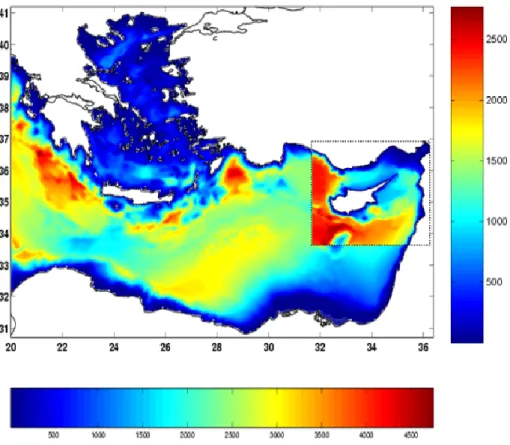
The domain of CYCOM (Fig. 1) is bounded by coastline on the north and east (max-25

imum latitude of 36◦550N and maximum longitude of 36◦130E). The open boundary to the south is the 33◦300N latitude line, and the open boundary to the west is the

OSD

Printer-friendly Version Interactive Discussion 31◦300E meridian. Horizontal Cartesian co-ordinates are in the Mercator projection

with an Arakawa C-grid, and the resolution is uniform at one minute (approximately 1.8 km) for a total of 284×206 horizontal grid points. The grid-spacing is sufficiently small to resolve steep bathymetry in the region as well as features with internal Rossby radius length scales (10–15 km). In the vertical, a non-uniform grid of 25 sigma layers 5

was used with exponentially decreasing spacing near the surface and sea bed to pro-vide finer resolution of the surface and bed layers. The bottom topography is based on the 10×10high resolution U.S. Navy Digital Bathymetric Database. The equations used in CYCOM are described in Zodiatis et al. (2003).

In order to initialize CYCOM, the ALERMO data are downscaled from its lower res-10

olution, larger domain using VIFOP (Variational Initialization and Forcing Optimization Platform). The Variational Initialization technique (Auclair et al., 2000a, b) analyses the outputs of the regional scale circulation model used as initial field of high resolution ocean models to reduce the amplitude of the numerical transient processes following the initialization. The VIFOP package was successfully implemented and configured in 15

the CYCOM model as in ALERMO, which had first used VIFOP for downscaling from the Mediterranean basin model. Previously, bilinear interpolation in the horizontal was used. (No interpolation is necessary in the vertical since the same sigma layers are used.) The procedure for nesting within ALERMO (resolution of 3 km) is identical to that described by Zodiatis et al. (2003). A passive, one way interaction is used (Spall 20

and Holland, 1991), where the nesting provides for information to be passed along the open boundaries from the ALERMO coarse grid to the CYCOM high-resolution grid model.

Surface and bottom boundary conditions are applied as described in Zodiatis et al. (2003). Surface boundary forcing is provided by the SKIRON 5-day forecast. The 25

high-resolution (0.1◦) and high-frequency (hourly) forecast is available daily. These daily atmospheric forecasts are used for each new ocean forecast using the bulk flux formulation. Downward shortwave and longwave radiation are used directly from SK-IRON, while heat loss terms are calculated from SKIRON-provided parameters.

OSD

Printer-friendly Version Interactive Discussion ble and latent heat are calculated from Budyko (1963), longwave loss is calculated from

Bignami (1995). Evaporation is also calculated from Budyko (1963) and combined with SKIRON-provided precipitation for surface salinity flux. Surface momentum fluxes are calculated using the computed drag coefficient of Hellerman and Rosenstein (1983). There is no relaxation of surface fluxes.

5

The daily average fields are posted on the web site: http://www.ucy.ac.cy/cyocean. Five subregions can be viewed online and forecast data can be downloaded for user-visualization using the Visual Interface of Oceanographic Data, VIOD, or for use in the oil spill model, MEDSLIK. Both of these programs are freely available. In addition, 6-hourly averages are also now available.

10

2.2 Aegean-Levantine Eddy Resolving Model (ALERMO)

The ALERMO model has been implemented, developed and tested within the frame-work of the Mediterranean Forecasting System activities, (Korres and Lascaratos, 2003) including application of the Variational Initialization method. ALERMO’s reso-lution has been increased from previous implementation to 1/30◦×1/30◦ and several 15

new numerical schemes have been implemented into the model in order to increase its forecasting efficiency.

The ALERMO model covers the geographical area 20◦E–36.4◦E, 30.7◦N–41.2◦N and has one open boundary located at 20◦E as shown in Fig. 1. The computational grid has a horizontal resolution of 1/30◦×1/30◦ (493×316 grid points) and 25 sigma 20

levels in vertical with a logarithmic distribution near the sea surface, which results in a better representation of the surface mixed layer.

The U.S. Navy Digital Bathymetric Data Base I (1/60◦×1/60◦) was used for building up model’s bathymetry using bilinear interpolation to map the data onto the model’s grid. The minimum depth in shallow areas has been set equal to 25 m. Seasonal 25

hydrological data necessary for the evaluation of the horizontal diffusion terms for trac-ers during the model integration were taken after proper bi-linear interpolation from the MODB-MED4 seasonal climatological data base (Brasseur et al., 1996). The upgraded

OSD

Printer-friendly Version Interactive Discussion ALERMO version uses a real freshwater flux boundary condition.

The one-way nesting with the global Mediterranean OGCM is applied along the west-ern boundary of ALERMO (located at 20◦E) and is thoroughly described in Korres and Lascaratos (2003). The nesting between the two models involves the zonal/meridional velocity components, temperature and salinity. The nesting scheme has been exten-5

sively tested during MFSPP under both climatological and high frequency atmospheric forcing. During TOP, daily averaged OGCM variables are linearly interpolated in time and mapped onto ALERMO’s open boundary section using bi-linear interpolation in the horizontal and linear interpolation along the vertical. Normal velocities at the open boundary are constrained so that the volume transport is conserved between ALERMO 10

and the OGCM.

The ETA atmospheric model used in the SKIRON system is an operational weather prediction model, currently running with a 1/10◦×1/10◦ horizontal resolution analysis (Kallos et al., 1997) for the needs of Mediterranean Forecasting System Toward En-vironmental Prediction (MFSTEP). It provides 10-m wind speed, 2-m air temperature 15

and relative humidity, the precipitation rate, the shortwave radiative gain by the ocean and the infrared atmospheric radiation reaching the sea surface. These atmospheric fluxes/parameters (linearly interpolated in time) are then used by the ALERMO model for the estimation of the heat, freshwater and momentum budget at the sea surface at each time step of the model’s integration. The coupling between the ALERMO and the 20

ETA model is designed in such a way to allow one-way feedback ocean-atmosphere mechanisms to take place. The oceanic model is free to adjust the evaporative, upward longwave radiation and sensible heat flux consistently with its own surface temperature using proper bulk formulae (Korres et al., 2002).

The ALERMO model is initialized from the MFSTEP OGCM (operationally on a 25

weakly basis during the TOP period) using the Variational Initialization (VI) method (Auclair et al., 2000a). The VIFOP (Variational Initialization and Forcing Optimization Platform) package including the tangent linear of the POM model, was successfully implemented and configured in the ALERMO model. The VI procedure is performed

OSD

Printer-friendly Version Interactive Discussion using only the external mode of the “background” field which is dynamically optimized

to reduce the amplitude of the spurious external gravity wave generations during the initialization process. The constraints for the variational initialisation of the external mode used in ALERMO are: 1) Optimization of the global divergence, 2) optimisation of the surface elevation tendency, and 3) optimisation of the surface elevation tendency 5

as a strong constraint. The extrapolation modulus has also been included.

The ALERMO forecasting system was initialized in 1 September 2004, producing 5-days forecast on a weekly basis. Currently the forecast is operated on daily basis with the configuration described above. A series of sensitivity experiments (very high resolution atmospheric forcing – 5 km, active vs. slave modes of forecasting, etc.) has 10

been performed as well as model validation, in order to evaluate the forecasting skill and perform tuning adjustments. Besides CYCOM, other high resolution (∼1.5 km) shelf operational models are nested in the ALERMO system.

2.3 Operational mode

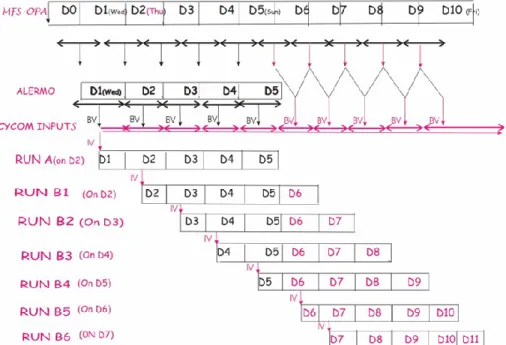
The method by which CYCOM is initialized and forced for operational forecasts is il-15

lustrated in Fig. 2. Every Thursday, CYCOM is initialized with the 24-h average fields centered at noon Thursday from the Wednesday ALERMO forecast (a 5-day forecast). Similarly, ALERMO is initialized every Wednesday from a 24-h average field centered at noon from the Tuesday MFS basin model (a 10-day forecast). Domains are illus-trated in Fig. 1. VIFOP is used to downscale both the MFS basin and the ALERMO, 20

as mentioned above. Forecasts run days other than Thursday are initialized with an in-stantaneous field from a previous CYCOM forecast, but with the updated atmospheric forecast. At the time of this study analysis, ALERMO was running weekly, so some of the daily CYCOM forecasts used MFS basin model lateral boundary conditions. Lateral boundary conditions were available from ALERMO on Wednesday through Sunday and 25

by MFS basin model on Monday and Tuesday. In this way, it was possible to compute 5-day forecasts every day.

OSD

Printer-friendly Version Interactive Discussion

3 Results

3.1 Model-model comparisons

3.1.1 Downscaling from regional to coastal models

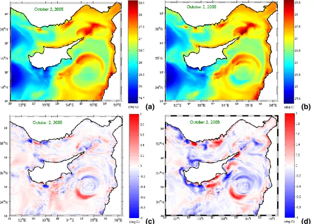
A forecast produced on 28 September 2005 is now discussed in detail in order to com-pare the results of two methods of downscaling: bilinear interpolation and Variational 5

Initialization (VI). Average CYCOM fields of sea surface temperature centered at noon of the fourth day of the forecast, 2 October 2005 are compared with the ALERMO forecast on the same day (fifth day for that forecast). Comparison is better when the bilinear interpolation method is replaced by the VIFOP method of downscaling. The surface temperature field produced by ALERMO (Fig. 3a) and CYCOM using the VI-10

FOP method (Fig. 3b) differ in small areas near the coast (Fig. 3c). In these regions, the models differ by a few tenths of a degree Celsius up to 1◦C for a very small number of grid points. Over the whole domain, the mean difference is −0.0020◦C (CYCOM slightly warmer), and the standard deviation is 0.154◦C. When only bilinear interpola-tion is used, CYCOM differs much more from ALERMO in the regions near to the coast 15

of Cyprus (Fig. 3d). In this case, the mean temperature difference is −0.0357◦C and standard deviation is 0.238◦C. Similar differences are seen in surface velocity. Using VIFOP improves flow direction and strength in many cases. (Flow into the coast is less common.) The use of VIFOP reduces errors caused by the generation of surface grav-ity waves when an interpolated velocgrav-ity interacts with high-resolution coastal features 20

not present in the lower resolution model. 3.1.2 Slave-active comparisons

As discussed in the accompanying paper of Sarantis et al. (2006), experiments have been performed in order to investigate the effect of initialization of a model nested within a coarser resolution model. As in the operational mode, in the “slave” mode, 25

OSD

Printer-friendly Version Interactive Discussion the high resolution model, CYCOM, is initialized every week from the coarse resolution

model (ALERMO). The dynamical features that develop over this period are compared to those of an experiment with the same boundary and initial conditions, but with four weeks of integration without initialization (“active” mode). These experiments have been performed at the regional scale: ALERMO was run in both modes using the MFS 5

basin model for initialization and boundary conditions and SKIRON best analysis data for surface forcing. At the coastal scale, CYCOM has been run in both “active” and “slave” modes using the ALERMO output.

In the first experiment we will discuss, CYCOM simulated the month of January 2005 using the slave and active modes. To compare the results with those of the parent 10

model, several descriptive statistics have been computed. First, ALERMO output fields are bilinearly interpolated to the CYCOM grid, then the difference field is produced (ALERMO minus CYCOM). The difference field then is analyzed for its mean and stan-dard deviation to quantify the level of bias and variability between the two models. Every day of the output, a mean and standard deviation are computed. The evolu-15

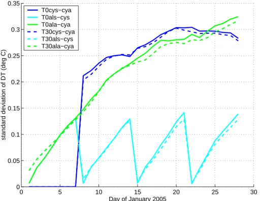
tion of the standard deviation in the surface temperature difference field indicates that the active run’s variability increases relative to the ALERMO active run over the four weeks, especially in the first two weeks (Fig. 4). In the operational mode of running, the ALERMO and CYCOM systems are both run in slave mode, and the variability in surface temperature increases each day until dropping back to zero on re-initialization 20

(Fig. 4). The last curve in Fig. 4 illustrates the level of variability between the CYCOM slave and CYCOM active, and it is shown that they differ more from each other than do the two active model runs. Of course during the first week, the two CYCOM runs are identical. The same pattern is present for surface salinity and velocity components at 0 m and 30 m, with 30 m variability slightly lower than 0 m (not shown).

25

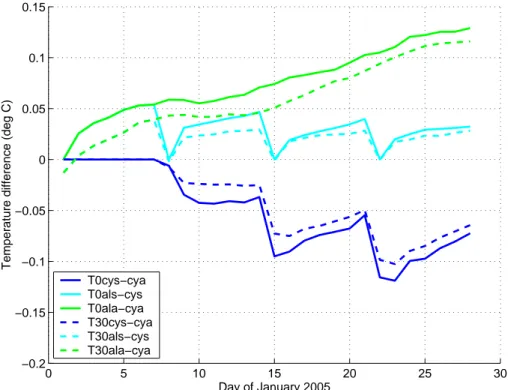
The mean bias between the two active runs (Fig. 5) indicates that the temperature fields near the surface are diverging: ALERMO is warming relative to CYCOM (or CYCOM is cooling relative to ALERMO). The bias is greater at the surface than at 30 m. The temperature fields of the CYCOM slave run compared to the ALERMO slave run at

OSD

Printer-friendly Version Interactive Discussion 0 m and 30 m, show the same divergence, but of course both are reinitialized before the

bias exceeds 0.05◦C. More complicated is the mean temperature difference between CYCOM slave and CYCOM active. It appears that aside from the relative warming of slave during the week-long active period (as above) the reinitialization of the slave causes a large relative cooling, which dominates the overall trend. The bias in salinity 5

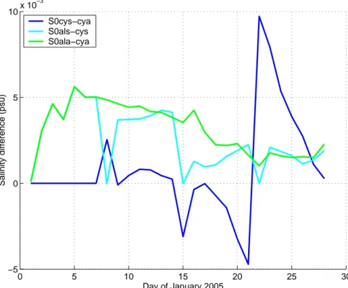
does not show a consistent trend (Fig. 6), in fact, the bias tends toward zero, except for the salinity difference between the CYCOM slave and CYCOM active. Apparently, the initialization of the slave from the coarse model on 21 January caused a large change in salinity not present in the active run. The bias in the velocity components is small and shows no trend for any case (not shown).

10

3.2 Model-observations comparison 3.2.1 Active-slave and remote sensing

The active CYCOM run from January, 2005, is now compared to remotely-observed sea surface temperature. Images of SST of the Levantine Basin are collected by the University of Cyprus Oceanography Centre’s HRPT ground receiving station for the 15

NOAA-AVHRR satellite system. Images have a spatial resolution of about 1 km. A SmarTrack software for stand-alone data reception is used, while for the processing of the raw IR data an integrated software package specifically developed by the CY-COFOS collaborators is in use for auto mode rectification (geometric correction) of the images and the computations of the SST. The computation of the SST is based on the 20

algorithms recommended by NOAA, using IR channels 4 and 5. The system is set up to receive data only from night or early morning satellites passages in order to avoid the hot spots that usually appear during daily SST images of the Levantine Basin most of the year.

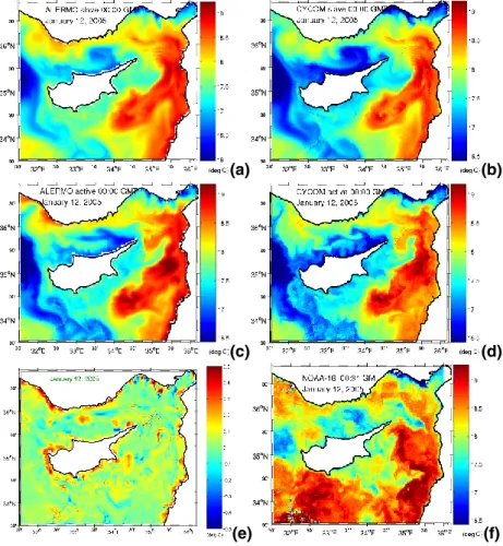
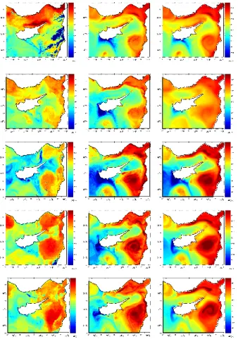
An SST image collected on 12 January 2005, 00:30 UT is compared with the active 25

and slave runs for January 2005 in Fig. 7. The SST of the two ALERMO runs (slave and active) are shown on the left column, and the two CYCOM runs on the right hand

OSD

Printer-friendly Version Interactive Discussion side. Firstly, all model runs have a similar structure and temperature range, with

vary-ing degrees of small-scale variability in the form of fronts and instabilities. Secondly, it is clear that the two active runs have more small scale structure than their correspond-ing slave runs, and the two CYCOM runs (6-hourly averages), becorrespond-ing at higher reso-lution and using shorter temporal average, have more small scale structure than the 5

ALERMO runs (24-h averages). Note that all panels use the same temperature scale. The spatial nature of the differences between active-active and active-slave model runs consists of fairly large-sized patches of error of the order of ±0.5◦C (not shown). How-ever, the temperature difference field of ALERMO slave minus CYCOM slave (Fig. 7e) contains similarly-sized errors in a narrow zone adjacent to all coastlines. The interior 10

differences are much less. The same behavior is seen in 30 m temperature, but no cor-responding zone exists for surface salinity or velocity at surface or 30 m. It is likely that the reinitialization introduces this difference, which is “forgotten” by the system after a sufficient time of “active” simulation time.

The remotely-sensed image (Fig. 7f), essentially instantaneous, has many similari-15

ties with the large scale structure of the model runs: a cool pool west of Cyprus (the edge of the Rhodes Gyre), a warm northward current along the Syrian coast which seems to continue into the northern Cilician basin as the Asia Minor current, relatively warm anticyclonic eddy east of Cyprus (slightly different locations). However, the mod-els indicate a cool current SW of Cyprus (entering the domain at 34◦ to 35◦N and 20

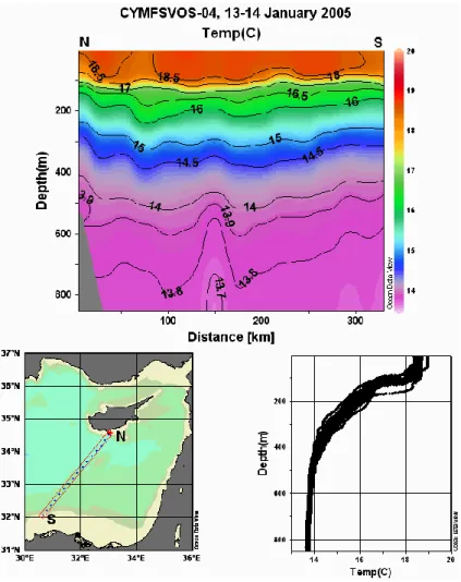
exiting at 32.5◦to 34◦E), whereas the NOAA image shows a large patch of warm water in this region, not a branch of cool water from the Rhodes Gyre. An XBT transect from this period shows a slightly cooler surface SW of Cyprus, although not of the degree or extent seen in the model (Fig. 8). In the XBT transect, there is a change from 18.8 to 18.4◦ covering a distance of about 20 km in the region, which is not clear in the NOAA 25

image and is less than the change in temperature seen in the model field in this region. Other SST images during January (of which there are few clear sky images) are similar to the one shown here. Both XBT and SST data were used by the MFS basin model for assimilation, and the analyses fields of the basin model (not shown) indicate a

re-OSD

Printer-friendly Version Interactive Discussion duction in the strength of the cool current relative to the forecast; however, it appears

the assimilation was not capable of changing the model state sufficiently in this region. In contrast, the active CYCOM run of September, 2004 agrees qualitatively with the remotely-sensed SST images available (Fig. 9). 3, 8, 14, 20, and 28 September are each represented by a row of images; the first image is the remotely-sensed SST from 5

the NOAA AVHRR system. The second column is the active CYCOM 6-hourly average closest to the time of the satellite observation. Also shown are the corresponding 24-h average ALERMO slave fields. The main features of the observed fields are present in the forecast fields: a large anticyclone southeast of Cyprus, warm water along the eastern and northern coasts of the Levantine, cooler waters around the coast of Cyprus 10

and in a region on the south coast of Turkey. The forecasts differ from the observations in that they suggest a persistent presence of cool water (likely to be upwelling) on the west and south of Cyprus. ALERMO and CYCOM agree except for the coastal regions south and east of Cyprus where ALERMO indicates significant temperature anomalies compared to the remotely-sensed images. In these regions, the CYCOM 15

agreement with the remotely-sensed images is excellent. While the CYCOM active run appears to contain smaller scale features than the coarse model and therefore be more realistic, it is informative to calculate the bias and root-mean-square differences between the observations and each model. See Table 1. The rms differences are nearly the same for both models, while the mean bias is inconsistent. For three of the 20

five days, ALERMO mean is closer to observations, while for the other two CYCOM active is closer. It is difficult to conclude quantitatively, then, that one model is “better” than the other. It is notable that the active run does not show a relative trend in mean surface temperature.

3.2.2 Active run and in situ data, August–September 2004 25

Intensive annual or semi-annual hydrographic cruises south of Cyprus have been car-ried out since 1995, and they enable model validation at a high level of detail. The cruises are part of the Cyprus Basin Oceanography (CYBO) program of the

OSD

Printer-friendly Version Interactive Discussion raphy Centre. Data are collected with an SBE 911+ system, which is calibrated on

an annual basis. Downcast data were processed first by manual removal of the initial thermal adjustment period and spikes. Next pressure, temperature, and salinity were low-pass filtered with time constants of 0.15, 0.5, and 1.0 s, respectively. The data dis-cussed here were collected during the period of 16–25 August 2004, (cruise CYBO-18) 5

a few weeks before the simulated period of September 2004. The 7th day of the active forecast will be presented here.

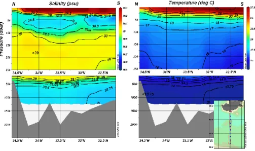
In this section of the paper, two vertical sections compare well to the September 2004 active experiment. Also, the simulated sea surface elevation is similar to the dy-namic height relative to 700 m calculated from CYBO-18 data. The north-south vertical 10

section of in situ measurements along 33◦E (Fig. 10) indicates clearly the warm, salty summertime mixed layer down to 30 m, the influence of Atlantic Water (AW) from 30 m down to 100 m, the Levantine Intermediate Water (LIW) from 100 m to 500 m, and the Eastern Mediterranean Deep Water (EMDW) below 500 m. The low salinity (<38.9 psu) AW is known to traverse the Levantine basin in the form of a meandering jet: the Mid-15

Mediterranean Jet (MMJ) (Zodiatis et al., 2005). The corresponding geostrophic veloc-ity perpendicular to the section presents a strong reversal in flow direction: eastward velocity north of 33.5◦N and westward velocity south of this location (Fig. 10c). The active forecast from 7 September 2004, shows the same overall situation, although the model domain extends no farther south than 33.5◦N (Fig. 11). Absolute values of 20

temperature and salinity are close to observations; at any given depth forecast tem-perature is generally within 1◦C of observations, and forecast salinity is within 0.1 psu of observations. Note that the same color scales are used throughout. The high salin-ity and temperature surface layer is present, but slightly less sharply defined. Atlantic Water is evident, as is LIW. The model predicted the same geostrophic velocity dipole, 25

but shifted to 33.75◦N (Fig. 11c).

The east-west section of observations along 34.5◦N shows stronger evidence of the AW, outside of the range 33–34◦E (Fig. 12a). Inside that range, where the bathymetry is relatively shallow, the AW signal is weak, and the surface layer is very thin. The

OSD

Printer-friendly Version Interactive Discussion active forecast agrees very well with the CYBO-18 east-west section: AW is present in

the west (although it extends only to 32◦E, not to 33◦E), the surface layer is thin in the region of shallow bathymetry, and the surface layer thickens towards the eastern edge of the section (Fig. 13). The intermediate depths are approximately 0.1 psu fresher in the forecast, and there is generally more horizontal variability visible in the forecast due 5

to the much higher horizontal resolution.

The dynamic height relative to 700 m for CYBO-18 presents strong evidence for the presence of a barotropic jet south of Cyprus (Fig. 14a). The jet enters the domain from the south, between 32◦E and 33◦E, makes an anticyclonic loop and exits the domain. The jet appears to bifurcate near 33.75◦N and 34◦E, with some flow southward out of 10

the domain and some northward along the edge of another anticyclonic feature visible at the eastern edge of the domain. A weaker current enters the western edge of the domain around 34.5◦N, bifurcates west of Cyprus, and the southern branch joins the current system discussed above. The CYCOM active forecast for 7 September 2004 contains two regions of elevated sea surface height in the same locations as the regions 15

of observed raised dynamic height, indicating similar anticyclonic features (Fig. 14b). The feature southeast of Cyprus is more intense in the forecast, however only the apparent edge of the feature is sampled during CYBO-18. Both diagrams imply the same strength and position of the barotropic current. Note the contour intervals are nearly the same (0.025 m for dynamic height and 0.02 m for sea surface elevation), as 20

are the full scale ranges (0.175 m and 0.20 m). 3.2.3 Slave run and in situ data, September 2005

Hydrographic data from CYBO-19 (9 to 19 September 2005) are now compared with the fourth day of the operational CYCOM forecast initialized on 9 September, 2005. The 24-h average fields for the fourth day of the forecast were used in order to allow 25

development of features not in the coarse model and because this day is near the mid-point of the cruise. The hydrographic data for the north-south section along the 33◦E meridian again indicate the influence of Atlantic Water from 34.0 to 34.4◦N, and at

OSD

Printer-friendly Version Interactive Discussion depths between 30 m and 90 m (Fig. 15a). The AW signal is weaker than observed in

2004. The summertime surface layer (slightly deeper than in 2004), LIW, and EMDW are all present. As in 2004, the thermocline deepens and warms from north to south (Fig. 15b). Much like CYBO-18, a dipole in zonal geostrophic velocity relative to 700 m is centred at 33.6◦N and extends from the surface down to 300 m (Fig. 15c). Com-5

pared to the observations, the model forecast section from the 13 September daily average contains a weaker and deeper low salinity core in the northern part (Fig. 16a). Differences in the sharpness of the thermocline and halocline are evident, the forecast indicating weaker stratification, as in the previous section. Also, the surface layer deep-ens in the model from north to south, but not in the observations (for the region in the 10

model domain: north of 33.5◦N). As in 2004, the LIW is slightly fresher in the model. The geostrophic velocity section does not indicate a dipole, but a similar eastward flow north of 33.5◦N. It should be noted once again that the model domain does not extend south of this point, where the westward geostrophic flow was indicated by CYBO-19 observations. The east-west sections for both CYBO-19 and the forecast (not shown) 15

are nearly identical to that of Figs. 12 and 13 except that for both the AW signal is weaker and in a slightly different position, and the surface layer was deeper.

Dynamic topography from observations and sea surface height from the forecast (Fig. 17) for September 2005 again suggest an anticyclonic circulation south of Cyprus. However, this time the region is much larger and the implied geostrophic zonal current 20

weaker. The location of the anticyclone in the model is slightly south and west of the observed location. Both forecast and observations show the edge of a cyclonic region west of Cyprus and regions of low sea surface height around the south coast. The major difference between the two is near the eastern edge of the domain where the model indicates increasing sea surface height (a secondary anticyclone) while the 25

OSD

Printer-friendly Version Interactive Discussion

4 Conclusions

A coastal flow forecasting system for the waters surrounding Cyprus and the Levantine basin is fully operational and producing good results. Through the internet, it provides forecasts of ocean flow, temperature, and salinity (daily and 6-hourly average fields are computed for the coming five days, every day). The Cyprus coastal flow model, 5

CYCOM, is initialized from the regional ALERMO model, using a variational initializa-tion method (VIFOP). In this configurainitializa-tion, the daily CYCOM forecast is shown to be in especially good agreement with the regional forecast on large scales, with most dif-ferences being small, near the coast, and/or beyond the resolution of ALERMO. Twin 28-day numerical experiments have been carried out where in one CYCOM is initial-10

ized every week from the coarse model (slave), and in the other initialized only at the beginning (active). The same has been done for ALERMO. Results indicate that the root-mean-square difference between the active and slave modes for CYCOM (near the surface for all variables) increases quickly in the first 14 days, but then grows slowly. The mean values of near-surface variables of each of the two modes show negligible 15

divergence, except for temperature (maximum 1.0◦C after 28 days). Simulated and remotely-sensed sea surface temperature show a qualitatively better agreement for the active runs due to the finer scale structures present (and illustrate the need for improved data assimilation in some regions and seasons). Neither active nor slave model temperatures drift significantly from the remote sensing observations. We feel 20

that the operational results of the forecasting system would benefit from a longer “ac-tive” period, perhaps two weeks instead of one. The potential drawback of unrealistic model fields appears to be insignificant, and the simulated (and realistic) increase in small-scale features is desired. Another benefit of longer active run simulations is the decrease in systematic differences in temperature near the coast, seen in slave-slave 25

comparisons even five days after initialization. Excellent agreement is found between forecasts (both active and operational) and in situ hydrographic data for 2004 and 2005. Both forecast and observations show the presence of relatively fresh Atlantic Water,

OSD

Printer-friendly Version Interactive Discussion plus the other characteristic water masses of the region. Geostrophic calculations for

both numerical and observational data show generally eastward flowing near-surface currents encircling an anticyclone south of Cyprus and cyclonic circulations west and southeast of Cyprus, in agreement with previous field studies (Zodiatis et al., 2004, 2005) and climatological numerical studies (Zodiatis et al., 2003).

5

CYCOM will be developed further by implementing assimilation of local observa-tions such as expendable bathythermographs (XBTs), conductivity-temperature-depth (CTD) profiles from drifters or hydrographic cruises, and CT data from the CYCOFOS ocean observatory. Sea level anomaly can also be assimilated when satellite altimeter tracks are available in our region.

10

Acknowledgements. This research has been carried out in the framework of the European

Union project MFSTEP, contract EVK3-CT-2002-00075. We acknowledge the support of the CYCOFOS collaborators: E. Demirov, D. Soloviev, S. Savva, M. Papaioannou, and T. Elefthe-riou. Figures 8, 10–17 have been whole or partially generated with Ocean Data View software (Schlitzer, 2006).

15

References

Auclair, F., Casitas, S., and Marsaleix, P.: Application of an inverse method to coastal modelling, J. Atmos. Oceanic Tech., 17, 1368–1391, 2000a.

Auclair, F., Marsaleix, P., and Estournel, C.: Truncation errors in coastal modelling: evaluation and reduction by an inverse method, J. Atmos. Oceanic Tech., 17, 1348–1367, 2000b.

20

Bignami, F., Marullo, S., Santoreli, R., and Schiano, M. A.: Longwave radiation budget in the Mediterranean sea, J. Geophys. Res., 100(c2): 2501–2514, 1995.

Blumberg, A. F. and Mellor, G. L.: A description of a three-dimensional coastal ocean circulation model, in: Three-Dimensional Coastal Ocean Circulation Models, Coastal Estuarine Sci., vol. 4, edited by: Heaps, N. S., AGU, Washington, D.C., 1–16, 1987.

25

Brasseur, P., Beckers, J. M., Brankart, J. M., and Schoenauen, R.: Seasonal temperature and salinity in the Mediterranean Sea: climatological analysis of a historical data set, Deep-Sea Res., 43, 159–192, 1996.

OSD

Printer-friendly Version Interactive Discussion

Budyko, M. I.: Atlas of the heat balance of the earth, Academic Press, San Diego, CA., 1963. Hellerman, S. and Rosenstein, M.: Normal wind stress over the world ocean with error

esti-mates, J. Phys. Ocean., 13, 1093–1104, 1983.

Kallos, G., Nickovic, S., Papadopoulos, A., Jovic, D., Kakaliagou, O., Misirlis, N., Boukas, L., Mimikou, N., Sakellaridis, G., Papageorgiou, J., Anadranistakis, E., and Manousakis, M.: The

5

regional weather forecasting system Skiron: An overview, Proceedings of the Symposium on Regional Weather Prediction on Parallel Computer Environments, 109–122, 15–17 October 1997, Athens, Greece, 1997.

Korres, G. and Lascaratos, A.: A one-way nested eddy resolving model of the Aegean and Levantine basins: implementation and climatological runs, Ann. Geophys., 21, 205–220,

10

2003.

Korres, G., Lascaratos, A., Hatziapostolou, E., and Katsafados, P.: Towards an ocean forecast-ing system for the Aegean Sea, Global Atmos. Ocean Syst., 8, 191–218, 2002.

Lardner, R. W. and Cekirge, H. M.: A new algorithm for three-dimensional tidal and storm surge computations, App. Math Model, 12, 471–571, 1988.

15

Lascaratos, A. and Nittis, K.: A high resolution three-dimensional numerical study of intermedi-ate wintermedi-ater formation in the Levantine Sea, J. Geophys. Res., 103(C9), 18 497–18 511, 1998. Mellor, G. and Yamada, T.: Development of a turbulent closure model for geophysical fluid

problems, Rev. Geophys., 20, 851–875, 1982.

Pinardi, N., Allen, I., Demirov, E., De Mey, P., Korres, G., Lascaratos, A., Le Traon, P. Y.,

20

Maillard, C., Manzella, G., and Tziavos, C.: The Mediterranean ocean forecasting system: first phase of implementation (1998–2001), Ann. Geophys., 21, 3–20, 2003.

Schlitzer, R.: Ocean Data View,http://odv.awi.de, 2006.

Smagorinsky, J.: General circulation experiments with the primitive equations. Part I: the basic experiment, Monthly Weath. Rev., 91, 99–165, 1963.

25

Spall, M. A. and Holland, W. R.: A nested primitive equation model for oceanic applications, J. Phys. Oceanogr., 21, 205–220, 1991.

Zavatarelli, M. and Mellor, G.: A numerical study of the Mediterranean sea circulation, J. Phys. Oceanogr., 25(6), 1384–1414, 1995.

Zodiatis, G., Drakopoulos, P., Brenner, S., and Groom, S.: Variability of the Cyprus warm core

30

eddy during the CYCLOPS project, Deep Sea Res. II, 52, 2897–2910, 2005.

Zodiatis, G., Lardner, R., Lascaratos, A., Georgiou, G., Korres, G., and Syrimis, M.: High resolution nested model for the Cyprus, NE Levantine basin, eastern Mediterranean Sea:

OSD

Printer-friendly Version Interactive Discussion

implementation and climatological runs, Ann. Geophys., 21, 221–236, 2003.

Zodiatis, G., Drakopoulos, P., and Gertman, I.: Modified Atlantic Water in the Levantine Basin, 37th CIESM Congress Proceedings, 37. Barcelona, Spain, 2004.

OSD

Printer-friendly Version Interactive Discussion Table 1. Mean and standard deviation of difference between remotely-sensed sea surface

temperature (T_REM) and either CYCOM active forecast (T_CY) or ALERMO slave forecast (T_AL). Five dates in September were analyzed (see Fig. 9 for temperature fields).

Day of T_REM-T_CY T_REM-T_AL Sep. 2005 (◦C) (◦C) STD MEAN STD MEAN 3 1.7 0.38 1.8 0.64 8 0.44 0.60 0.75 1.3 14 0.96 –0.57 1.0 –0.35 20 0.89 –0.11 0.95 0.20 28 0.59 –0.30 0.64 –0.53 417

OSD

Printer-friendly Version Interactive Discussion Fig. 1. Bathymetry and domain of ALERMO (color scale in meters along the bottom) and

OSD

Printer-friendly Version Interactive Discussion Fig. 2. Schema for operational mode of forecasting with CYCOM. Application of boundary

values are indicated by “BV” and initial conditions by “IV.”

OSD

Printer-friendly Version Interactive Discussion

(a) (b)

(c) (d)

Fig. 3. Sea surface temperature for operational mode forecasts from (a) ALERMO (b) CYCOM,

using the VIFOP method of initialization.(c) The temperature difference field of (a) and (b). (d).

The same as (c) but using the CYCOM forecast that did not use VIFOP. The output fields are 24-h averages on 2 October 2005, which was the fourth day of the forecast.

OSD

Printer-friendly Version Interactive Discussion 0 5 10 15 20 25 30 0 0.05 0.1 0.15 0.2 0.25 0.3 0.35 Day of January 2005

standard deviation of DT (deg C)

T0cys−cya T0als−cys T0ala−cya T30cys−cya T30als−cys T30ala−cya

Fig. 4. Root-mean-square differences of temperature between various runs throughout the

January 2005 experiment. Solid lines are for surface temperature, dotted are for 30 m. Blue line is for CYCOM slave minus CYCOM active. Cyan line is for ALERMO slave minus CYCOM slave. Green line is for ALERMO active minus CYCOM active.

OSD

Printer-friendly Version Interactive Discussion 0 5 10 15 20 25 30 −0.2 −0.15 −0.1 −0.05 0 0.05 0.1 0.15 Day of January 2005

Temperature difference (deg C)

T0cys−cya T0als−cys T0ala−cya T30cys−cya T30als−cys T30ala−cya

OSD

Printer-friendly Version Interactive Discussion 0 5 10 15 20 25 30 −5 0 5 10x 10 −3

Salinity difference (psu)

Day of January 2005 S0cys−cya

S0als−cys S0ala−cya

Fig. 6. Same as Fig. 5 but for salinity.

OSD

Printer-friendly Version Interactive Discussion

(a) (b)

(c) (d)

(e) (f)

Fig. 7. Sea surface temperature comparison for day 12 of active-slave experiment. (a)

ALERMO slave. (b) CYCOM slave. (c) ALERMO active. (d) CYCOM active. (e) Difference

between ALERMO slave and CYCOM slave. (f) Remotely-sensed image for the same day.

OSD

Printer-friendly Version Interactive Discussion Fig. 8. Expendable bathythermograph section from 13–14 January 2005.

OSD

Printer-friendly Version Interactive Discussion Fig. 9. SST comparison between remote-sensing, CYCOM active, ALERMO slave (from left

to right). Dates are from top to bottom: 3, 8, 14, 20, and 28 September 2004. No correction of observed images for clouds has been made (present in 3 September image). Temperature scales for ALERMO and CYCOM are the same. All plots on 14, 20, 28 September use a color scale of 23.5–28.5◦C. Plots on 3 and 8 September use a scale of 25–30◦C for model and

OSD

Printer-friendly Version Interactive Discussion Fig. 10. (a) and (b) Hydrographic section along 33◦E collected during CYBO-18 (16–25 August

2004).(c) Zonal geostrophic velocity relative to 700 m.

OSD

Printer-friendly Version Interactive Discussion Fig. 11. Same section as Fig. 10, but from 7 September 2004 active CYCOM forecast. Note

OSD

Printer-friendly Version Interactive Discussion Fig. 12. Hydrographic section along 34.5◦N collected during CYBO-18.

OSD

Printer-friendly Version Interactive Discussion Fig. 13. Same section as Fig. 12, but from 7 September 2004 active CYCOM forecast.

OSD

Printer-friendly Version Interactive Discussion (a)

(b)

Fig. 14. (a) Dynamic height at surface relative to 700 m for CYBO-18. (b) Surface elevation of

7 September 2004 active CYCOM run.

OSD

Printer-friendly Version Interactive Discussion Fig. 15. Same section as in Fig. 10, but for CYBO-19 (9 to 19 September 2005).

OSD

Printer-friendly Version Interactive Discussion Fig. 16. Same section as Fig. 10, but from 9 September 2005 operational CYCOM forecast

(day four of that forecast).

OSD

Printer-friendly Version Interactive Discussion (a)

(b)

Fig. 17. (a) Dynamic height at surface relative to 700 m for CYBO-19. (b) Surface elevation of