Evolution of tropospheric ozone under anthropogenic activities and associated radiative forcing of climate

HAL Id: hal-03124819

https://hal.archives-ouvertes.fr/hal-03124819

Submitted on 1 Feb 2021

HAL is a multi-disciplinary open access

archive for the deposit and dissemination of

sci-entific research documents, whether they are

pub-lished or not. The documents may come from

teaching and research institutions in France or

abroad, or from public or private research centers.

L’archive ouverte pluridisciplinaire HAL, est

destinée au dépôt et à la diffusion de documents

scientifiques de niveau recherche, publiés ou non,

émanant des établissements d’enseignement et de

recherche français ou étrangers, des laboratoires

publics ou privés.

Evolution of tropospheric ozone under anthropogenic

activities and associated radiative forcing of climate

D. Hauglustaine, G. Brasseur

To cite this version:

D. Hauglustaine, G. Brasseur. Evolution of tropospheric ozone under anthropogenic activities and

associated radiative forcing of climate. Journal of Geophysical Research: Atmospheres, American

Geophysical Union, 2001, 106 (D23), pp.32337-32360. �10.1029/2001JD900175�. �hal-03124819�

JOURNAL OF GEOPHYSICAL RESEARCH, VOL. 106, NO. D23, PAGES 32,337-32,360, DECEMBER 16, 2001

Evolution of tropospheric ozone under anthropogenic

activities and associated radiative forcing of climate

D. A. Hauglustaine

•

Service d'A6ronomie du CNRS, Paris, France

G. P. Brasseur 2

Max Planck Institute for Meteorology, Hamburg, Germany

Abstract. The budget of ozone and its evolution associated with anthropogenic

activities are simulated with the Model for Ozone and Related Chemical Tracers

(MOZART) '(version 1). We present the changes

in tropospheric

ozone and its

precursors

(CH4, NMHCs, CO, NOs) since the preindustrial period. The ozone

change at the surface exhibits a maximum increase at midlatitudes in the northern hemisphere reaching more than a factor of 3 over Europe, North America, and Southeast Asia during summer. The calculated preindustrial ozone levels are particularly sensitive to assumptions about natural and biomass burning emissions of precursors. The possible future evolution of ozone to the year 2050 is also simulated, using the Intergovernmental Panel on Climate Change IS92a scenario to estimate the global and geographical changes in surface emissions. The future evolution of ozone stresses the important role played by the tropics and the subtropics. In this case a maximum ozone increase is calculated in the northern subtropical region and is associated with increased emissions in Southeast Asia and Central America. The ozone future evolution also affects the more remote regions of

the troposphere,

and an increase

of 10-20% in background

ozone levels is calculated

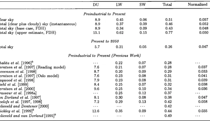
over marine regions in the southern hemisphere. Our best estimate of the global and annual mean radiative forcing associated with tropospheric ozone increase since

the preindustrial

era is 0.43 W m -•. This value

represents

about 207"•

of the forcing

associated with well-mixed greenhouse gases. The normalized tropospheric ozone

radiative

forcing

is 0.048 W m -• DU -1. An upper estimate

on our forcing

of 0.77

W m -2 is calculated

when a stratospheric

tracer is used

to approximate

background

ozone levels. In 2050 an additional ozone forcing of 0.26 W m -• is calculated,

providing

a forcing from preindustrial

to 2050 of 0.69 W m -•.

1. Introduction

A comparison between ozone measurements made during the nineteenth century and those made in re- cent decades suggests that concentrations have been in- creasing in the troposphere since preindustrial times. This change is attibuted to growing emissions of pre- cursors such as methane (CH4), carbon monoxide (CO), nonmethane hydrocarbons (NMHCs), and nitrogen ox- ides (NO•=NO+NO2) [e.g., Linvill et al., 1980; Bo-

•Also at Laboratoire des Sciences du Climat et de l'Environnement,

Gif-sur-Yvette, France.

2Also at National Center for Atmospheric Research, Boulder,

Colorado.

Copyright 2001 by the American Geophysical Union. Paper number 2001JD900175.

0148-0227/01 / 2001JD900175509.00

jkov, 1986; Volz and I(ley, 1988]. Several studies based on two-dimensional (2-D) [Hough and Derwent, 1990; Hauglustaine et al., 1994; Forster et al., 1996] or three-

dimensional

(3-D) [Crutzcn and Zimmermann,

1991;

M•'ller and Brasseur, 1995] models have provided sup- port for this hypothesis.

Since ozone absorbs both solar and infrared radia-

tion, previous work has indicated a potentially signifi- cant contribution of tropospheric ozone increase to the radiative forcing of climate [Fishman ½t al., 1979; Wang and $z½, 1980; Ramanathan ½t al., 1985; Dickinson and Cicerone, 1986]. The first calculations of the radia- tive forcing of anthropogenically produced tropospheric ozone increase performed with 2-D models give a global

mean forcing

in the range 0.3-0.55 W m -2 [Hauglus-

taine et al., 1994; Forster et al., 1996]. The first esti- mates of the forcing derived from 3-D chemical trans- port models (CTMs) indicate a value in the range 0.28-

0.5 W m -2 [Lelieveld

and van Dotland, 1995; Chalita

32,338 HAUGLUSTAINE AND BRASSEUR: EVOLUTION OF TROPOSPHERIC OZONE

et al., 1996]. Although the variability in these es-

timates is substantial estimate (mainly due to differ- ent assumptions regarding, for example, the role of clouds, or the stratospheric temperature adjustment), there seems to be a consensus among previous studies that tropospheric Oa provides a positive forcing (warm- ing) on climate. No estimate of the tropospheric ozone forcing since the preindustrial period was reported in the early Inter9overnmental Panel on Climate Chan9e (IPCC) [1990, 1992] reports due to the lack of global estimates. However, based on initial model calculations and estimates by Fishman [1991] and Mavenco et al. [1994], IPCC [1994, 1996] suggested for tropospheric

ozone

forcing

a range

of 0.2-0.6 W m -2.

Since these early estimates, there has been a con-

siderable effort devoted to the calculation of the tro-

pospheric ozone forcing (preindustrial to present). For this purpose, studies have used global 3-D model ozone distributions [Berntsen et al., 1997; van Dotland et al.,

1997; Roelofs et al., 1997; Stevenson et al., 1998; Hay-

wood et al., 1998; Brasseur et al., 1998a; Mickley et al., 1999; Berntsen et al., 2000; Lelieveld and Dentenet, 2000] or global O3 observations [Portmann et al., 1997; Kiehl et al., 1999]. Similar protocols regarding the defi- nition and calculation of the forcing have been adopted. These more recent studies provide a forcing in the range

0.28-0.44 W m-2.

Emissions of ozone precursors are expected to in-

crease significantly in the future. This is particularly the case in regions where rapid economic growth or population increase are expected (e.g., Southeast Asia, South and Central America, Africa) [van Aardenne et al., 1999]. Several studies have pointed out the poten- tially important impact of Asian emissions on the back- ground level of pollutants over the Pacific and northern United States [Berntsen et al., 1996, 1999; Jaffe et al., 1999' Jacob et al., 1999; Mauzerall et al., 2000]. Esti-

mates of future levels of tropospheric ozone and associ-

ated radiative forcing have been performed with several

models. A first estimate for year 2050, based on IPCC

IS92a scenario, by Chalita et al. [1996] provided a forc- ing of 0.15 W m -2 relative to present. More recent estimates by van Dotland et al. [1997] and Brasseur et

al. [1998a],

based

on a similar future scenario,

suggest

higher

forcings

of 0.28 W m -2 and 0.26 W m -2, respec-

tively. Model calculations have also been performed for other time horizons. Roelofs et al. [1998], for example, derived a forcing of 0.31 W m -2 for 2025, and Steven-

son et al. [1998] derived a forcing

of 0.19 W m -2 for

2100. These various studies, although performed under various assumptions regarding the future evolution of precursor emissions, suggest an increased contribution of ozone to the future anthropogenic radiative forcing

of climate. '

In this study, we use a newly developed CTM, called

Model for Ozone

and Related Chemical

Tracers

(MOZ-

ART), to investigate the evolution of tropospheric ozone from the preindustrial period to present and its poten-

tial evolution to the future under anthropogenic activi- ties. The ozone changes are then introduced in a radia- tion model to derive the corresponding radiative forcing

of climate. A comparison with ozone levels recorded

at the surface during the nineteenth century is pre-

sented in order to provide some constraint on the back-

ground level of ozone in the troposphere. Sensitivity simulations are performed to investigate the role of var- ious possible preindustrial ozone levels on the calculated forcing. The radiation code used in this study is similar to the one used by Brasseur et al. [1998a] and Kiehl et al. [1999] allowing for comparison with these previous estimates which used different ozone fields (from the IMAGES model and from observations, respectively). For the future scenario our simulation is only intended to provide an indication of the potential evolution and investigate the importance of tropical regions. The MOZART model is described in section 2. The changes in ozone and its precursors since the preindustrial pe- riod are presented in section 3.1, and the corresponding tropospheric ozone radiative forcing on climate is pre- sented in section 3.2. Section 4 illustrates the potential changes in year 2050 as predicted by the model. The conclusions of this study are given in section 5.

2. Global Chemical-Tranport

Model

and PerI%rmed Simulations

The MOZART model is a three-dimensional chemi-

cal transport model of the global troposphere described and evaluated by Brasseur et al. [1998b] and Hauglus- taine et al. [1998a]. This model has been developed in the framework of the National Center for Atmospheric Research (NCAR) Community Climate Model (CCM). In this version of MOZART (version 1) the time history of 56 chemical species is calculated on the global scale from the surface to the midstratosphere. The model accounts for surface emissions of chemical compounds

(N20, CH4, NMHCs, CO, NOx, CH20, and acetone),

advective transport (using the semi-Lagrangian trans- port scheme of Williamson and Rasch [1989]), convec- tive transport (using the formulation of Hack [1994]), diffusive exchanges in the boundary layer (based on

the parameterization

of Holtslag and Boville [1993]),

chemical and photochemical reactions, wet deposition of 11 soluble species, and surface dry deposition. The chemical scheme includes 140 chemical and photochemi- cal reactions and considers the photochemical oxidation schemes of methane (CH4), ethane (C2He), propane

(C3H8), ethylene

(C2H4), propylene

(C3H6), isoprene

(C5H8), terpenes (c•-pinene, C•0H•6), and a lumped compound n-butane (C4H•0) used as a surrogate for heavier hydrocarbons. The evolution of species is cal- culated with a numerical time step of 20 min for both chemistry and transport processes. The model is run

with a horizontal resolution which is identical to that

of CCM (triangular

truncation

at 42 waves,

T42) corre-

HAUGLUSTAINE AND BRASSEUR: EVOLUTION OF TROPOSPHERIC OZONE 32,339 In the vertical the model uses hybrid sigma-pressure

coordinates with 25 levels extending from the surface to the level of 3 mbar. Dynamical and other physi-

cal variables needed to calculate the resolved advective

transport as well as smaller-scale

exchanges

and wet

scavenging

are precalculated

by the NCAR CCM (ver-

sion 2, f20.5 library) and provided

every 3 hours

from

preestablished

history tapes. Biomass

burning

emis-

sions in MOZART account for fires in tropical and non-

tropical

forests,

savanna

burning,

fuel wood use, and

agricultural

waste

burning.

The spatial

and temporal

distributions of the amount of biomass burned is taken

from Hao a•cl Liu [1994]

in the tropics

and from Mh'ller

[1992]

in nontropical

regions.

The emission

ratios

of

al. [1996]

for each

type of biomass

fire except

for the

CO and NOx from savanna where the values suggested

by Hao et al. [1996]

and by Anclveae

et al. [1996],

re-

spectively, are considered.

A preliminary version of the model was used by

Bmsseuv

et al. [1996]

to investigate

the budget

of chem-

ical compounds in the Pacific troposphere in conjunc- tion with the Mauna Loa Observatory Photochemistry

Experiment (MLOPEX) measurements. More recent versions of the model were used by Hauglustaiae st al. [1998b] in a study of ozone over the North Atlantic Ocean, by Hauglustaiae st al. [1999] in a study of atmospheric composition changes associated with the 1997 Indonesian fires, by Hauglustaiae ½t al. [2001] to investigate the role played by lightning NOx emissions

in the formation of tropospheric ozone plumes, and by

Emmo•s ½t al. [1997, 2000] for a comparison of ozone

and its precursors provided by various CTMs and data composites. With this version of MOZART we also par- ticipated in an intercomparison study of the modeled

CO and 03 global budgets [I(aaakidou st al., 1999a, 1999b], and in an intercomparison of model calculated and observed (during the Measurement of Ozone and Water Vapor by Airbus In-Service Aircraft, MOZAIC) ozone distributions in the upper troposphere [Law et al., 2000].

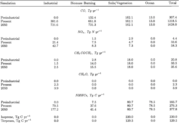
Table 1 gives the global surface emissions used in

MOZART for preindustrial, present-day, and future

(2050) conditions. Present-day emissions are similar to those used by Brasscur et al. [1998b]. The only update

to these emissions concerns the NO soil release based

Table 1. Preindustrial, Present-Day, and Future (2050) Global Emissions Used in MOZART a

Simulation Industrial Biomass Burning Soils/Vegetation Ocean Total

CO, Tg yr -• P reindust ri al 0.0 132.4 162.1 13.0 307.4 Present 381.6 661.8 162.1 13.0 1218.5 2050 721.6 731.3 162.1 13.0 1628.0 NO.• , Tg N yr -• Preindus t ri al 0.0 1.5 2.9 0.0 4.4 Present 21.4 7.5 4.7 0.0 33.6 2050 42.7 8.3 7.3 0.0 58.3 CH3 CO CH•, Tg yr- 1 Preindus t ri al 0.0 2.8 18.0 0.0 20.8 Present 1.5 14.0 18.0 0.0 33.5 2050 2.5 15.5 18.0 0.0 35.6 CH2 O, Tg yr- P reindust ri al 0.0 0.0 0.0 0.0 0.0 Present 2.3 0.0 0.0 0.0 2.3 2050 3.9 0.0 0.0 0.0 3.9 1 NMHCs, Tg C yr- Preindust ri al 0.0 7.5 80.7 78.5 166.7 Present 79.5 37.6 80.7 78.5 276.3 2050 177.2 41.4 80.7 78.5 377.8 Isoprene, Tg C yr -• 0.0 0.0 220.0 0.0 220.0 Terpenes, Tg C yr -• 0.0 0.0 129.5 0.0 129.5

aLightning NO., emissions are fixed to 7 Tg N in MOZART for both preindustrial, present-day, and future conditions.

32,340 HAUGLUSTAINE AND BRASSEUR: EVOLUTION OF TROPOSPHERIC OZONE

on Yienger

and Levy [1995]

which

totals 4.7 Tg N yr -•

instead of the 6.6 Tg N yr -• used in the earlier ver- sion of MOZART and based on MSller [1992]. For the

preindustrial simulation the industrial emissions are set

to zero. There is a high uncertainty on preindustrial biomass burning emissions. Owing to the lack of infor- mation, we make the simple assumption that the prein- dustrial emissions were only 20% of their present-day global value, with similar geographical and seasonal dis- tributions. Previous modeling studies have used similar assumptions, and reduced their global biomass burn- ing emissions to 10-25% of their present estimate [e.g.,

Wang and Jacob, 1998; Berntsen et al., 1997; Roelofs et

al., 1997]. These decreased emissions account for lower

population in the tropics at that period. It should be

noted, however, that changes in the emission patterns of emissions have also occured. Here again, little infor- mation is available even though it is believed that defor- estation has been more affected than savanna burning or boreal forest fires. These geographical differences are not considered in this study. An extreme case, with biomass burning emissions completely shut off, has also been considered to put some bounds to the problem, simulated and will be discussed below. Natural (i.e., vegetation, soils, and ocean) emissions are unchanged for all simulations. For NO soil emissions, as described by Yienger and Levy [1995], the emissions are modi- fied to account for fertilizer use in relation to changing

agricultural activities. The natural soil emissions cal-

culated with the model of Yienger and Levy [1995] to-

tal 2.9 Tg N yr -1, corresponding

to about 60% of the

present-day value of all soil emissions. Plate i shows

the annual NO soil emissions calculated by Yienger and Levy [1995] and used for the MOZART preindustrial and present-day simulations. The change in the geo- graphical distribution from the preindustrial to present occurs primarily through enhanced emissions in north- ern America, Europe, China, and India due to the appli- cation of fertilizer in these regions. As will be discussed later, this feature is particularly important when cal- culating preindustrial ozone, as soil emissions were the

major surface source of NOx around 1850.

Future emission estimates are based on the IPCC ref-

erence scenario IS92a [IPCC, 1992]. The assumptions, methodology, and results of the various 1992 IPCC

scenarios

(IS92a through

f) have been summarized

by

IPCC [1992] and are described in more detail by Pepper

et al. [1992].

New scenarios

(SRES) have

recently

been

proposed [IPCC, 2000] for the IPCC third assessment

report. A preliminary version of the SRES scenarios

has been used recently by Stevenson et al. [2000]. In this study, however, we use the 1992 scenarios since they have been used in several other modeling studies and can be regarded as a reference case for model in-

tercomparisons. IS92a is considered here as a business- as-usual scenario with moderated abatement measures

and is used for reference. New simulations using the

new SRES scenarios will be reported elsewhere. We consider in this study a time horizon of 50 years and

present the results for year 2050. Assumptions on pop- ulation and economic growth are key drivers of energy

use and overall industrial activity. These evolutions are

expected to vary significantly from one region to an- other in the future. Therefore not only the global emis- sions have been modified but also their geographical dis- tribution. This feature is of particular importance re- garding the photochemistry of ozone. The global emis-

sions, as adopted in the model, are modified accord-

ing to scaling factors provided for the different chemi- cal species and emission types according to IS92a. As reported by Pepper et al. [1992], these scaling factors are modified on the basis of four regions: OECD coun- tries, Russia/Eastern Europe, China/Centrally Planned

Asia, and other countries. Table i provides the result-

ing global emissions obtained for 2050, and Plate 2 il- lustrates the geographical distributions of total CO and NOx emissions for both present-day and 2050 condi- tions. This plate clearly shows the increase in surface emissions in Southeast Asia, India, and Central Amer- ica as a consequence of growing industrial activities. To a lesser extent, increased emissions are also predicted in Africa and South America, mainly as a consequence of enhanced biomass burning emissions. In the northern

hemisphere, emissions over the United States and Eu-

rope are slightly reduced due to the moderated abate-

ment measures assumed in the IS92a scenario.

In MOZART, as described by Brasseur et al. [1998b], the distribution of several long-lived species (03, NOz, HNO3, N205, CO, CH4, and N20) are prescribed above

60 mbar (or approximately

20 km altitude), according

to monthly and zonally averaged values provided by the middle atmosphere 3-D STARS model [Brasseur et al., 1997]. For all simulations the distributions of 03, NOz, HNO3, N205, and CO are unchanged above this alti- tude. However, in the lower stratosphere, the distribu- tion of these species can be affected by photochemistry

and transport. Note that version 1 of MOZART does

not account for chlorine and bromine chemistry in the stratosphere. Because of their long lifetime compared to the model integration time (i.e., 2 years), CH4 and N20 concentrations are scaled in the troposphere to their concentrations determined from ice core analyses for the preindustrial simulation and to their 2050 global concentrations as provided by IPCC [1992] for the fu-

ture simulation.

In order to investigate the contribution of the strato-

spheric influx to the calculated ozone levels in the tro-

posphere, a stratospheric ozone-like tracer is added in

MOZART. As described

by Hauglustaine

et al. [2001],

this tracer is imposed to be identical to the modeled real ozone above the model tropopause. Below the tropopause the photochemical production is set equal to zero, while a photochemical loss is attributed to ozone

HAUGLUSTAINE AND BRASSEUR: EVOLUTION OF TROPOSPHERIC OZONE 32,341

NOx Annual Soil Emission, Pre-lndustriol

": '• •• •i . ..:':.•.i:

...

• '

Min = 0.00e+00 Max = 3.26e+02

kg/km2/yr 4.0e+02 3.0e+02 2,0e+02 1,0e+02 7.0e+01 5.0e+01 3.0e+01 1.0e+01 5.0e+00 1.0e+00 5,0e-01 1.0e-01 5,0e-02 1.0e-02 1.0e-03 0.0e+00

NOx Annuol Soil Emission, Present Doy kg/km2/yr

i

:

:

!

i

!

i

i

•.o•+o•

: ... .•.r-...•

..,•..i,.•

. ..,.;

...

:

.

q

2.0e+02

'•; i

1.0e+02

•'•'•

i 3.Oe+01

:i

i

: 1.0e+01

I 1.0e-02

Min = 0.00e+00 Max = 4.35e+02

Plate 1. Annual NO soil emissions calculated with the model of Yienger and Levy [1995] for

preindustrial

and present-day

conditions

(kg N km -2 yr-1).

CO Emissions - Present

Min = 0.O0e+O0 Max = ½.Ole+O4

kg/km2/yr 3.5e+04 3.0e+04 2,5e+04 2.0e+04 1.5e+04 1.0e+04 7.5e+03 5.0e+03 2,5e+03 1.0e+03 0.Oe+00 CO Emissions - 2050 MOZART : :

Mln = O.00e+00 Max = 9.92e+O4

kg/km2/yr 3.5e+04 3.0e+04 2,5e+04 2.0e+04 1.5e+04 1.0e+04 7.5e+03 5.0e+03 2.5e+03 1.0e+03 0.Oe+00

NOx Emissions - Present

:'" i ."4• ;"'i t .

...

...

....

....

.,

...

• ...

: ...

:..;:

...

• ...

• ...

• ...

• ...

'MOZART

Min = 0.00e+00 Mox = 1.1..T•e+04

kgN/m2/yr 3.0e+03 2.8e+03 2.5e+03 2.2e+03 2.0e+03 1.8e+05 1.5e+03 1.2e+03 1.0e+03 7.5e+02 5.0e+02 2.5e+02 1.0e+02 O.0e+00

Plate 2. Present

and

future

(2050)

annual

surface

emissions

of CO (kg km

-2 yr -1) and NOx

32,342 HAUGLUSTAINE AND BRASSEUR: EVOLUTION OF TROPOSPHERIC: OZONE

Stratospheric 03 (%), Surface, July

Min = 3.3 Max = 91.6

MOZART

:' x .:

0. 10. 20. 30. 40. 50. 60. 70. 80. 90.

Stratosphedc 03 (%), 500 rob, July

M;n = 20.4 Max = 94.2 ., MOZART . o. lo. 20. 30. 40. 50. Stratospheric 03 (%), 300 mb, July Min = 20.9 Max = 100.0 60. 70. 80. 90. MOZART 0. 10. 20. 30. 40. 50. 60. 70. 80. 90.

Plate 3. Contribution of stratospheric ozone to the ozone distribution at the surface, 500 mbar, and 300 mbar calculated for July conditions (percent).

vapor, to reaction of ozone with OH and HO2, and to

reaction of ozone with NMHCs. Dry deposition at the surface is also considered for this so-called stratospheric ozone tracer. A similar definition for a stratospheric

ozone tracer has been used by Ro½lofs and Lelicv½ld [1997].

The contribution of the ozone influx from the strato-

sphere to the calculated tropospheric ozone levels is ca.1-

culated as the ratio between the stratospheric tracer

and the modeled real ozone. This ratio, expressed in percent, is illustrated for present-day conditions on Plate 3 for July conditions for three different altitude

levels. Over the continents in the northern hemisphere,

the stratospheric contribution is minimum in the bound-

ary layer (only a few percent) as, near the surface,

ozone is almost entirely photochemically produced from the release of its precursors by industrial and natural emissions. Similarly, minimum stratospheric contribu-

tions are calculated in the tropics (e.g., South America, Africa) where photochemical production from biomass burning and biogenic emissions of precursors prevails.

The photochemical influence is also clear in the midtro-

posphere (500 mbar) over most of the northern hemi-

sphere, where the stratospheric contribution represents

20-30% of the ozone level over polluted regions and 30- 50076 over oceanic regions. In the southern hemisphere

extratropics, however, the influence of stratospheric in-

put is dominant during this season and generally higher than 80% at all altitudes. Meridional transport of ozone originating from the stratosphere to the tropics, into

the South Pacific, South Atlantic, and Indian Oceans

is simulated with this model. At 300 mbar, high and

midlatitudes are located within the stratosphere. How-

ever, the contribution of photochemical production in the troposphere is still high in the tropics where strong

upward transport and convection prevail. The strato-

spheric tracer will be used in the following sections to provide a lower limit on preindustrial ozone background

levels.

3. Evolution of Tropospheric Ozone and

Its Precursors Since the Preindustrial

Era

3.1. Changes in Atmospheric Composition

For present-day conditions the calculated surface NO•

mixing ratio reaches more than 5 ppbv over Europe, eastern Asia, and North America. These high values are due primarily to fossil fuel emissions (Plate 4). In the biomass burning regions of Africa and South America the calculated mixing ratio is typically in the range 1-3

ppbv. As illustrated by Plate 4, preindustrial levels are

significantly lower over source regions. Over the conti- nents, biogenic soil emission is the main preindustrial surface source of NO•. The NO• patterns follow the dis- tribution of soil emissions with background values lower

than 40 pptv and maximum values of typically 300-500 pptv at northern midlatitudes where soil emissions are

high. The calculated preindustrial distribution of NO•

is less uniform in space than reported by Berntsen et

al. [1997]. These authors estimated mixing ratios gen- erally larger than 100 pptv in the boundary layer. In the

tropics the simulated preindustrial levels reach locally

500-1000 pptv due to maximum biogenic emissions in these regions (see Plate 2) and residual biomass burn- ing emissions. We find the preindustrial NO• distribu- tion in the boundary layer to be controlled primarily

by natural soil emissions at northern midlatitudes and

therefore very sensitive to assumptions made for these

emissions. It is therefore crucial to determine the nat-

HAUGLUSTAINE AND BRASSEUR: EVOLUTION OF TROPOSPHERIC OZONE 32,343

fertilizers [Yienger and Levy, 1995]. Uncertainties in estimating natural NOx from soils and from lightning will strongly affect the calculated preindustrial ozone

concentrations. A similar conclusion was reached by

Lelieveld and Dentenev [2000] for their 1860 simulation.

The calculated preindustrial and present-day CO dis- tributions at the surface are shown on Plate 4 for July conditions. Present-day values reach more than 200

ppbv in polluted regions in the northern hemisphere and in the tropics over biomass burning regions. An in- terhemispheric difference of more than 50 ppbv is calcu- lated with values of 100-150 ppbv north of about 50øN and background mixing ratios of 50-70 ppbv over the ocean in the southern hemisphere. Preindustrial mixing ratios are significantly lower with background levels in the range 20-40 ppbv in oceanic regions. Over the con- tinents, mixing ratios of 40-60 ppbv are predicted and mainly associated with CO biogenic emissions (soils) and production of CO through oxidation of biogenic hydrocarbons (i.e., isoprene and terpenes). In the trop- ics, due to important biogenic hydrocarbon emissions and residual biomass burning, maximum values of 60-

80 ppbv are calculated.

Preindustrial CO levels have been estimated from ice

cores in Antarctica (50-60 ppbv) and Greenland (90 ppbv) by Haan et al. [1996] and Haan and Raynaud [1998]. These studies suggest that carbon monoxide did not change significantly during the last 150 years in polar regions. Our calculated preindustrial CO levels sampled over a full annual cycle over Antarctica and Greenland are in the range 19-22 ppbv and 35-55 ppbv, respectively. These results are at odds with the ice core analyses. A similar disagreement has also been reached by other models [Wang and Jacob, 1998]. The Antarctic levels measured by Haan et al. [1996] are

also inconsistent with the lower preindustrial methane abundance. Possible contamination of the ice sample

during the experimental procedure is, however, not ex- cluded (J. Chappellaz, personal communication, 2000), and the polar ice core measurements are currently being

reexamined.

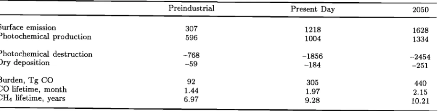
The CO global budget given in Table 2 indicates that the preindustrial CO burden, as calculated by MOZART, is 3 times lower than the current value, re- flecting lower direct surface emissions and a reduced photochemical production through CH4and NMHCs ox- idation. More abundant OH concentrations at prein-

dustrial times also contribute to lower CO densities.

A 16 day increase in the CO photochemical lifetime (from 1.4 to 2 months) is calculated from preindustrial to present. Similarly, the methane lifetime estimated by the model increases from 7 years at preindustrial times to 9.3 years for present-day cond;.tions. These changes in lifetime reflect the strong impact of human activi- ties on the oxidizing capacity of the atmosphere, with a global decrease of OH by 33% in the last 150 years.

The simulated preindustrial and present-day ozone surface mixing ratios are illustrated on Plate 5 for Jan-

uary and July conditions. The preindustrial levels over

the continents in the northern hemisphere range from a

minimum value of 5-15 ppbv in January, associated with chemical loss and dry deposition, to a summer value

reaching 10 ppbv in Europe and 20 ppbv in the cen-

tral United States where NO soil emissions and, conse-

quently, NOx preindustrial levels are at maximum (see Plate 4). In the southern hemisphere the preindustrial mixing ratios over the ocean ranges from only 4-8 ppbv in January due to chemical loss to values of 10-20 ppbv

in July associated with a seasonal maximum of influx

from the stratosphere (see Plate 3). The present-day distributions clearly emphasize a strong impact of an- thropogenic activities on ozone levels at a global scale. Maximum Oa mixing ratios reaching 50-60 ppbv are calculated over polluted regions (i.e., northern Amer- ica, Europe, and Southeast Asia) during summer in the northern hemisphere. Export of ozone rich air from the United States and from Europe to the northern At- lantic is visible in July, with ozone mixing ratios reach-

ing 25-30 ppbv in the export plumes over the ocean.

The background ozone levels calculated over the ocean in the southern hemisphere have increased by 5-10 ppbv

in comparison [o preindustriai values.

Table 2. Annual

Budget

of Carbon

Monoxide

in the Troposphere

(Below

250

mbar)

Calculated

by MOZART

for Preindustrial,

Present-Day,

and

Future

(2050)

Conditions,

and

Atmospheric

Lifetime

of CO and

CH4

a

Preindustrial Present Day 2050

Surface emission 307 1218 1628 Photochemical production 596 1004 1334 Photochemical destruction -768 -1856 -2454 Dry deposition -59 -184 -251 Burden, Tg CO 92 305 440 CO lifetime, month 1.44 1.97 2.15 CHq lifetime, years 6.97 9.28 10.21 a Units are in Tg CO yr -1

32,344 HAUGLUSTAINE AND BRASSEUR: EVOLUTION OF TROPOSPHERIC OZONE

Montsouris (5ON, 2E), 1876-188,5

• 301

... I • 3o

n-

15

! n-

15

• 301

...

• 15

•e

1

Mont Ventoux (44N, 4E), 1891 - 1905

• 25

o

n- 15

J F M A M J J A S 0 N D

Pic du Midi (43N, OE), 1881-1909

•> 30 ...

•25 • •] B•

_{* * * * *}

-

.,>

30

...

iI

Hong Kong (22N, 114E), 1872-1874

... I I i i i i i i i i i J F M A M J J A S 0 N O > 30 ,', 25 ._6 20 n- 15 .-• 10 x • 5 o 0 Oaxaca (17N, 96W), 1892-1899 ... i I i i i i i i i i i J F M A M J J A S 0 N O

Figure 1. Seasonal cycle of surface ozone for the preindustrial period (ppbv). Dots, measure- ments (see text for details); box-wisker plot, model monthly mean and standard deviation; scars, stratospheric ozone contribution; open diamon•ts, calculated ozone neglecting biomass burning

emissions.

Surface ozone levels recorded during the nineteenth from various sources. In particular, relative humid- century have been re-evaluated in the literature and re- ky, temperature, and also wind speed can affect the

ported

at various

sites [see,

e.g., Mavenco

et al., 1994]. ozone

reading.

Other pollutants

can also

increase

(e.g.,

These

historical

measurements

in ambient

air were

made H202, HO2, NO2, PAN), or decrease

(SO2, NH3) the

using the Sch6nbein paper method. This technique is ozone reading. For these reasons, the possibility of de- not strictly quantitative and suffers from interference riving reliable information on past ozone levels from the

HAUGLUSTAINE AND BRASSEUR: EVOLUTION OF TROPOSPHERIC OZONE 32,345 > 30 o. 25 ß -• 20 n. 15 .c_ 10 .x_ m 5 o 0 Manila (14N, 120E), 1878-1882 ... > 30 o. 25

It

.:_-

E•

B B

0 0 0 0 00.

>

30[

...

3 301

...

.=-

-

Figure 1. (continued)

Schanbein technique is controversial. However, several Hobart (Tasmania) are taken from Payella et al. [1999]. authors have used proper correction techniques and cali- The preindustrial ozone mixing ratios calculated with bration procedures to reassess these historical levels and MOZART at the historical sites are compared to the derive useful information. Bearing these limitations in measurements on Figure 1. As noted by Payella et mind, in this study we compare the measurements to al. [1999], the error bar on the observed value is large the model results to provide some constraint on our (4-5 ppbv or larger). The strataspheric ozone tracer calculations. The nineteenth century ozone levels con- (see section 2) at the location is also shown for cam- sidered here are taken from Volz and t(ley [1988] for parison. We find a fairly good agreement between Montsouris (France), Artrossi et al. [1991] for Man- model and measurements at several extratropical and calieri (Italy), Sandtoni et al. [1992] for Montevideo midlatitude stations previously used for model evalu-

(Uruguay),

and Cordoba

(Argentina),

and Marerico

et ation. This is particularly

the case

for the European

al. [1994]

for the Pic du Midi (southwestern

France). stations

of Montsouris,

Moncalieri,

and in the south-

Historical data at Manila (Philippines), Rio de Janeiro ern hemisphere at Montevideo and Adelaide. At these

(Brazil), and Oaxaca

de Juarez

(Mexico)

are taken

from stations,

fairly constant

mixing ratios of 5-10 ppbv are

Sandtoni

and Artrossi

[1994]. Measurements

reported obtained

throughout

the year. This is clearly in con-

at Vienna (Austria), Mont Ventoux

(France),

Nemuro trast with typical seasonal

cycles

simulated

for present,-

and Tokyo (Japan), Coimbra (Portugal), Hang Kong, day conditions

exhibiting maximum mixing ratios as-

32,346 HAUGLUSTAINE AND BRASSEUR: EVOLUTION OF TROPOSPHERIC OZONE

met [Hau#lustaine

et al., 1998a]. During winter and

that ozone

is mainly

from stratospheric

origin. During

summer an ozone enhancement of about 5 ppbv is cal-

culated

and associated

with biogenic

emissions

of pre-

cursors. At the two southern hemisphere stations of

Cordoba

and, to a lesser

extent, Hobart, a fairly good

agreement is reached except during the summer period. A fairly good agreernent is also obtained at the altitude

site of Mont Ventoux

(1910 m). However,

during

win-

ter and spring, an overestimate of 5-10 ppbv points to-

ward an excess

contribution

from stratospheric

input in

the model. At this site the stratospheric

tracer

clearly

shows

a large contribution

of the stratospheric

influx

from November to May. A different picture is obtained

at the second

altitude

site of Pic du Midi (2860

m),

where a ozone

is systematically

overestimated

by 10-

15 ppbv. A similar disagreement has been obtained at

this site by Wang and Jacob

[1998].

During

winter and

spring the contribution of stratospheric ozone at this

altitude is even larger than the measurements

by 5-8

ppbv. This feature would point toward an overestimate

of stratospheric

influx in MOZART. During summer

a

tropospheric

ozone

excess

is simulated.

Absence

of dry

deposition

in the model

at this altitude

(associated

with

for the disagreement.

However,

according

to Marenco

et al. [1994],

the Pic du Midi data are representative

of free tropospheric

air. A systematic

disagreement

is

obtained in the tropics at continental stations. At Oax- aca, Manila, Luanda, and Rio the measurements seem to provide mixing ratios close to 5 ppbv and even less,

while the modeled

values

are in the range 10-15 ppbv

or even as high as 20 ppbv. In order to investigate the

potential role played by the residual

biomass

burning

emissions

(20% of present-day

value), a preindustrial

case, in which biomass burning emissions are omitted, has been performed. As shown by Figure 1, even in this extreme case, the calculated mixing ratios still overes-

timate the measurements

by 10-15 ppbv in the tropics.

For the station of Luanda the comparison has, however, improved during August-November. For the stations of

Vienna,

Nemuro,

and Tokyo,

measured

values

are larger

than model results regardless of the season. The rea- sons for this disagreement are not clear. A relatively good agreement is reached with this model at midlati- tude locations. This contrasts with the systematic over-

estimate

reported

by previous

studies

[Berntsen

et al.,

1997; Wang

and Jacob,

1998;

Mickley

et al., 2001]. The

calculated preindustrial ozone levels at these altitudes are found to be particularly sensitive to the NO soil

emissions used in the model. Natural soil emissions appear crucial for the simulation of surface ozone for

pristine conditions. In the tropics a systematic overes-

timate is reached

with this model. We note, however,

that the observed

levels

of only 5 ppbv are surprisingly

low and possibly reflect problems with the ozone read-

ing from the Sch6nbein paper. Again, we would like to stress the large error bar associated with the historical data. Disagreement (or agreement) noted in Figure 1 may well be insignificant.

The modeled relative ozone change since preindus- trial times (present to preindustrial ozone ratio) indi- cates a general increase of surface levels by more than a factor of 2 during July in the northern hemisphere when photochemical production is a maximum (Plate 6). The ozone concentration increase reaches more than a factor of 5 over polluted regions. Export of ozone (in- crease by a factor of 3-4) to the northern Atlantic and to northern polar latitudes is also visible. In January, ozone increases roughly by 50-80% over the ocean in the northern hemisphere and by a factor of 2- 3 over the continents. Over the ocean in the southern hemisphere the Oa concentration increases by only 10-20% in July

(when transport

from the stratosphere

dominates)

and

by 30-50% in January. The ozone increase associated with biomass burning is also visible in the tropics with local increases reaching a factor of 2-3. The ozone in- crease is also visible in the midtroposphere (500 mbar) in the northern hemisphere. In July, export of ozone from polluted regions is responsible for a general in- crease reaching a factor of 2-3. A similar relative ozone

increase

has also been reported

by Levy et al. [1997].

In the tropics and subtropics, due to vigorous upward transport, the ozone density increases by 70-100% up to 200 mbar where the impact on climate is the largest

[Lacis

et al., 1990;

Hauglustaine

and Granier,

1995].

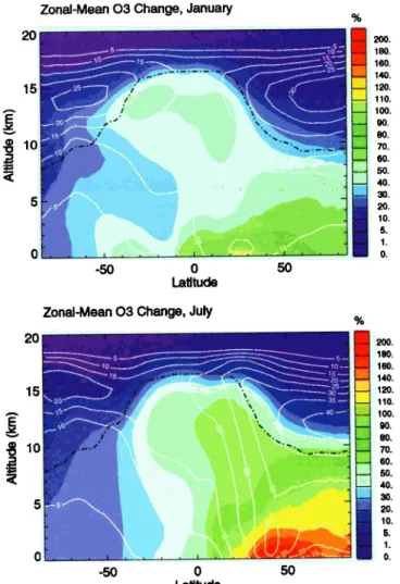
Plate 7 provides a different perspective on the ozone change as a function of altitude, and shows the increase in the zonal mean distribution of ozone for January and July conditions. As shown earlier, the maximum ozone

increase is found at midlatitudes in the northern hemi-

sphere during July and reaches a factor of 3 at the sur- face. Transport from the polluted boundary layer to the mid and upper troposphere is visible. In partic- ular, in both seasons a secondary maximum reaching more than 50% is calculated in the tropical upper tro- posphere. The ozone change is in line with the results presented by Berntsen et al. [1997] and Stevenson et al. [1998] with calculated ozone increases in the upper tro- posphere reaching 15 ppbv and 30 ppbv, respectively, in the northern hemisphere during January and July, and 15-20 ppbv in the tropics. At the surface, ozone increases by 25-30 ppbv at northern midlatitudes and by less than 10 ppbv in the southern hemisphere.

In most of these previous studies the ozone influx

from the stratosphere remained unchanged between pre- industrial and present-day conditions [Wang and Jacob, 1998; Stevenson et al., 1998; Mickley et al., 1999]. In other cases the ozone mixing ratios in the stratosphere were held constant [Brasseur et ai., 1998a; Berntsen et al., 1997; Roelofs et al., 1997]. In MOZART the in- crease in tropospheric ozone concentration and subse- quent transport through the tropopause is responsible for an increase in the lower stratosphere in all seasons.

HAUGLUSTAINE AND BRASSEUR: EVOLUTION OF TROPOSPHERIC OZONE 32,347

Pre-lndustdai NOx mixing ratio, pptv, Surface, July

Mm = 2 74e-01 Max = 9 97e+02

MOZAR'[

. •

0. 20. 40. 60. 80. 100. 300. 500. 1000. 2000. 3000. 5000.

Present-Day NOx mixing ratio, pptv, Surface, July

Min = 9.81e-01 Max = 1.68e+O4

MOiART

Pre-lndustrial CO mixing ratio, ppbv, Sudace, July

•l•n = 1.94e+01 Max = 8.20e•1

MOZART

.

Present-Day CO mixing ratio, ppbv, Surface, July

Min = 5.62e+01 Max = 2.85e+02

0. 20. 40. 60. 80. 100. 300. 500. 1000. 2000. 30(10. SO00. o. 20. 40. 60. 80. lOO. 150. 200. 250. 300.

Plate 4. (left) Surface

distribution

of NOx calculated

in July for preindustrial

and present-day

conditions

(pptv). (right) Surface

distribution

of (•0 calculated

in July for preindustrial

and

present-day conditions (ppbv).

Pre-lndustriai 03 mixing ratio, ppbv, Surface, January

Min - 3.87e+00 Max = 2.599,O1

I I ]

o. 2. 4 6. s. t0. 15. 20. 25. 30. 40. 50. 60.

Pre-lndustrial 03 mixing ratio, ppbv, Surface, July

Mtn = 2.03e+00 Max = 2.63e,01

ß . ß • ... 4 ... • ... -' ... .. i ... • ... i ... • ... • ... •.. ... :MOZART : . : :. • : : : O. 2. 4. 6. 8. 10. 15. 20. 25. 30. 40. 50. 60.

Present-Day 03 mixing ratio, ppbv, Surface, January

Min • 6.619+00 Max .. 4.17e+01

... -. ... : ... : ... i ... ! ... • • : : ' • -i ... ; ... : i i ' ... i ... i ... o ... i ... o ... ... i ... i ... : i : i ! i ]_ 1__ ..! __!__! _1 I I _ I ! ! ! I 0. 2. 4 6. 8, 10. IS. 20. 25. 30, 40. 50. 60.

Present-Day 03 mixing ratio, ppbv, Sudace, July

Mm = 4.58e+00 Max = 7.80e+01

I

O. 2. 4. 6. 8. 10. 15. 20. 25. 30. 40. 50. 60.

Plate 5. Surface distribution of 03 calculated in January and July for preindustrial and present- day conditions (ppbv).

32,348 HAUGLUSTAINE AND BRASSEUR: EVOLUTION OF TROPOSPHERIC OZONE

Present-Day to Pre-lndustria103 ratio, Sudace, January

Mm = 1.23e+00 Max = 4.70e+00

MO;•ART

Present-Day to Pre-lndustria103 ratio, Surface, July

Min = 1.24e+00 Max = 9.19e-K)0

MOZART

ll ll

1.0 1.1 1.2 1.3 1.4 1.5 1.6 1.7 1.8 1.9 2.0 3.0 4.0 5.0 1.0 1.1 1.2 1.3 1.4 1.5 1.6 1.7 1.8 1.9 2.0 3.0 4.0 5.0

Present-Day to Pre-lndustrial 03 ratio, 500 mb, January

Min = 1.12e+00 Max = 1.67e+00

MOZART

ß

Present-Day to Pre-lndustrial 03 ratio, 500 mb, July

Min = 1.15e+00 Max = 2.51e+00

MOZART ß 1 1.0 1.1 1.2 1.3 1.4 1.5 1.6 1.7 1.8 1.9 2.0 3.0 4.0 5.0 1 1.0 1.1 1.2 1.3 1.4 1.5 1.6 1.7 1.8 1.9 2.0 3.0 4.0 5.0

Present-Day to Pre-lndustrial 03 ratio, 200 mb, January

Min = 1.03e+00 Max = 1.67e+00

MOZART

Present-Day to Pre-lndustria103 ratio, 200 mb, July

Min = 1.02e-K)0 Max = 1.88e+00

MOZART

1.0 1.1 1.2 1.3 1.4 1.5 1.6 1.7 1.8 1.9 2.0 3.0 4.0 5.0

I ll

1.0 1.1 1.2 1.3 1.4 1.5 1.6 1.7 1.8 1.9 2.0 3.0 4.0 5.0

Plate 6. P•elative ozone increase from pre-indutrial to present calculated at the surface, 500 mbar, and 200 mbar for January and July conditions.

HAUGLUSTAINE AND BRASSEUR: EVOLUTION OF TROPOSPHERIC OZONE 32,349

20

15

Zonal-Mean 03 Change, January

0

I _ 2 ....

t

I i , , ,, I

Zonal-Mean 03 Change, July

200. 180. 160. 140. 120. 110. 100. 90. 80. 70. 60. 50. 40. 30. 20. 10. 5. 1. O. • , o-...•.. ,. ,-- - -% 20--- 140. '• •' •, 25-- \ 3o --• 120.

x-.2o

•-'•--'ff /'

•

35•

110.

•

10.

ics, in agreement with more sophisticated definitions

[see, e.g., Hoi•lca, 1998]. The resulting change in the

tropospheric column reaches maximum values of 30-40

Dobson units (DV) (20 DV in zonal mean) over the pol- luted regions (40ø-50øN) of the northern hemisphere in

July. A strong export of ozone to polar regions is sim- ulated by the model and results in an ozone increase

reaching 16-18 DU in zonal mean at northern polar lat- itudes during summer. In January a more uniform in-

crease of 10 DU or less is calculated in the southern

hemisphere, and a column increase of 8-12 DU is cal- culated in the northern hemisphere. In the tropics an ozone increase associated with a peak in biomass burn-

ing activity reaching 8-10 DU in zonal mean is predicted in October (10ø-20øS). The seasonal and geographical

distributions of the tropospheric ozone column increase

are in good agreement with the previous estimate by Kichl ½t al. [1999]. In particular, a similar maximum is predicted at mid and high latitudes during summer in the northern hemisphere and in the tropics during the peak in biomass burning activity (i.e., September- October). We note, however, that the amplitude of the maximum is larger in the previous study by about 2-8

DU in comparison to our estimate. Different preindus- trial levels are a possible source of discrepancy with this previous work.

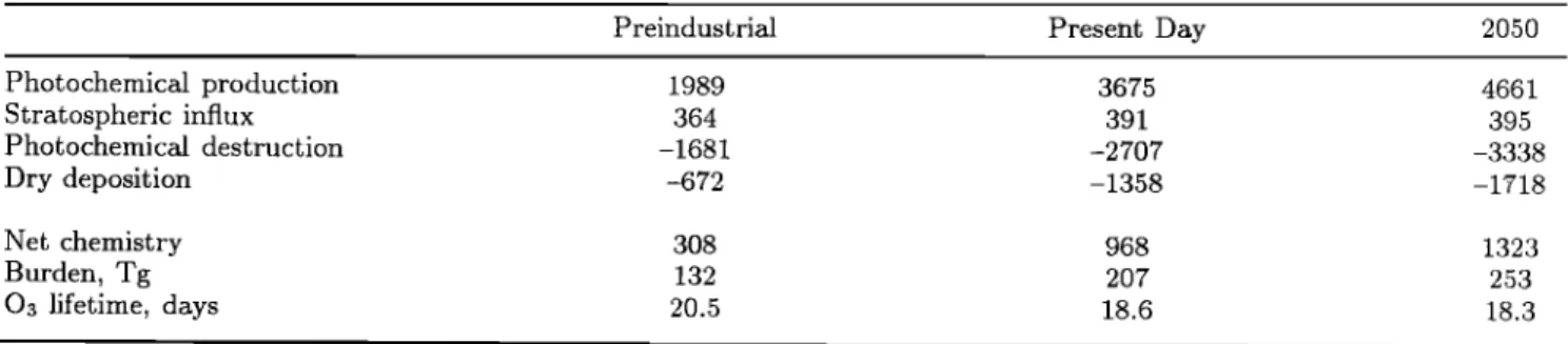
Table 3 provides the calculated tropospheric ozone

budgets (up to 250 mbar) for preindustrial and present- day conditions. The impact of anthropogenic activities on ozone photochemical production induces an 85% in- Plate 7. Zonal mean change in ozone from pre-

indutrial to present for January and July conditions. Shaded contours give the change in percent, and solid contours give the increase in ppbv.

These maxima reach 20-40 ppbv in absolute values (less than 10-20%). A similar conclusion has been reached by L½licv½ld and Dentenet [2000]. It should be noted

that the actual version of the MOZART model does not

include chlorine and bromine chemistry in the strato-

sphere. Therefore, in the present study, we focus on tropospheric ozone changes only and do not consider the impact of stratospheric ozone changes on the chem- istry of the troposphere. As illustrated by Kiehl et al. [1999], the zonal and annual mean ozone concentration in the lower stratosphere at high latitudes has decreased by typically 10-20% due to stratospheric ozone catalyt-

ical destruction.

Plate 8 shows the change in the tropospheric ozone column for January and July, and Figure 2 shows the corresponding seasonal evolution as a function of lati- tude. We adopt here a thermal definition of the tro- popause as the lowest model level at which the tem-

perature

vertical gradient

decreases

below 2 K km -1

The resulting tropopause height, illustrated on Plate 7, ranges from 8 km in polar regions to 16 km in the trop-

Tropospheric O• Column Change since Pre-lndustrial, January DU

MOZART

'Min'•'i•De+oo ' Max = 1.29e+•11

30. 28. 26. 24. 22. 20. 16. 14. 12. 10. 8. 6. 4, 2, 0.

Tropospheric O• Column Change since Pre-lndustrial, July DU

IMOZART Min = 1.93e+O0 30. 28, 26. 24. 22. 20. 18, 16. 14. 12. 10. 8. 6. 4. 2, 0.

Plate 8. Tropospheric ozone column increase from pre- indutrial to present calculated for January and July conditions (DU).

32,350 HAUGLUSTAINE AND BRASSEUR: EVOLUTION OF TROPOSPHERIC OZONE

Ozone SW Radiatwe Forcing Since Pre-industrial - Annual W/m2

0.26 0.24 0.22 0.20 0.18 0.16 0.14 0.12 0.10 0.08 0.06 0.04 0.02 0.00

Ozone LW Radiative Forcing Since Pre-industrial - Annual

I•lin = 5.94•3 M•: 8.12e•)1 W/m2 0.90 0.85 0.80 0.75 0.70 0.65 0.60 0.55 0.50 0.45 0.40 0.35 0.30 0.25 0.20 0.15 0.10 0.05 0.00

Ozone Net Radiative Forcing Since Pre-industrial - Annual W/m2

0.90 0.85 0.80 0.75 0.70 0.65 0.60 0.55 0.50 0.45 0.40 0.35 0.30 0.25 0.20 0.15 0.10 0.05 0.00

Plate 9. Annual mean tropospheric

ozone

radiative

forcing

at the tropopause

calculated

from

pre-indutrial

to present

(W m-2). (top) Shortwave

forcing,

(middle)

longwave

forcing,

and

(bottom)

total forcing

(shortwave

plus

longwave).

Note the different

color

scale

of the SW