A non-intrusive reduced basis approach for parametrized heat transfer problems

(1)

HAL Id: hal-01897395

https://hal.archives-ouvertes.fr/hal-01897395

Submitted on 9 Jun 2021

HAL is a multi-disciplinary open access archive for the deposit and dissemination of sci-entific research documents, whether they are pub-lished or not. The documents may come from teaching and research institutions in France or

L’archive ouverte pluridisciplinaire HAL, est destinée au dépôt et à la diffusion de documents scientifiques de niveau recherche, publiés ou non, émanant des établissements d’enseignement et de recherche français ou étrangers, des laboratoires

A non-intrusive reduced basis approach for parametrized

heat transfer problems

Rachida Chakir, Yvon Maday, Philippe Parnaudeau

To cite this version:

Rachida Chakir, Yvon Maday, Philippe Parnaudeau. A non-intrusive reduced basis approach for parametrized heat transfer problems. Journal of Computational Physics, 2019, 376, pp.617-633. �10.1016/j.jcp.2018.10.001�. �hal-01897395�

(2)

A non-intrusive reduced basis approach for parametrized heat transfer problems

R. Chakir1 _{, Y. Maday} 2,3,4 _{and P. Parnaudeau}2,3

mail : rachida.chakir@ifsttar.fr; maday@ljll.math.upmc.fr; philippe.parnaudeau@univ-poitiers.fr

Abstract

Computation Fluid Dynamics (CFD) simulation has become a routine design tool for i) predicting accurately the thermal performances of electronics set ups and devices such as cooling system and ii) optimizing configurations. Although CFD simulations using discretization methods such as finite volume or finite element can be performed at different scales, from component/board levels to larger system, these classical discretization techniques can prove to be too costly and time consuming, especially in the case of optimization purposes where similar systems, with different design parameters have to be solved sequentially. The design parameters can be of geometric nature or related to the boundary conditions. This motivates our interest on model reduction and particularly on reduced basis methods. As is well documented in the literature, the offline/online implementation of the standard RB method (a Galerkin approach within the reduced basis space) requires to modify the original CFD calculation code, which for a commercial one may be problematic even impossible. For this reason, we have proposed in a previous paper, with an application to a simple scalar convection diffusion problem, an alternative non-intrusive reduced basis approach (NIRB) based on a two-grid finite element discretization. Here also the process is two stages: offline, the construction of the reduced basis is performed on a fine mesh; online a new configuration is simulated using a coarse mesh. While such a coarse solution, can be computed quickly enough to be used in a rapid decision process, it is generally not accurate enough for practical use. In order to retrieve accuracy, we first project every such coarse solution into the reduced space, and then further improve them via a rectification technique. The purpose of this paper is to generalize the approach to a CFD configuration.

Keywords : Non-intrusive method; Reduced basis method; Parametric studies; Heat transfer; CFD.

1. Introduction

During the past fifty years electronic devices and systems kept becoming smaller and smaller, this growing need for miniaturization led to an increasing high heat production. To avoid any possible failure or malfunction of electronics devices and ensure their reliability, it is essential to maintain the temper-ature of the electronic components below an acceptable upper limit. Cooling of electronic systems is consequently essential in controlling the component temperature and avoiding any hot spot. Designing cooling systems for miniaturized electronics devices presents difficult challenges to mechanical engineers and analysts. Average while, computational modeling is gaining popularity, particularly Computation

1

Université Paris Est, IFSTTAR, 10-14 Bd Newton, Cité Descartes, 77447 Marne La Vallée Cedex, France

2

CNRS, UMR 7598, Laboratoire Jacques-Louis Lions, F-75005, Paris, France

3_{UPMC Univ Paris 06, UMR 7598, Laboratoire Jacques-Louis Lions, F-75005, Paris, France} 4

Institut Universitaire de France and Division of Applied Mathematics, Brown University, Providence, RI, USA

*Manuscript

(3)

Fluid Dynamics (CFD) modeling which has become a routine design tool for predicting accurately ther-mal performance of electronics cooling system. Although CFD modeling can be used at different scales, from component/board levels to larger system, classical discretization techniques such as finite volume or finite element methods can prove to be limited by memory space and long calculation times, which can be problematic. Inexpensive and accurate computational tools to predict the fluid flow and heat transfer can be very useful, specially when thermal analysis is done at the end of the design process where time constraints are greatest, hence our focus on model reduction and particularly to reduced basis methods (see [9, 14, 17, 19]).

Reduced basis method exploits the parametric structure of the governing PDEs to construct rapidly, convergent and computationally efficient approximations. Previous work on the reduced basis method in numerical fluid dynamics has been carried out by [12, 16, 20] and more particularly for the Navier-Stokes equations [7, 18, 23, 27, 28] which requires treatment of non-linearity and non-affine parametric dependence. More recent works with turbulent flows can be found in [2, 26]. Let σ be a set of parameters associated to our physical system, these methods rely on the fact that when the parameters vary, the manifold of solutions is often of small (Kolmogorov) dimension. In this instance, there exists a set of N particular values of σ taken in D (the parameter space) from which one can build a basis. This basis,

called reduced basis, is made of the solutions u(σ1), · · · , u(σ_N) and can approach any solution u(σ),

σ _{∈ D. Thus, when the σ}i are well chosen5, the size of the reduced basis is much smaller compared to

the number of degrees of freedom of the problem discretized by a classical method (finite element, finite volume, or other). The standard reduced basis method is a Galerkin approach within the reduced basis approximation space, thus the reduced basis approximation of the “truth” solution is obtained by the resolution of a small dimensional linear system. One of the keys of this technique is the decomposition of the computational work into offline/online stages. However, the decomposition of the matrices into of-fline/online pieces requires modifying the calculation code, leading to an intrusive procedure. Examples of the standard reduced basis method applied to heat transfer problems can be found in [8, 21, 24, 25]. In some situation — with a commercial CFD code for example – it is not possible to perform all the offline computations required to have a inexpensive and fast online stage. For this reason, we proposed to use an less intrusive reduced basis method, introduced in [3, 4], where coarse triangulations are used to compute coarse approximation during the online stage. Recently, other non-intrusive Reduced Order Methods (ROM) for fluid dynamics have been proposed [5, 29], those ROM are based on proper orthog-onal decomposition and Radial Basis function (RBF) to compute the coefficients of the reduced model. During the online computation, for any given (untrained) parameter an interpolation approach using RBF as interpolation functions is used to estimate the coefficients of the POD decomposition. As in our method we use coarse triangulations to compute coefficients of the RB decomposition and then further improve them via a rectification technique, keeping a physical meaning to the approach. The aim of this paper is to provide tests to validate and generalize our method for heat transfer problems. In Section 2, we provide a brief introduction to reduced basis methods and the methodology of the non-intrusive reduced basis method. In Section 3, we give a brief description of simple models of cooling devices; we formulate the physical system, the governing equations and boundary conditions. In Section 4, we discuss our numerical experimentations and present the results and conclusions.

5

(4)

2. Methodology

Let us consider the nonlinear parametrized PDEs describing our physical system, over a bounded

domain Ω ⊂ Rd_{, d = 2 or 3. In these governing equations, θ represent the temperature, u}

i the

components of the velocity vector field u in the xi-directions , p the pressure and σ is a set of np

parameters related to physical properties or boundary conditions. We denote by D ⊂ Rnp _{the set of}

parameters.

We now introduce the variational formulation of our parametrized PDEs : I

for a given σ ∈ D, find (θ, u, p) ≡ (θ(σ), u(σ), p(σ)) ∈ X × Y × Q such that

F(θ, u, p ; T, v, q; σ) = (0, 0, 0)t_, _{∀ (T, v, q) ∈ X × Y × Q,} (1)

where F is a functional with the appropriate properties, X, Y and Q are appropriate functional spaces.

Let {Th}h be a family of regular triangulation of Ω, we denote by Xh, Yh and Qh finite element

approx-imation subspaces of respectively X, Y and Q over Th. The discrete velocity space Yh and the discrete

pressure space Qh are chosen in order to satisfy the inf-sup condition [6, 13, 22].

The finite element discretization of (1) is as follows : I

for a given σ ∈ D, find (θh, uh, ph) ≡ (θh(σ), uh(σ), ph(σ)) ∈ Xh× Yh× Qh such that

F(θh, uh, ph; T, v, q; σ) = (0, 0, 0)t, ∀ (T, v, q) ∈ Xh× Yh× Qh, (2)

For significantly fine meshes Th and adequately chosen discretization spaces Xh, Yh and Qh, the

con-forming finite element solution (θh, uh, ph), solution to (2), is accurate enough to be considered as a good

approximation of the exact solution, named “truth solutions”. However, because of the high dimension of the associated discretization spaces, solving the finite element problem (2) with different values of σ can prove to be too costly and time consuming.

The idea of reduced basis methods is to provide an economical and accurate approximation to the “truth”

approximation (θh, uh, ph) by using approximation spaces made up of few suitable samples of solutions

to the parametrized PDEs. This relies on the fact that when the parameters vary, the set of solutions is often of small Kolmogorov width, thus implying that the manifold of all solutions can be approximated within a (small) finite space of well-chosen solutions to the parametrized problem (2). In that case,

there exists a set of parameters SN = (σ1, σ2,· · · , σ_N) ∈ DN such that for any σ ∈ D, the truth

solution can be approximated by a linear combination of the particular solutions associated to σi ∈ SN.

To distinguish each physical component (temperature, velocity and pressure), we add superscripts θ, u

or p in our notation, for example we denote by (σθ

1, σ2θ, ,· · · , σθ_Nθ) the set of parameters — with size Nθ

— used to generate the reduced basis approximation space associated to the temperature component of the solution. For each physical component, we introduce the associated reduced basis approximation spaces as X_hN _{= span{θ}h(σiθ), 1 ≤ i ≤ Nθ} = span{φθi,1 ≤ i ≤ Nθ}, Y_hN _{= span{u}h(σ u i), 1 ≤ i ≤ N u } = span{φu i,1 ≤ i ≤ N u }, QN_h _{= span{p}h(σpi), 1 ≤ i ≤ Np} = span{φ p i,1 ≤ i ≤ Np}, where the 1φθ_i2 i ∈ Xh, (φ u i)i ∈ Yh, (φ p i)i ∈ Qh are H 1

-orthonormal basis sets (obtained respectively

from1θh(σiθ)

2

i, (uh(σ

u

i ))i and (ph(σpi))i by a orthogonalization process), called reduced basis functions.

The standard reduced basis method consists in a Galerkin approach within the low dimensional spaces X_hN, YN

(5)

I

for a given σ ∈ D, find (θN

h, uNh, pNh) ∈ XhN × YhN × QNh such that

F(θN

h , uNh , pNh ; T, v, q; σ) = (0, 0, 0)t, ∀ (T, v, q) ∈ XhN× YhN × QNh.

(3) Note that, in order to ensure stable, good approximation of the pressure, supremizer-enrichment of the

velocity reduced basis space may be performed, see for example [6, 13, 22]6_.

One of the key ingredients of the method is the decomposition of the computational work into offline and online stages. During the offline stage the reduced basis functions are computed — providing the above

defined spaces XN

h , YhN, QNh — as well as all parameter-independent quantities. This is an expensive

stage that is done only once, whereas parameter-dependent quantities are computed during the online stage together with the resolution to (3). Considering that the dimension of the reduced basis space is quite smaller compared to the finite element one, solving the reduced problem (3) is much less expensive than the “truth” finite element problem (2).

The construction of the associated discrete system to be solved is thus classically the corner stone of the global process. Indeed, since the construction of the reduced discrete system associated to the

variational form F(θN

h, uNh, pNh ; T, v, q; σ) has to be done for each new value of σ, to perform efficiently

the online stage, one has to be able to isolate the parametric contributions. Thus, all σ-independent quantities, high dimensional matrices and vectors used in the construction of the reduced discrete system are computed only once and saved during the offline stage. This part of the offline stage requires entering and modifying the simulation code used to compute the truth finite element approximations, leading to an intrusive method, which can be problematic. When the simulation code is locked and used as a black box — which is often the case in the industrial framework — the parametric decomposition is not possible, which prevent us from building each new reduced discrete system quickly for a new value of σ. This take away the benefit of the reduced basis method, thus to overcome it, we propose to use an alternative method, less intrusive, where coarse triangulations are used to compute finite element solutions during the online stage. These “coarse” approximations are projected into the reduced basis

approximation spaces XN

h , YhN, QNh, and then improve via a rectification technique introduced in [3, 4].

All these improvements after the coarse approximation is computed can be done in a different, more versatile code than the one used to do the simulation.

Let {TH}H be a family of “coarse” regular triangulation of Ω, such that H >> h, we denote by XH, YH

and QH the coarse finite element spaces associated to this mesh, and (θH, uH, pH) the “coarse” finite

el-ement approximation. Since the computation of the “coarse” finite elel-ement approximation, for H >> h is less expensive than the “truth” approximation, using the simulation code — during the online stage — with the mesh size H (chosen adequately) to construct a reduced solution is still cheap enough. In order to understand our non-intrusive reduced basis method, let us indicate that the idea of standard reduced basis methods (3) is to compute an inexpensive and accurate approximation of the projection

of the solution (θh(σ), uh(σ), ph(σ)) on XhN× YhN× QNh, by evaluating the coefficients appearing in the

decomposition of θN_h(σ), uN_h (σ) and pN_h(σ) in the basis1φθ_i2

i, (φ

u

i)i and (φ

p

i)i.

The best linear combination – measured in H1

-norm – of the reduced basis functions is provided by

the H1

-orthogonal projection

In our method, an alternative linear combination of the reduced basis functions has been chosen, using

6

However, in our context, we are not much interested here in the precise value of the pressure that is (only) a Lagrange multiplier to the divergence free condition), thus using the fact that the reduced velocity space is composed of divergence free functions the pressure does not even appear in the reduced set of equations (3), if no supremizer for the pressure space is added to XN

(6)

the optimal coefficients {βjθ,h(σ)}1≤j≤Nθ and {β

u,h

j (σ)}1≤j≤Nu involved in the L

2

-orthogonal projection

of θh(σ) on XhN and uh(σ) on YhN. As shown in [3, 4], these coefficients, defined as follows

βθ,h_i (σ) = 1θh(σ), φθi 2 L2, and β u,h j (σ) = 1 uh(σ), φ u j 2 L2 with 1 ≤ i ≤ N θ and 1 ≤ j ≤ Nu , (4) are still good enough but require the knowledge of the fine solution intervening respectively in the

decomposition of θh(σ) and uh(σ). The non-intrusive reduced basis method aims at computing a cheap,

yet accurate enough approximation of these coefficients by using

βθ,H_i (σ) = 1θH(σ), φθi 2 L2, and β u,H j (σ) = 1 uH(σ), φ u j 2 L2 with 1 ≤ i ≤ N θ and 1 ≤ j ≤ Nu , (5)

as substitutes. While “coarse” finite element approximations (θH(σ), uH(σ)) can be computed quickly

enough to be used in model reduction techniques, they may not be accurate enough for practical use. We have proven in [3, 4] on a simpler example that this first NIRB approximation provides some improvement in the accuracy with respect to the coarse solution. To further improve the accuracy of this technique we have also proposed to perform a simple “rectification” that allows to ensure that, for

the set of parameters S_Nθ ≡ {σ_iθ}_{i, 1≤i≤N}θ, (and resp. SNu ≡ {σ

u

i }i, 1≤i≤Nu) used in the construction of

the reduced basis, the method returns exactly θh(σθi) (and resp. uh(σ

u

i)). Indeed, contrarily to θh(σ)

and uh(σ) that we don’t want to compute for a large number of values of σ, the set {θh(σiθ)}i, 1≤i≤Nθ

and {uh(σNi u)}i, 1≤i≤Nu have actually already been computed to build the reduced basis spaces. It is

thus desirable that the non-intrusive reduced basis approach provides these truth solutions. To do so,

we need to identify the matrices Rθ,N _{∈ R}Nθ×Nθ _{and R}u,N

∈ RNu×Nu such that : Nθ Ø j=1 R_ijθ,Nβ_jθ,H(σ_kθ) = β_iθ,h(σθ_k), _{∀ 1 ≤ i ≤ N}θ, ∀σkθ∈ SNθ, Nu Ø j=1 Ru,N ij β u,H j (σ u k) = β u,h i (σ u k), ∀ 1 ≤ i ≤ Nu, ∀σ u k ∈ SNu.

So that for each new value of σ, we can replace the β_iθ,H(σ) and βu,H

i (σ) coefficients by respectively βθH,h i (σ) = Nθ Ø j=1 Rθ,N_ij β_jθ,H(σ) and βuH,h i (σ) = Nu Ø j=1 Ru,N ij β u,H j (σ),

to eventually build an improved non-intrusive reduced basis approximation                  θN_H,h = Nθ Ø i,j=1 Rθ,N_ij βθ,H_j (σ) φθ,N_i uN_H,h = Nu Ø i,j=1 Ru,N ij β u,H j (σ) φ u,N i . (6)

(7)

In our previous work, we took the matrix Rθ,N _{equal to} Rθ,N =     β1θ,h(σ1θ) · · · β θ,h 1 (σ_Nθ_θ) .. . ... ... β_Nθ,h θ(σ θ 1) · · · β θ,h Nθ(σ θ Nθ)    ×     β1θ,H(σθ1) · · · β θ,H 1 (σ_Nθ_θ) .. . ... ... β_Nθ,H θ (σ θ 1) · · · β θ,H Nθ (σ θ Nθ)     −1 (7)

and the matrix Ru,N

is equal to Ru,N =     βu,h 1 (σ u 1) · · · β u,h 1 (σ u Nu) .. . ... ... βu,h Nu(σ u 1) · · · β u,h Nu(σ u Nu)    ×     βu,H 1 (σ u 1) · · · β u,H 1 (σ u Nu) .. . ... ... βu,H Nu (σ u 1) · · · β u,H Nu (σ u Nu)     −1 . (8)

However when Nθ is large (and resp. Nu), we have observed that the rectification process is less

robust when the matrix Rθ,N _{(and resp . R}u,N

) is calculated according to (7) (and resp.(8)).

The challenge is to find an easy way to compute the rectification matrices while retaining good approx-imation. We use an approach based on a regularized least-square method. For 1 ≤ i ≤ N, we introduce:

- the vectors Rθ,Ni ∈ RNθ and R

u,N i ∈ RN u respectively defined by {Rθ,Ni }j = Rθ,Nij and {R u,N i }j = R u,N ij , ∀1 ≤ j ≤ N,

- the vectors Biθ,N ∈ RNθ and B

u,N i ∈ RN u respectively defined by (Biθ,N)k= βiθ,h(σkθ), ∀σθk∈ SNθ and (Bu,N i )k = β u,h i (σ u k), ∀σ u k ∈ SNu.

- the matrices Hθ,N ∈ RNθ×Nθ _{and H}u,N

∈ RNu×Nu respectively defined by Hθ,N ₌     β1θ,H(σθ1) · · · β θ,H Nθ (σ θ 1) .. . ... ... β1θ,H(σ_Nθ_θ) · · · β θ,H Nθ (σ θ Nθ)     and _Hu,N =     βu,H 1 (σ u 1) · · · β u,H Nu (σ u 1) .. . ... ... βu,H 1 (σ u Nu) · · · β u,H Nu (σ u Nu)    

Our rectification approach consists in looking for the vectors Rθ,N_i and Ru,N

i which respectively

minimize the cost functions

C_iθ,N _{= ëH}θ,N_Rθ,N_i _{− B}_iθ,N_ë22+ λëR θ,N i ë 2 2, for 1 ≤ i ≤ N (9) and Cu,N i = ëH u,N Ru,N i − B u,N i ë 2 2+ λëR u,N i ë 2 2, for 1 ≤ i ≤ N, (10)

(8)

3. Application to heat transfer and CFD problems

One of the most prominent industrial applications of heat transfer problems is the cooling and thermal control of electronic devices and circuitry. Cooling systems are generally divided into two categories: passive (rely on the thermo-dynamics of conduction and convection to complete the heat transfer process) and active (require an external powered device as fans or pumps). In these paper we choose to study the heat transfer due to natural convection in a heated cavity and heat transfer inside a simple cooling system for electronics components.

3.1. The governing equations

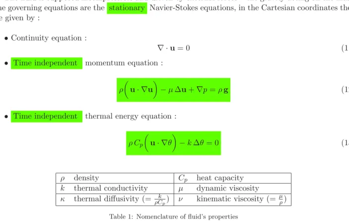
The fluid is supposed incompressible and driven by external forces – the gravity acting on the mass. The governing equations are the stationary Navier-Stokes equations, in the Cartesian coordinates they are given by :

• Continuity equation :

∇ · u = 0 (11)

• Time independent momentum equation : ρ

3

u_{· ∇u}

4

− µ ∆u + ∇p = ρ g (12)

• Time independent thermal energy equation : ρ Cp

3

u_{· ∇θ}

4

− k ∆θ = 0 (13)

ρ density Cp heat capacity

k thermal conductivity µ dynamic viscosity

κ thermal diffusivity (= _ρCk

p) ν kinematic viscosity (=

µ

ρ)

Table 1: Nomenclature of fluid’s properties

Considering a reference state in which the density ρref and the pressure pref are so that ∇pref = ρref g

and writing p = pref+ ˜p and ρ = ρref+ ˜ρ, equation (12) becomes

3 1 +_ρρ˜ ref 4 3 u_{· ∇u} 4 + 1

ρref∇˜p− νref ∆u =

˜ ρ

ρref g, with νref =

µ ρref

,

and equation (13) becomes 3

1 +_ρρ_ref˜

4 3

u_{· ∇θ}

4

− κref ∆θ = 0, with κref =

k ρrefCp

(9)

We place ourselves within the Boussinesq approximation7 _{for steady state, with} ˜

ρ= ρrefβ (θ − θref),

where β is the volumetric coefficient of the thermal expansion and θref some reference temperature

for which ρref = ρ, here we took θref = 295 Kelvin’s degrees. By applying this approximation, the

momentum equation (12) becomes :

u_{· ∇u +} 1

ρref∇˜

p_{− ν}ref ∆u = β(θ − θref) g, (14)

and the thermal energy equation (13) becomes

−κref∆θ + u · ∇θ = 0. (15)

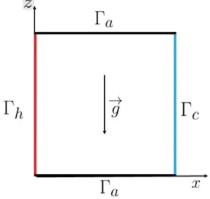
3.2. Application 1 : Natural convection in a 2D cavity

Figure 1: Geometry for a differentially heated square cavity

In this first example we investigate the case of a flow enclosed in a two-dimensional (x, z) differentially

heated square cavity (see Figure 1). The left wall is maintained at the hot temperature Th, the right

one at the cold temperature Tc = Tref whereas the walls at top and bottom are adiabatic.

The governing equations (11),(15) and (14) are made dimensionless by introducing ∆θ = Th − Tc

(the temperature difference), L (the distance between region of high temperature and region of low

temperature), the Grashof number Gr = gβ∆θL

2

ν2 (the ratio between the buoyant forces and viscous

forces acting on the fluid) and the Prandtl number P r = ν

κ (the ratio between the kinematic viscosity

and the thermal diffusivity). The following dimensionless quantities are introduced:

X = x L, Z = z L, U= u √ gβ∆θL, P = ˜ p gβ∆θLρref , Θ = θ− Tc Th− Tc 7

Boussinesq approximation states that the thermo-physical properties of the fluid (ρ, µ, Cp and k) are assumed to

be constant and independent of temperature except in the gravity term. Hence the variation of the density ρ˜ ρref

due to changes in the temperature can be neglected except in the gravity term.

(10)

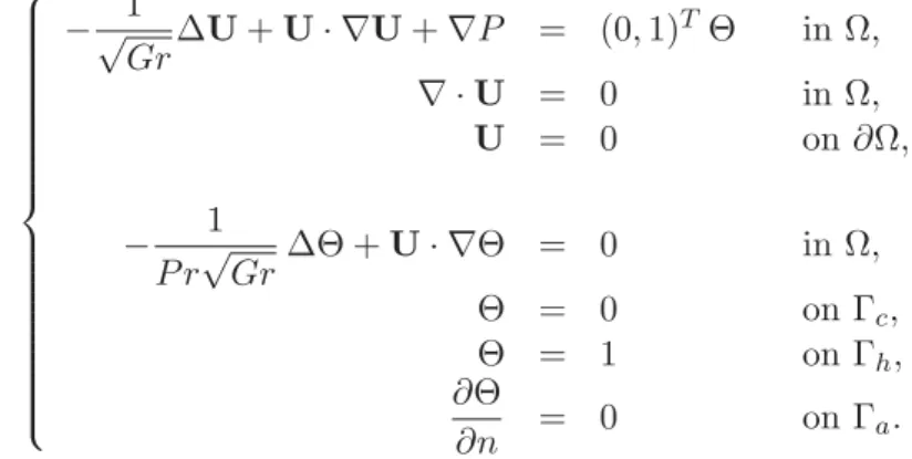
The dimensionless velocity U = (ux, uz), the dimensionless temperature θ, the pressure p of the fluid satisfy the following equations :

                                     −√1 Gr∆U + U · ∇U + ∇P = (0, 1) T _Θ _{in Ω,} ∇ · U = 0 in Ω, U = 0 on ∂Ω, − 1 P r√Gr∆Θ + U · ∇Θ = 0 in Ω, Θ = 0 on Γc, Θ = 1 on Γh, ∂Θ ∂n = 0 on Γa. (16)

The varying parameters of this example are the Grashof number Gr ∈ [103

,106

] and the Prandtl number

P r_{∈ [0.5, 1].}

3.3. Application 2 : Cooling system of electronic devices

In this second example we are interested by the variation of the temperature in a simplified system that is inspired by a suggested cooling system for electronic device (a small box with two electronic components).

(11)

The model is a two dimensional square where the cooling air enters the box at the Γin

b boundary and flows

around the two electronic components. Those two components produce heat energy at the boundary

Γout

c , and due to a convection phenomenon the heat energy is carried out by the fluid flow through the

box to finally exits from the boundary Γout

b (see Figure 2).

On the inflow section Γin

b a Poiseuille’s velocity profile vin = vb

A f(x)

0 B

is imposed, where vb is the

velocity magnitude and f (x) a parabolic function. On the outflow section Γout

b , homogenous Neumann

condition is imposed. For the flow passing through the electronic components, we have chosen to model

the interaction by non homogenous Dirichlet condition vc imposed to the second component of the

velocity on the inflow Γin

c and similarly on the outflow sections Γoutc .

We impose a temperature of θb on the inflow section Γinb and a temperature of θc on the outflow section

Γout

c , whereas the walls Γwall, the outflow section Γoutb and the inflow section Γinc are all adiabatic.

The velocity u = (ux, uz), the temperature θ, the pressure p of the fluid satisfy the following equations

: _                                                               ∇ · u = 0, u._{∇u +} 1 ρref∇˜

p_{− ν}ref∆u = β(θ − θref) g,

u_{· ∇θ − κ}ref ∆θ = 0, u = vin on Γinb ∂u ∂n = 0 on Γ out b u = 0 on Γwall uz = −vc, ux = 0 on Γoutc uz = −vc, ∂ux ∂n = 0 on Γ in c θ = θb on Γinb , θ = θc on Γoutc , ∂θ ∂n = 0 on ∂Ω \ {Γ out c ∪ Γinb }. (17)

The varying parameters are the velocities vb ∈ [0.5; 2], vc ∈ [0.1; 0.4] (in mm/s), the imposed

temperatures θb ∈ [288; 292] and θc ∈ [295; 315] (in Kelvin). For simplicity we will also denoted by

σ= (vb, θb, vc, θc) the set of parameters.

4. Numerical results

The blackbox software to compute the pressure, velocity and temperature “truth” and “coarse”

approximations is the finite element code “FreeFem++”[10]. The P2-P1 Taylor-Hood finite element has

been used to build the velocity and pressure approximation spaces and the P2 finite element has been

used to build the temperature approximation space over various coarse and fine meshes: TH and Th.

4.1. Application 1 : Natural convection in a 2D cavity

In this example, we consider heat transfer due to natural convection inside a heated cavity as introduced in section 3.2. To start with, we shall focus here on the approximation of the only temperature

θ, hence, in the remainder subsection, we have simplified the notation by removing the superscript θ on

(12)

In order to build the reduced basis space XN

h , we have computed a “training” sample made of a

series of ntrain = 93 fine finite element approximations of (16) for a Prandtl number varying between

0.5 and 1 and a Grashof number varying between 103

and 106

(see Figure 4).

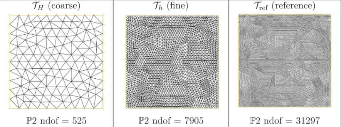
TH (coarse) Th (fine) Tref (reference)

P2 ndof = 525 P2 ndof = 7905 P2 ndof = 31297

Figure 3: Embedded meshes used to build finite element approximation spaces

1000 2000 3000 4000 6000 7000 8000 9000 10000 20000 30000 40000 60000 70000 80000 90000 100000 200000 300000 400000 600000 700000 800000 900000 0.5 0.6 0.8 1

Grashoff Number (log scale)

Prandtl Number

Figure 4: Parameters distribution in Ξtrain= [0.5 : 1] × [10

3

: 106

]

Let us denote by, ΞF

train, the “ full training” set of points, in D, associated to our complete “training”

sample of finite element approximations. In order to better take into account the disparity between the solutions of lower and higher Rayleigh number (Ra = Gr × P r), we have decomposed this initial

“training” parameter set into three parts (see figure 4) : ΞF

train = Ξ 1 train∪ Ξ 2 train∪ Ξ 3 train with                        ΞF train = [0.5 : 1] × [10 3 : 106 ], Ξ1 train = [0.5 : 1] × [10 3 : 104 ], Ξ2 train = [0.5 : 1] × [10 4 : 105 ], Ξ3 train = [0.5 : 1] × [10 5 : 106 ]. (18)

(13)

In order to obtain an optimal set of parameters {σ1,· · · , σ_N_max} from a given training sample Ξ_train⊂

ΞF_train, we resort to a greedy sampling procedure given in Algorithm 1.

Algorithm 1 _{Greedy’s algorithm used to choose {σ}1,· · · , σ_N_max}

Given Ξtrain = (σ1,· · · , σ_n_t) ∈ Dnt, n_t>>1 with n_t≤ n_train and Ξ_train ⊂ ΞF_train

Choose randomly σ1,→ S1 = {σ1} and X

1 h= span{θh(σ1)} Set ξ1 = θh(σ1) ëθh(σ1)ë_L2 forn= 2 to Nmax do σn= arg max σ∈Ξtrain ëθh(σ) − n−1 Ø i=1 (θh(σ), ξi)L2ξ_ië_L2 ëθh(σ)ëL2 Sn= Sn−1∪ σn and X_hk= X_hn−1+ span{θh(σn)} Compute ˜ξn= θh(σn) − n−1 Ø i=1 ξi(θh(σn), ξi)L2 and set ξ_n= ˜ ξn ë˜ξnëL2 end for

Besides, in order to determine the reduced basis’s optimal size we propose to look at the behavior of

the average error of the rectification process for all the σ ∈ Ξtrain\ SN as N increase to Nmax. In order

to do so, we computed temporary rectification matrices TN _{associated to the functionals {ξ}

i}1≤i≤N. To lighten the notation we introduce :

- The vectors Ti_{∈ R}N _{for i = 1, · · · , N defined by}

(Ti₎

j = TNi,j, ∀j = 1, · · · , N;

- The vectors Ai _{∈ R}N max _{for i = 1, · · · , N defined by}

(Ai₎

k= (θH(σk), ξi)L2 ∀k = 1, · · · , N_max;

- The vectors Bi _{∈ R}N max _{defined by}

(Bi₎

k= (θh(σk), ξi)L2, ∀k = 1, · · · , N_max;

- The matrix D ∈ RNmax×N _{defined by}

D=    A1 .. . AN   =    (θH(σ1), ξ1)_L2 · · · (θ_H(σ1), ξ_N)_L2 .. . ... ... (θH(σNmax), ξ1)L2 · · · (θH(σNmax), ξN)L2   .

In order to find the optimal coefficients TNij we resort to a least-square recipe with a penalty term. For

1 ≤ i ≤ N, we are looking for the vector TN

i which minimizes the following cost function Ci:

Ci _{= ëD T}i_{− B}i_ë22− λëTië

2

2 (19)

where λ is a regularization coefficient and ë · ë2 stand for the Euclidian ℓ2-norm. We can show that

minimization of the cost function(19) leads to a set of N linear equations in the N unknown coefficients

TNi,j and that it can be written as following the linear system:

(DT_D_{+ λ I}

(14)

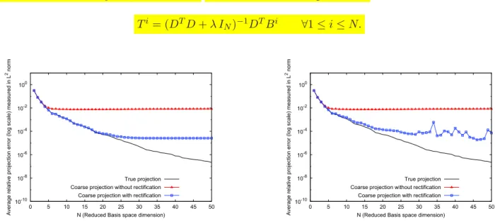
where IN is the identity matrix in RN ×N. The solution of this equation is : Ti= (DT_D_{+ λ I} N)−1DTBi ∀1 ≤ i ≤ N. 10-10 10-8 10-6 10-4 10-2 100 0 5 10 15 20 25 30 35 40 45 50 A

verage relative pro

jection error (log scale) measured in L

2 norm

N (Reduced Basis space dimension) True projection Coarse projection without rectification Coarse projection with rectification

10-10 10-8 10-6 10-4 10-2 100 0 5 10 15 20 25 30 35 40 45 50 A

verage relative pro

2 norm

Figure 5: Average errors with λ = 10−10 _{(left) and with λ = 0 (right) during the reduced basis construction stage with}

Ξtrain= ΞFtrain

Figure 5 shows for Ξtrain = ΞFtrain, the behavior of the rectification process with and without the

regu-larization. The average relative errors are measured in L2

-norm and defined by :

- for the true projection : 1

ntrain ntrain Ø k=1 . . . . θh(σk) − N Ø i=1 (θh(σk), ξi)L2ξ_i . . . . L2 ëθh(σk)ëL2 ,

- for the coarse projection without rectification : 1

ntrain ntrain Ø k=1 . . . . θh(σk) − N Ø i=1 (θH(σk), ξi)L2ξ_i . . . . L2 ëθh(σk)ëL2 ,

- for the coarse projection with rectification : 1

ntrain ntrain Ø k=1 . . . . θh(σk) − N Ø i,j=1 TNi,j(θH(σk), ξj)L2ξ_i . . . . L2 ëθh(σk)ëL2 . Without the regularization we observe peaks in the error curve due to a deterioration of the rectified solution when N is large.

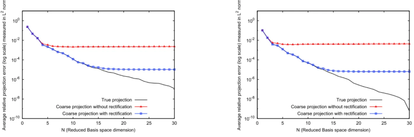
Figures 6 and 7 show for the different training sets introduced in (18), the behavior of the rectification

(15)

10-10 10-8 10-6 10-4 10-2 100 0 5 10 15 20 25 30 A

verage relative pro

2 norm

10-10 10-8 10-6 10-4 10-2 100 0 5 10 15 20 25 30 A

verage relative pro

2 norm

Figure 6: Average errors during the reduced basis construction stage with Ξtrain= Ξ

1

train∪ Ξ

2

train (left) and with

Ξtrain= Ξ 2 train(right) 10-10 10-8 10-6 10-4 10-2 100 0 5 10 15 20 25 30 A

verage relative pro

2 norm

10-10 10-8 10-6 10-4 10-2 100 0 5 10 15 20 25 30 A

verage relative pro

2 norm

Figure 7: Average errors during the reduced basis construction stage with Ξtrain= ΞFtrain\ Ξ

1

train(left) and Ξtrain= Ξ

3

train

(right)

With the regularization, the rectification process remains good when N is large, despite the fact that a threshold in the error is reached. Reminding that, as proven in [3, 4, 15], we have

ëθ(σ) − RNθH(σ) ëH1 ≤ c1(N )(h + H 2 ) + ε(N ), where RN θH(σ) = N Ø i,j=1

TNi,j(θH(σ), ξj)L2ξ_i. The behavior of the rectified solution R_Nθ_H(σ) observed

when N is large in figures 6 and 7 confirms that constant c1(N ) is growing with N .

Finally, we have decided to stop the enrichment of the reduced basis space when the rectification error stop decreasing rapidly and reach a threshold (see table 2).

(16)

Parameter space Ξtrain Nmax ΞF_train 30 Ξ1 train∪ Ξ 2 train 20 Ξ2 train 15 ΞF train\ Ξ 1 train 20 Ξ3 train 20 Table 2: Value of Nθ

maxfor a variety of Ξtrain

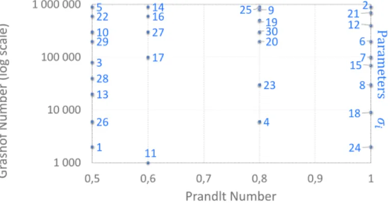
Figure 8, below shows the parameters distribution during the reduced basis construction stage with

Ξtrain= ΞFtrain. 1 2 3 4 5 6 7 8 9 10 11 12 13 14 15 16 17 18 19 20 21 22 23 24 25 26 27 28 29 30 1 000 10 000 100 000 1 000 000 0,5 0,6 0,7 0,8 0,9 1 Gr ashof Num ber (l og s cal e) Prandlt Number Param ete rs !

Figure 8: Parameters distribution during the reduced basis construction stage with Ξtrain= ΞFtrain

Once we have determined, for each parameter space Ξtrain, the set of parameters {σ1,· · · , σ_N_max} that

will be used to generate Xh

N, we solve, for several values of N ≤ Nmax, the following eigenvalue problem:

find (λk,Φk) ∈ RN × RN, 1 ≤ k ≤ N such that

KNΦk = λkMNΦk with MNi,j = Ú Ω ξiξj and KNi,j = Ú Ω∇ξi∇ξj .

Which will provide N basis functions of XN

h orthogonalized in L 2 and H1 norm, defined as φθ,N_k = _√1 λk N Ø i=1 (Φk)iξi.

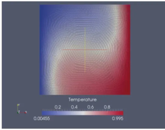
To validate the reduced basis functions, we have looked at the convergence rate of the H1

-orthogonal

projection from Xh into XhN for some particular solutions θh(σ), with σ ∈ D \ Ξtrain depending on the

parameters space Ξtrain. Figure 9 shows the temperature field θh(σ) with a lower Rayleigh number (on

(17)

Figure 9: Temperature field θh(σ) (on the left with σ = (0.75; 25 000) and on the right with σ = (0.7; 750 000))

Let the projection error measured in H1

-norm defined by ëΠNθh(σ) − θref(σ)ëH1 = . . . . N Ø i=1 (θh(σk), φθ,Ni )H1φθ,N i − θref(σ) . . . . H1 ëθref(σ)ëH1 ,

where θref(σ) is a reference FEM solution computed on the reference mesh Tref (see figure 3).

Figure 10 shows that the projection error is same as the fine FEM error for N = Nmax.

10−4 10−3 10−2 10−1 5 10 15 20 25 30 ëΠ N θh ( σ ) − θref ( σ )ëH 1 T em p er at u re re lat iv e er ror (l og sc al e)

N_{(Reduced Basis space dimension)}

FEM Error RB Projection error using ΞF

train

RB Projection error using Ξ1

train∪ Ξ

2

train

RB Projection error using ΞF

train\ Ξ 1 train 10−3 10−2 10−1 5 10 15 20 25 30 ëΠ N θh ( σ ) − θref ( σ )ëH 1 T em p er at u re re lat iv e er ror (l og sc al e)

N_{(Reduced Basis space dimension)}

FEM Error RB Projection error using ΞF

train

RB Projection error using ΞF

train\ Ξ

1

train

Figure 10: Convergence rate of the reduced basis’s projection measured in H1

-norm (on the left with σ = (0.75; 25 000) and on the right with σ = (0.7; 750 000))

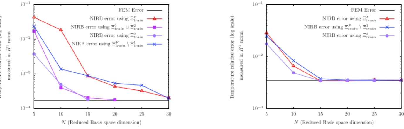
In the figure 11 we can see the convergence rate of the non-intrusive reduced basis (NIRB) approximation

θ_H,hN _{as function of N for some particular value of σ ∈ D \ Ξ}train depending on the parameters space

Ξtrain. We defined the relative NIRB error measured in H1-norm by

. . . . N Ø i,j=1 Rθ,N_i,j (θh(σk), φθ,Nj )L2φθ,N i − θref(σ) . . . . H1 ëθref(σ)ëH1 ,

(18)

10−4 10−3 10−2 10−1 5 10 15 20 25 30 T em p er at u re re lat iv e er ror (l og sc al e) m eas u re d in H 1n or m

N (Reduced Basis space dimension)

FEM Error NIRB error using ΞF

train

NIRB error using Ξ1

train∪ Ξ

2

train

NIRB error using ΞF

train\ Ξ 1 train 10−3 10−2 10−1 5 10 15 20 25 30 T em p er at u re re lat iv e er ror (l og sc al e) m eas u re d in H 1n or m

N (Reduced Basis space dimension)

FEM Error NIRB error using ΞF

train

NIRB error using ΞF

train\ Ξ

1

train

Figure 11: Convergence rate of the improved reduced basis approximation θN

H,h as function of N measured in H

1

-norm during the online stage (on the left with σ = (0.75; 25 000) and on the right with σ = (0.7; 750 000))

As we expected, we were able to reach the same accuracy as the fine finite element solution and to reduced significantly the computational times (see table 3).

F.E.M. NIRB method

Fine sol. (on line stage)

FEM Rectification

coarse sol. N=15 N=20 N=30

7min28 26 sec 5 sec 9 sec 19 sec

Table 3: Average execution’s times

4.2. Application 2 : Cooling system of electronic devices

In this second example, we are interested in the evaluation of the velocity and the temperature inside a simplified cooling system for electronics devices.

Th TH1 TH2 TH3

P2 Ndof = 20213 P2 Ndof = 5148 P2 Ndof = 5088 P2 Ndof = 1871

Figure 12: From the left to the right : fine mesh (Th), embedded coarse mesh (TH1), non embedded coarse mesh (TH2), non embedded very coarse mesh (TH3).

In order to build the reduced spaces XN

h and YhN we have used a fine finite element mesh with 20,213

(19)

computed a sample of coarse and fine finite element approximations of problem (17), using embedded

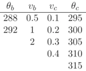
or non embedded meshes (see figure 12). The associated parameters space — denoted by Ξtrain — is of

size 120, and composed of parameters within the following values:

θb vb vc θc 288 0.5 0.1 295 292 1 0.2 300 2 0.3 305 0.4 310 315

To verify the non-intrusive reduced basis method, we have compared the fine finite element solution for

σ= (θb; vb; vc; θc) = (290; 1.5; 0.25; 312) (see figure 13) with different reduced solutions (see Figure 14).

(20)

10-4 10-3 10-2 10-1 Relative error in H 1-norm (log) N (log) Temperature 3 5 8 10 12 15 20 Case 1 Case 2 Case 3 Case 4 Case 2 + Rec Case 3 + Rec Case 4 + Rec 10-3 10-2 10-1 Relative error in H 1-norm (log) N (log) Velocity Case 1 Case 2 Case 3 Case 4 Case 2 + Rec Case 3 + Rec Case 4 + Rec

Figure 14: Relative error between the fine FEM solution and the various reduced solutions measured in H1

-norm (tem-perature on the left and velocity on the right).

• Case 1:

In this example, we want to see the error due only to the reduced basis size N . To do so, as in

the previous section, we have computed the L2

projection of the fine finite element solution on the reduced basis space.

For a given N , those solutions are the best approximation that we can expect in the reduced basis space.

• Case 2, 3 and 4:

In those examples, we wanted to see how the choice of the coarse mesh TH affect the NIRB method

when there is no rectification.

We have used embedded coarse mesh (TH = TH1) and not embedded coarse meshes (TH = TH2 or

TH3) to compute the reduced approximation in respectively the case 2, 3 and 4.

We notice that as N goes larger the error between the different reduced solutions and the FEM solution goes smaller to finally reach a threshold. This is due to the fact that the coarse finite element’s error become more significant than the reduced basis size’s error.

Remark : From a practical viewpoint, we want to use a finite element software able to compute

the coefficients γHi

j (σ) easily and in a way that it is not too time consuming. Indeed, in order

to do compute those coefficients we resort to numerical integration. However, in the case when the meshes are not embedded a supplementary difficulty arise from the fact that the reduced basis functions and the coarse solutions do not belong to a same finite element space. We want to avoid an extra interpolation error due to the interpolation of the coarse solution to the reference mesh.

It is made by the use of a numerical quadrature formula over each triangle Kh based Gauss points,

here we choose a P2-unisolvent formula (with 7 points). For example

Ú Kh θHi(σ)ξ j h will be replaced by 7 Ø p=1 ωp× θHi(xp; σ) × ξ j

h(xp), where ωp are the weight of the quadrature point. Then to compute

θHi(xp; σ), we just have to find in which triangle of THi belongs the point xp, to avoid any

inter-polation of θHi(σ) on Kh. In the software that we have used for our numerical experiments, this

(21)

• Case 2 + Rec, 3 + Rec and 4 + Rec : In those examples we wanted to see the influence of the rectification on the reduced solution. We observe that with this rectification we are able to reach the same accuracy as if we have projected the reference finite element solution on the reduced

basis space, even with the coarsest mesh. In particular, when using coarse mesh TH3, we are able

to divide the computational times by 10 without any loss of accuracy (see figures 15 and 16).

10-4 10-3 10-2

3 5 8 10 12 15 20

Temperature relative error in H

1-norm (log scale)

N

Two-grid FE/RB method convergence rate for σ = (1.5;290;0.25;305) and H = H3 depending on N

|| θh(σ) - PNθh(σ) ||H1 || θh(σ) - PNθH(σ) ||H1 || θh(σ) - RNPNθH(σ) ||H1 10-3 10-2 10-1 3 5 8 10 12 15 20

Velocity relative error in H

1-norm (log scale)

N

Two-grid FE/RB method convergence rate for = (1.5;290;0.25;305) and H = H depending on N

|| uh(σ) - PNuh(σ) ||H1 || u_h(σ) - P_Nu_H(σ) ||_H1

|| uh(σ) - RNPNuH(σ) ||H1

Figure 15: Relative error between the fine FEM solution the various reduced solutions measured in H1

-norm with TH= TH3 (temperature on the left and velocity on the right).

0.5 15 200 3 5 8 10 12 15 20 8 23

Times in seconds (log scale)

N

CPU Times of the two-grid FE/RB online stage for H = H depending on N

Total time

Rectification of θ_H

Computation of θ_H

Computation of θ_h

Figure 16: Comparison of CPU Times between the fine FEM and the NIRB method

4.3. Conclusion

The present paper illustrates the capability of non-intrusive reduced basis method to return compu-tationally efficient and accurate thermal flux for simple model of cooling systems. Coarse triangulations have been used to compute finite element solutions during the online stage. In order to regain accuracy,

(22)

we first project these solutions into the RB space, and then improve them via a rectification technique. Our numerical results prove that the two ingredients i) projection ii) rectification, are inseparable in order to get the expected accuracy. With this approach, we are still able to significantly reduce our computational cost without modifying the CFD code, and it is thus user-friendly. The only thing that we need to get out the plain CFD finite element software are: i) the meshes (fine and coarse) and ii) the nodal values of each fields we want to approximate, in order to export these data in a simple finite

element code (as e.g. Matlab, FEEL++, FreeFem++) where simple L2

and H1

scalar products are performed. Our simulations also illustrate that the coarse and fine meshes do not need to be embedded. Acknowledgment

The authors would like to graciously thank Pascal Joly for fruitful discussions and very valuable advice in the beginning of our project. This work was partially supported by the Research Grant FNRAE RB4FASTSIM.

5. References

[1] A. Buffa, Y. Maday, A.T Patera, C. Prud’homme and G. Turinici A priori convergence of the Greedy algorithm for the parametrized reduced basis method ESAIM: M2AN, 46 3 (2012) 595-603

[2] T. Chacón Rebollo, E. Delgado Ávila, M. Gómez Mármol, F. Ballarin, and G. Rozza, On a certified

Smagorinsky reduced basis turbulence model, SIAM Journal on Numerical Analysis (2017).

[3] R. Chakir and Y. Maday. Une méthode combinée d’éléments finis à deux grilles/bases réduites pour

l’approximation des solutions d’une E.D.P. param´etrique. C. R. Acad. Sci. Paris, Ser. I Vol 347, p435-440 (2009).

[4] R. Chakir and Y. Maday. A two-grid finite-element/reduced basis scheme for the approximation of the solution of parameter dependent P.D.E. Actes de congr`es du 9`eme colloque national en calcul des structures, Giens 2009.

[5] W.Chen, J. Hesthaven, B. Junqiang, Z. Yang and Y. Tihao, A greedy non-intrusive reduced order model for fluid dynamics American Institute of Aeronautics and Astronautics (2017)

[6] N.N. Cuong, N. Veroy and A.T. Patera, Certified real-time solution of parametrized partial differ-ential equations. Handbook of Materials Modeling, 1529-1564, (2005).

[7] S. Deparis. Reduced basis error bound computation fo parameter - dependant Navier-Stokes equa-tions by natural norm approach. SIAM J. Numer. Anal. Vol 46, p 2039-2067 (2008).

[8] S. Deparis and G. Rozza. Reduced basis method for multi-parameter-dependent steady Navier-Stokes equations: Applications to natural convection in a cavity. Journal of Computational Physics, Vol 228, No 12, p4359-4378 (2009).

[9] M. Grepl, Y. Maday, N. Nguyen, and A.T Patera. Efficient reduced-basis treatment of nonaffine and nonlinear partial differential equations, M2AN, Vol 41, No 3, p575-605 (2007).

[10] F. Hecht New development in FreeFem++. Journal of Numerical Mathematics, 20(3-4), pp. 251-266 (2012)

(23)

[11] J. Hesthaven, B. Stamm, S. Zhang,Efficient greedy algorithms for high-dimensional parameter spaces with applications to empirical interpolation and reduced basis methods, ESAIM-Math. Model. Num., Vol. 48, pp. 259-283 (2014)

[12] K. Ito and S.S. Ravindran. A reduced-order method for simulation and control of fluid flow. J. Computat. Phys., Vol 143, p403-425 (1998).

[13] A. Lovgren, Y. Maday and E. Ronquist . A reduced basis element method for the steady Stokes problem. ESAIM: Mathematical Modelling and Numerical Analysis, 40, pp 529-552, (2006). [14] Y. Maday. Reduced basis method for the rapid and reliable solution of partial differential equations.

in International Congress of Mathematicians, Vol. III, p1255-1270, Eur. Math. Soc. Zurich (2006). [15] O. Mula Quelques contributions vers la simulation parallèle de la cinétique neutronique et la prise en compte de données observées en temps réel. Phd thesis, Université Pierre et Marie Curie (2014). [16] J.S. Peterson. The reduced basis method for incompressible viscous flow calculations. SIAM Journal

on Scientific and Statistical Computing, Vol 10, No 4 p777-786 (1989).

[17] C. Prud’homme, D. Rovas, K. Veroy, L. Machiels, Y. Maday, A. Patera, and G. Turinici. Reli-able real-time solution of parametrized partial differential equations: Reduced-basis output bound methods. J Fluids Engineering, Vol 124 p70-80 (2002).

[18] A. Quarteroni and G. Rozza. Numerical Solution of Parametrized Navier-Stokes Equations by Re-duced Basis Methods Numer. Methods Partial Differential Equations, Vol 23, No 4, p923-948 (2007). [19] A. Quarteroni, G. Rozza, and A. Manzoni. Certified Reduced Basis Approximation for Parametrized Partial Differential Equations and Applications. Journal of Mathematics in Industry 2011 Vol 1, No 3 (2011).

[20] G. Rozza. Reduced Basis Approximation and Error Bounds for Potential Flows in Parametrized Geometries Commun. Comput. Phys. Vol 9, No 1, p1-48 (2011).

[21] G. Rozza, D.B.P Huynh, N.C. Nguyn and A.T. Patera Real-time reliable simulation of heat transfer phenomena, Proceeding of HT2009, ASME Summer Heat Transfer Conference (2009).

[22] G. Rozza and K. Veroy, On the stability of the reduced basis method for Stokes equations in parametrized domains, Computer Methods in Applied Mechanics and Engineering, Volume 196, Issue 7, 10, p1244-1260 (2007).

[23] G Pitton, A Quaini and G Rozza, Computational reduction strategies for the detection of steady bifurcations in incompressible fluid-dynamics: Applications to Coanda effect in cardiology Journal of Computational Physics, Volume 344, p534-557, (2017)

[24] E. Schenone, S. Veys and C. Prud’homme, High Performance Computing for the Reduced Basis Method. Application to Natural Convection. ESAIM: Proceedings, 43, p255-273. (2013).

[25] O. Souhar and C. Prud’homme, Numerical analysis method of heat transfer in an electronic com-ponent using sensitivity analysis. Journal of Computational Electronics. 13 (4), p1042-1053 (2014). [26] L. Fick, Y. Maday, A.T Patera and T. Taddei A Reduced Basis Technique for Long-Time Unsteady

(24)

[27] K. Veroy and A.T. Patera. Certified real-time solutions of the parametrized steady incompressible Navier-Stokes equations. International Journal for Numerical Methods in Fluids, Vol 47, p773-788 (2005).

[28] D. Xiao, F. Fang, A.G. Buchan, C.C. Pain, I.M. Navon, J. Du, G. Hu, , Non-linear model reduction for the Navier-Stokes equations using residual DEIM method, Journal of Computational Physics, Vol 263, p1-18 (2014).

[29] D. Xiao, F. Fang, C.C. Pain and I.M. Navon, A parameterized non-intrusive reduced order model and error analysis for general time-dependent nonlinear partial differential equations and its applications Computer Methods in Applied Mechanics and Engineering Vol 317, p868-889 (2017)