Measurement of $CP$-Averaged Observables in the $B^{0}\rightarrow K^{*0}\mu^{+}\mu^{-}$ Decay

(1)

EUROPEAN ORGANIZATION FOR NUCLEAR RESEARCH (CERN)

CERN-EP-2020-027 LHCb-PAPER-2020-002 July 15, 2020

Measurement

of CP -averaged observables

in the B

0

→ K

∗0

µ

+

µ

−

decay

LHCb collaboration† Abstract

An angular analysis of the B0 → K∗0_{(→ K}+_π−_)µ+_µ− _{decay is presented using a}

data set corresponding to an integrated luminosity of 4.7 fb−1 of pp collision data

collected with the LHCb experiment. The full set of CP -averaged observables are determined in bins of the invariant mass squared of the dimuon system.

Contamina-tion from decays with the K+π− system in an S-wave configuration is taken into

account. The tension seen between the previous LHCb results and the Standard Model predictions persists with the new data. The precise value of the significance of this tension depends on the choice of theory nuisance parameters.

Submitted to Phys. Rev. Lett.

(2)

(3)

Decays mediated by the quark-level transition b → s`+_`−_{, where ` represents a lepton,}

have been the subject of intense recent study, as angular observables [1–8], branching fractions [8–11] and ratios of branching fractions between decays with different flavours of leptons [12–16] have been measured to be in tension with Standard Model (SM) predictions. Such decays are suppressed in the SM, as they proceed only through amplitudes that involve electroweak loop diagrams. The decays are sensitive to virtual contributions from new particles, which could have masses that are inaccessible to direct searches. The observed anomalies with respect to SM predictions can be explained consistently in New Physics models that introduce an additional vector or axial-vector contribution [17–35]. However, there is still considerable debate about whether some of the observations might instead be explained by hadronic uncertainties associated with the transition form factors, or by other long-distance effects [36–39].

The LHCb collaboration presented a measurement of the angular observables of the B0_{→ K}∗0_µ+_µ−_{decay in Ref. [1] and found that the data could be explained by modifying}

the real part of the vector coupling strength of the decays, conventionally denoted Re(C9).

The analysis used the nuisance parameters from Ref. [40], implemented in the EOS software package described in Ref. [41], and found a 3.4 standard deviation (σ) tension with the SM value of Re(C9). The tension observed depends on the values of various SM

nuisance parameters, including form-factor parameters and subleading corrections used to account for long-distance QCD interference effects with the charmonium modes. Using the Flavio software package [42], with its default SM nuisance parameters, gives a tension of 3.0 σ with respect to the SM value of Re(C9) when fitting the angular observables

from Ref. [1]. The nuisance parameters include a recent treatment of the subleading corrections [43, 44] that was not available at the time of the previous analysis.

This letter presents the most precise measurements of the complete set of CP -averaged angular observables in the decay B0 _{→ K}∗0_µ+_µ−_{. The data set corresponds to an}

integrated luminosity of 4.7 fb−1 of pp collisions collected with the LHCb experiment. The data were taken in the years 2011, 2012 and 2016, at centre-of-mass energies of 7, 8 and 13 TeV, respectively. The analysis uses the same technique as the analysis described in Ref. [1] but the data sample contains approximately twice as many B0 _{decays, owing}

to the addition of the 2016 data. The bb production cross-section increases by roughly a factor of two between the Run 1 and 2016 datasets [45]. The same 2011 and 2012 (Run 1) data as in Ref. [1] are used in the present analysis. The results presented in this letter supersede the previous LHCb publication. The combination of the Run 1 data set with the 2016 data set requires a simultaneous angular fit to account for efficiency and reconstruction differences between years. Throughout this letter, K∗0 is used to refer to the K∗(892)0 resonance and the inclusion of charge-conjugate processes is implied. The K∗0 meson is reconstructed through the decay K∗0→ K+_π−_.

The final state of the B0_{→ K}∗0_µ+_µ− _{decay can be described by the invariant mass}

squared of the dimuon system, q2, the invariant mass of the K+π− system, and the three decay angles, ~Ω = (cos θ, cos θ , φ). The angle between the µ+ _(µ−_{) and the direction}

(4)

of the B0_{→ K}∗0_µ+_µ− _{decay with the K}+_π− _{system in a P-wave configuration can be} written as 1 d(Γ + ¯Γ)/dq2 d4_{(Γ + ¯}_Γ) dq2_d~_Ω P = 9 32π h 3 4(1 − FL) sin 2_θ K+ FLcos2θK +1₄(1 − FL) sin2θKcos 2θl

−FLcos2θKcos 2θl+ S3sin2θKsin2θlcos 2φ

+S4sin 2θKsin 2θlcos φ + S5sin 2θKsin θlcos φ

+4₃AFBsin2θKcos θl+ S7sin 2θKsin θlsin φ

+S8sin 2θKsin 2θlsin φ + S9sin2θKsin2θlsin 2φ

i ,

(1)

where FL is the fraction of the longitudinal polarisation of the K∗0 meson, AFB is

the forward-backward asymmetry of the dimuon system and Si are other CP -averaged

observables [1]. The K+_π− _{system can also be in an S-wave configuration, which modifies}

the angular distribution to

1 d(Γ + ¯Γ)/dq2 d4_{(Γ + ¯}_Γ) dq2_d~_Ω S+P = (1 − FS) 1 d(Γ + ¯Γ)/dq2 d4_{(Γ + ¯}_Γ) dq2_d~_Ω P + 3 16πFSsin 2_θ l + 9 32π(S11+ S13cos 2θl) cos θK + 9

32π(S14sin 2θl+ S15sin θl) sin θKcos φ

+ 9

32π(S16sin θl+ S17sin 2θl) sin θKsin φ , (2)

where FS denotes the S-wave fraction and the coefficients S11, S13–S17 arise from

in-terference between the S- and P-wave amplitudes. Throughout this letter, FS and the

interference terms between the S- and P-wave are treated as nuisance parameters. Additional sets of observables, for which the leading B0 _{→ K}∗0 _form-factor

uncertain-ties cancel, can be built from FL, AFB and S3–S9. Examples of such optimised observables

include the P_i(0) series of observables [48]. The notation used in this letter again follows Ref. [1], for example P₅0 = S5/pFL(1 − FL).

The LHCb detector is a single-arm forward spectrometer covering the pseudorapidity range 2 < η < 5, described in detail in Refs. [49, 50]. The detector includes a vertex detector surrounding the proton-proton interaction region, tracking stations on either side of a dipole magnet, ring-imaging Cherenkov (RICH) detectors, electromagnetic and

(5)

Similarly, the simulated particle identification (PID) performance is corrected to match that determined from control samples selected from the data [57, 58].

The online event selection is performed by a trigger, which comprises a hardware stage, based on information from the calorimeter and muon systems, followed by a software stage that applies a full event reconstruction [59]. Offline, signal candidates are formed from a pair of oppositely charged tracks that are identified as muons, combined with a K∗0 candidate.

The distribution of the reconstructed K+_π−_µ+_µ− _{invariant mass, m(K}+_π−_µ+_µ−_{), is}

used to discriminate signal from background. This distribution is fitted simultaneously with the three decay angles. The distribution of the reconstructed K+π− mass, m(K+π−), depends on the K+_π− _{angular-momentum configuration and is used to constrain the}

S-wave fraction. The analysis procedure is cross-checked by performing a fit of the b → ccs tree-level decay B0→ J/ψK∗0, with J/ψ → µ+µ−, which results in the same final-state particles. Hereafter, the B0_{→ J/ψ(→ µ}+_µ−_)K∗0 _{decay and the equivalent decay via the}

ψ(2S) resonance are denoted by B0→ J/ψK∗0 _{and B}0_{→ ψ(2S)K}∗0_{, respectively.}

Two types of backgrounds are considered: combinatorial background, where the selected particles do not originate from a single b-hadron decay; and peaking backgrounds, where a single decay is selected but with some of the final-state particles misidentified. The combinatorial background is distributed smoothly in m(K+π−µ+µ−), whereas the peaking backgrounds can accumulate in specific regions of the reconstructed mass. In addition, the decays B0_{→ J/ψK}∗0_{, B}0_{→ ψ(2S)K}∗0 _{and B}0_{→ φ(1020)(→ µ}+_µ−_)K∗0 _{are removed by}

rejecting events with q2 in the ranges 8.0 < q2 < 11.0 GeV2/c4, 12.5 < q2 < 15.0 GeV2/c4 or 0.98 < q2 _{< 1.10 GeV}2_/c4_.

The criteria used to select candidates from the Run 1 data are the same as those described in Ref. [1]. The selection of the 2016 data follows closely that of the Run 1 data. Candidates are required to have 5170 < m(K+_π−_µ+_µ−_{) < 5700 MeV/c}2

and 795.9 < m(K+_π−_{) < 995.9 MeV/c}2_{. The four tracks of the final-state particles are}

required to have significant impact parameter (IP) with respect to all primary vertices (PVs) in the event. The tracks are fitted to a common vertex, which is required to be of good quality. The IP of the B0 _{candidate is required to be small with respect to one of}

the PVs. The vertex of the B0 candidate is required to be significantly displaced from the same PV. The angle between the reconstructed B0 _{momentum and the vector connecting}

this PV to the reconstructed B0 _{decay vertex, θ}

DIRA, is also required to be small. To

avoid the same track being used to construct more than one of the final state particles, the opening angle between every pair of tracks is required to be larger than 1 mrad.

Combinatorial background is reduced further using a boosted decision tree (BDT) algorithm [60, 61]. The BDT is trained entirely on data with B0 → J/ψK∗0

candi-dates used as a proxy for the signal and candicandi-dates from the upper-mass sideband 5350 < m(K+_π−_µ+_µ−_{) < 7000 MeV/c}2 _{used as a proxy for the background. The training}

uses a cross-validation technique [62] and is performed separately for the Run 1 and 2016 data sets. The input variables used are the reconstructed B0 _{decay-time and vertex-fit}

(6)

signal. The signal efficiency of the BDT is uniform in the m(K+_π−_µ+_µ−_{) and m(K}+_π−₎

distributions.

Peaking backgrounds from B_s0 → φ(1020)(→ K+_K−_)µ+_µ−_{, Λ}0

b → pK

−_µ+_µ−_,

B0_{→ J/ψK}∗0_{, B}0_{→ ψ(2S)K}∗0 _{and B}0_{→ K}∗0_µ+_µ− _{decays are considered, where the}

latter constitutes a background if the kaon from the K∗0 decay is misidentified as the pion and vice versa. In each case, at least one particle needs to be misidentified for the decay to be reconstructed as a signal candidate. Vetoes to reduce these peaking backgrounds are formed by placing requirements on the invariant mass of the candidates, recomputed with the relevant change in the particle mass hypotheses, and by using PID information. In addition, in order to avoid having a strongly peaking contribution to the cos θK angular distribution in the upper mass sideband, B+→ K+µ+µ− candidates with

K+µ+µ− invariant mass within 60 MeV/c2 of the B+ mass are removed. The background from b-hadron decays with two hadrons misidentified as muons is negligible. The signal efficiency and residual peaking backgrounds are estimated using simulated events. The vetoes remove a negligible amount of signal. The largest residual backgrounds are from B0→ K∗0µ+µ−, Λ0_b→ pK−µ+µ− and B_s0→ φ(1020)(→ K+_K−

)µ+µ− decays, at the level of 1% or less of the expected signal yield. This is sufficiently small such that these backgrounds are neglected in the angular analysis and are considered only as sources of systematic uncertainty.

For every q2 _{bin, a fit is performed in both the standard and the optimised basis.}

For each basis, four data sets are fit simultaneously: the m(K+_π−_µ+_µ−_{) and angular}

distributions of candidates in the Run 1 data; the equivalent distributions for the 2016 data; and the m(K+_π−_{) distributions of candidates in the Run 1 and the 2016 data sets.}

The signal fraction is shared between the two data sets from each data-taking period. The CP -averaged angular observables and the S-wave fraction are shared between all data sets. The fitted probability density functions (PDFs) are of an identical form to those of Ref. [1], as are the q2 _{bins used. In addition to the narrow q}2 _{bins, results are obtained}

for the wider bins 1.1 < q2 < 6.0 GeV2/c4 and 15.0 < q2 < 19.0 GeV2/c4.

The angular distribution of the signal is described using Eq. (1). The P_i(0) observables are determined by reparameterising Eq. (1) using a basis comprising F_L, P_1,2,3 and P_4,5,6,80 . The angular distribution is multiplied by an acceptance model used to account for the effect of the reconstruction and candidate selection. The acceptance function is parameterised in four dimensions, according to

ε(cos θl, cos θK, φ, q2) =

X

ijmn

cijmnLi(cos θl)Lj(cos θK)Lm(φ)Ln(q2) , (3)

where the terms Lh(x) denote Legendre polynomials of order h and the values of the

angles and q2 _{are rescaled to the range −1 < x < +1 when evaluating the polynomials.}

For the cos θl, cos θK and φ angles, the sum in Eq. (3) encompasses Lh(x) up to fourth,

(7)

value of q2 _{fixed at the bin centre. In the wider q}2 _{bins, the shape of the acceptance can}

vary significantly across the bin. In the likelihood, candidates are therefore weighted by the inverse of the acceptance function and parameter uncertainties are obtained using a bootstrapping technique [64].

The background angular distribution is modelled with second-order polynomials in cos θl, cos θK and φ, with the angular coefficients allowed to vary in the fit. This angular

distribution is assumed to factorise in the three decay angles, which is confirmed to be the case for candidates in the upper mass sideband of the data.

The m(K+π−µ+µ−) distribution of the signal candidates is modelled using the sum of two Gaussian functions with a common mean, each with a power-law tail on the low mass side. The parameters describing the signal mass shape are determined from a fit to the B0→ J/ψK∗0 _{decay in the data and are subsequently fixed when fitting}

the B0→ K∗0µ+µ− candidates. For each of the q2 bins, a scale factor that is deter-mined from simulation is included to account for the difference in resolution between the B0→ J/ψK∗0 _{and B}0_{→ K}∗0_µ+_µ− _{decay modes. A component is included in the}

B0→ J/ψK∗0 fit to account for B0_s→ J/ψK∗0 decays, which are at the level of ∼ 1% of the B0_{→ J/ψK}∗0 _{signal yield. The background from the equivalent Cabibbo-suppressed}

penguin decay, B0_s→ K∗0_µ+_µ− _{[65], is negligible and is ignored in the fit of the signal}

decay. The combinatorial background is described well by an exponential distribution in m(K+_π−_µ+_µ−_).

The K∗0signal component in the m(K+_π−_{) distribution is modelled using a relativistic}

Breit-Wigner function for the P-wave component and the LASS parameterisation [66] for the S-wave component. The combinatorial background is described by a linear function in m(K+_π−_).

The decay B0→ J/ψK∗0 _{is used to cross-check the analysis procedure in the region}

8.0 < q2 _{< 11.0 GeV}2_/c4_{. This decay is selected in the data with negligible background}

contamination. The angular structure has been determined by measurements made by the BaBar, Belle and LHCb collaborations [67–69]. The B0→ J/ψK∗0 _{angular observables}

obtained from the Run 1 and 2016 LHCb data, using the acceptance correction derived as described above, are in good agreement with these previous measurements.

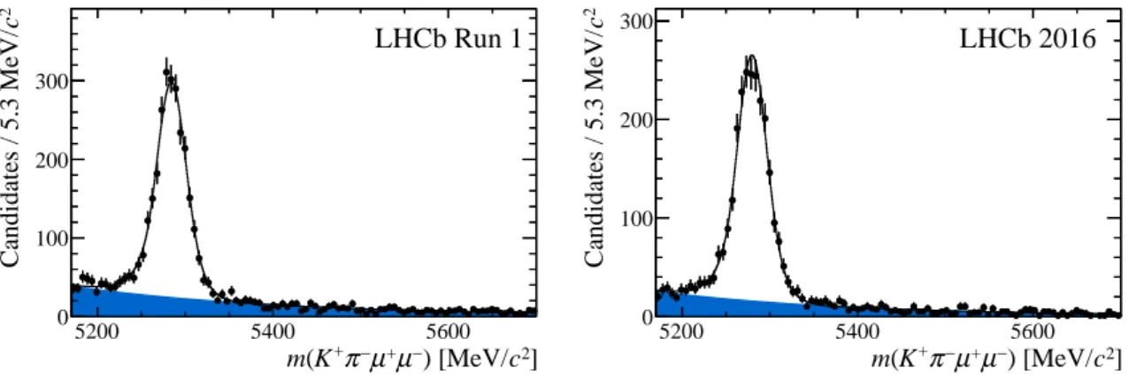
Figure 1 shows the projection of the fitted PDF on the K+π−µ+µ− mass distribu-tion. The B0_{→ K}∗0_µ+_µ− _{yield, integrated over the q}2 _{ranges 0.10 < q}2 _{< 0.98 GeV}2_/c4_,

1.1 < q2 _{< 8.0 GeV}2_/c4_{, 11.0 < q}2 _{< 12.5 GeV}2_/c4 _{and 15.0 < q}2 _{< 19.0 GeV}2_/c4_{, is}

deter-mined to be 2398 ± 57 for the Run 1 data, and 2187 ± 53 for the 2016 data.

Pseudoexperiments, generated using the results of the best fit to data, are used to assess the bias and coverage of the fit. The majority of observables have a bias of less than 10% of their statistical uncertainty, with the largest bias being 17%, and all observables have an uncertainty estimate within 10% of the true uncertainty. The biases are driven by boundary effects in the observables. The largest effect comes from requiring that FS ≥ 0, which can bias FS to larger values. This can then result in a bias in the P-wave

(8)

under-5200 5400 5600 ] 2 c ) [MeV/ − µ + µ − π + K ( m 0 100 200 300 2_c Candidates / 5.3 MeV/ LHCb Run 1 5200 5400 5600 ] 2 c ) [MeV/ − µ + µ − π + K ( m 0 100 200 300 2_c Candidates / 5.3 MeV/ LHCb 2016

Figure 1: The K+_π−_µ+_µ− _{mass distribution of candidates with 0.1 < q}2 _{< 19.0 GeV}2_/c4_,

excluding the φ(1020) and charmonium regions, for the (left) Run 1 data and (right) 2016 data. The background is indicated by the shaded region.

signal yields many times larger than the data, in order to render statistical fluctuations negligible.

The size of the total systematic uncertainty varies depending on the angular observable and the q2 bin. The majority of observables in both the Si and P

(0)

i basis have a total

systematic uncertainty between 5% and 25% of the statistical uncertainty. For FL, the

systematic uncertainty tends to be larger, typically between 20% and 50%. The systematic uncertainties are given in Table 3 of the Supplemental Material.

The dominant systematic uncertainties arise from the peaking backgrounds that are neglected in the analysis, the bias correction, and, for the narrow q2 _{bins, from the}

uncertainty associated with evaluating the acceptance at a fixed point in q2. For the peaking backgrounds, the systematic uncertainty is evaluated by injecting additional candidates, drawn from the angular distributions of the background modes, into the pseudoexperiment data. The systematic uncertainty for the bias correction is determined directly from the pseudoexperiments used to validate the fit. The systematic uncertainty from the variation of the acceptance with q2 _{is determined by moving the point in q}2 _at

which the acceptance is evaluated to halfway between the bin centre and the upper or the lower edge. The largest deviation is taken as the systematic uncertainty. Examples of further sources of systematic uncertainty investigated include the m(K+_π−_{) lineshape}

for the S-wave contribution, the assumption that the acceptance function is flat across the m(K+_π−_{) mass, the effect of the B}+_{→ K}+_µ+_µ− _{veto on the angular distribution of}

the background and the order of polynomial used for the background parameterisation. These sources make a negligible contribution to the total uncertainty. With respect to the analysis of Ref. [1], the systematic uncertainty from residual differences between data and simulation is significantly reduced, owing to an improved decay model for B0_{→ J/ψK}∗0

(9)

0 5 10 15 ] 4 c / 2 [GeV 2 q 0 0.2 0.4 0.6 0.8 1 L F (1S) ψ / J (2S)ψ LHCb Run 1 + 2016 SM from ASZB 0 5 10 15 ] 4 c / 2 [GeV 2 q 0.5 − 0 0.5 FB A (1S) ψ / J (2S)ψ LHCb Run 1 + 2016 SM from ASZB 0 5 10 15 ] 4 c / 2 [GeV 2 q 0.5 − 0 0.5 5 S (1S) ψ / J (2S)ψ LHCb Run 1 + 2016 SM from ASZB 0 5 10 15 ] 4 c / 2 [GeV 2 q 1 − 0.5 − 0 0.5 1 5 ' P (1S) ψ / J (2S)ψ LHCb Run 1 + 2016 SM from DHMV

Figure 2: Results for the CP -averaged angular observables FL, AFB, S5 and P50 in bins of q2.

The data are compared to SM predictions based on the prescription of Refs. [43, 44], with the

exception of the P₅0 distribution, which is compared to SM predictions based on Refs. [70, 71].

q2 [72, 73] to yield more precise determinations of the form factors over the full q2 range. For the P_i(0) observables, predictions from Ref. [70] are shown using form factors from Ref. [71]. These predictions are restricted to the region q2 < 8.0 GeV2/c4. The results from Run 1 and the 2016 data are in excellent agreement. A stand-alone fit to the Run 1 data reproduces exactly the central values of the observables obtained in Ref. [1].

Considering the observables individually, the results are largely in agreement with the SM predictions. The local discrepancy in the P₅0 observable in the 4.0 < q2 _{< 6.0 GeV}2_/c4

and 6.0 < q2 _{< 8.0 GeV}2_/c4 _{bins reduces from the 2.8 and 3.0 σ observed in Ref. [1] to 2.5}

and 2.9 σ. However, as discussed below, the overall tension with the SM is observed to increase mildly.

Using the Flavio software package [42], a fit of the angular observables is performed varying the parameter Re(C9). The default Flavio SM nuisance parameters are used,

including form-factor parameters and subleading corrections to account for long-distance QCD interference effects with the charmonium decay modes [43, 44]. The same q2 _{bins as}

(10)

using the observables from Ref. [1] and 2.7 σ tension with the measurements reported here.

In summary, using 4.7 fb−1 of pp collision data collected with the LHCb experiment during the years 2011, 2012 and 2016, a complete set of CP -averaged angular observables has been measured for the B0_{→ K}∗0_µ+_µ−_{decay. These are the most precise measurements}

of these quantities to date.

Acknowledgements

We express our gratitude to our colleagues in the CERN accelerator departments for the excellent performance of the LHC. We thank the technical and administrative staff at the LHCb institutes. We acknowledge support from CERN and from the national agencies: CAPES, CNPq, FAPERJ and FINEP (Brazil); MOST and NSFC (China); CNRS/IN2P3 (France); BMBF, DFG and MPG (Germany); INFN (Italy); NWO (Netherlands); MNiSW and NCN (Poland); MEN/IFA (Romania); MSHE (Russia); MinECo (Spain); SNSF and SER (Switzerland); NASU (Ukraine); STFC (United Kingdom); DOE NP and NSF (USA). We acknowledge the computing resources that are provided by CERN, IN2P3 (France), KIT and DESY (Germany), INFN (Italy), SURF (Netherlands), PIC (Spain), GridPP (United Kingdom), RRCKI and Yandex LLC (Russia), CSCS (Switzerland), IFIN-HH (Romania), CBPF (Brazil), PL-GRID (Poland) and OSC (USA). We are indebted to the communities behind the multiple open-source software packages on which we depend. Individual groups or members have received support from AvH Foundation (Germany); EPLANET, Marie Sk lodowska-Curie Actions and ERC (European Union); ANR, Labex P2IO and OCEVU, and R´egion Auvergne-Rhˆone-Alpes (France); Key Research Program of Frontier Sciences of CAS, CAS PIFI, and the Thousand Talents Program (China); RFBR, RSF and Yandex LLC (Russia); GVA, XuntaGal and GENCAT (Spain); the Royal Society and the Leverhulme Trust (United Kingdom).

(11)

Supplemental Material

This supplemental material includes additional information to that already provided in the main letter. A full set of results for the nominal analysis is presented in both graphical and tabular form in Sec. 1. A complete description of the corresponding systematic uncertainties is given in Sec. 2. The correlations between the angular observables are presented for the Si observables in Sec. 3 and for the P

(0)

i observables in Sec. 4. The

angular and mass distributions of the selected candidates in the different q2 _{bins are shown}

in Sec. 5.

1 Results

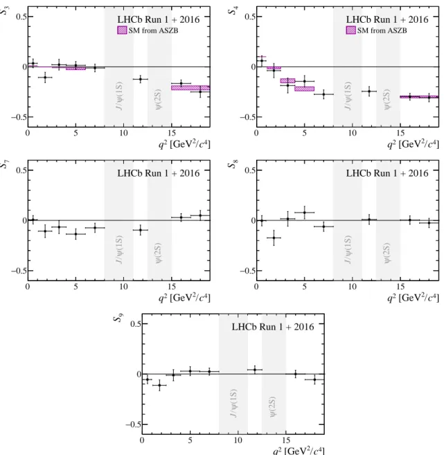
The values of S3, S4 and S7–S9 obtained from the simultaneous fit are shown in Fig. 3. The

data are compared to theoretical predictions based on the prescription of Ref. [44]. The predictions combine light-cone sum rule calculations [43] with lattice determinations [72,73] of the B0 → K∗0_{form factors. Figure 4 shows the values of the optimised observables, P}(0)

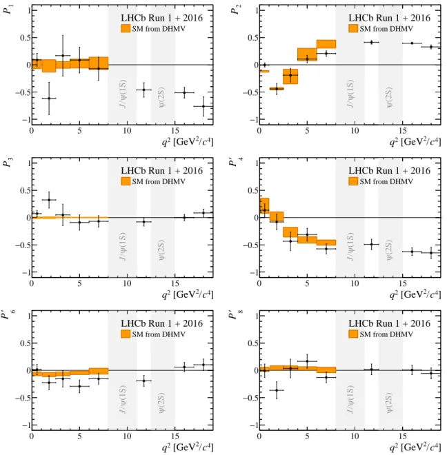
i ,

obtained from the fit. The data are compared to predictions based on the prescription in Ref. [70]. These predictions use form factors from Ref. [71]. The values of the observables in the standard and optimised basis are given in Tables 1 and 2, respectively. The statistical correlation between the observables in each q2 _{bin is provided in Tables 4–13}

(12)

0 5 10 15 ] 4 c / 2 [GeV 2 q 0.5 − 0 0.5 3 S (1S) ψ / J (2S)ψ LHCb Run 1 + 2016 SM from ASZB 0 5 10 15 ] 4 c / 2 [GeV 2 q 0.5 − 0 0.5 4 S (1S) ψ / J (2S)ψ LHCb Run 1 + 2016 SM from ASZB 0 5 10 15 ] 4 c / 2 [GeV 2 q 0.5 − 0 0.5 7 S (1S) ψ / J (2S)ψ LHCb Run 1 + 2016 0 5 10 15 ] 4 c / 2 [GeV 2 q 0.5 − 0 0.5 8 S (1S) ψ / J (2S)ψ LHCb Run 1 + 2016 0 5 10 15 ] 4 c / 2 [GeV 2 q 0.5 − 0 0.5 9 S (1S) ψ / J (2S)ψ LHCb Run 1 + 2016

Figure 3: Results for the CP -averaged angular observables S3, S4 and S7–S9 in bins of q2. The

(13)

0 5 10 15 ] 4 c / 2 [GeV 2 q 1 − 0.5 − 0 0.5 1 1 P (1S) ψ / J (2S)ψ LHCb Run 1 + 2016 SM from DHMV 0 5 10 15 ] 4 c / 2 [GeV 2 q 1 − 0.5 − 0 0.5 1 2 P (1S) ψ / J (2S)ψ LHCb Run 1 + 2016 SM from DHMV 0 5 10 15 ] 4 c / 2 [GeV 2 q 1 − 0.5 − 0 0.5 1 3 P (1S) ψ / J (2S)ψ LHCb Run 1 + 2016 SM from DHMV 0 5 10 15 ] 4 c / 2 [GeV 2 q 1 − 0.5 − 0 0.5 1 4 ' P (1S) ψ / J (2S)ψ LHCb Run 1 + 2016 SM from DHMV 0 5 10 15 ] 4 c / 2 [GeV 2 q 1 − 0.5 − 0 0.5 1 6 ' P (1S) ψ / J (2S)ψ LHCb Run 1 + 2016 SM from DHMV 0 5 10 15 ] 4 c / 2 [GeV 2 q 1 − 0.5 − 0 0.5 1 8 ' P (1S) ψ / J (2S)ψ LHCb Run 1 + 2016 SM from DHMV

Figure 4: Results for the optimised angular observables P1–P3, P40, P60 and P80 in bins of q2. The

(14)

Table 1: Results for the CP -averaged observables FL, AFB and S3–S9. The first uncertainties

are statistical and the second systematic.

0.10 < q2< 0.98 GeV2/c4 FL 0.255 ± 0.032 ± 0.007 S3 0.034 ± 0.044 ± 0.003 S4 0.059 ± 0.050 ± 0.004 S5 0.227 ± 0.041 ± 0.008 AFB −0.004 ± 0.040 ± 0.004 S7 0.006 ± 0.042 ± 0.002 S8 −0.003 ± 0.051 ± 0.001 S9 −0.055 ± 0.041 ± 0.002 1.1 < q2< 2.5 GeV2/c4 FL 0.655 ± 0.046 ± 0.017 S3 −0.107 ± 0.052 ± 0.003 S4 −0.038 ± 0.070 ± 0.011 S5 0.174 ± 0.060 ± 0.007 AFB −0.229 ± 0.046 ± 0.009 S7 −0.107 ± 0.063 ± 0.004 S8 −0.174 ± 0.075 ± 0.002 S9 −0.112 ± 0.054 ± 0.005 2.5 < q2< 4.0 GeV2/c4 FL 0.756 ± 0.047 ± 0.023 S3 0.020 ± 0.053 ± 0.002 S4 −0.187 ± 0.074 ± 0.008 S5 −0.064 ± 0.068 ± 0.010 AFB −0.070 ± 0.043 ± 0.006 S7 −0.066 ± 0.065 ± 0.004 S8 0.016 ± 0.074 ± 0.002 S9 −0.012 ± 0.055 ± 0.003 4.0 < q2_{< 6.0 GeV}2 /c4 FL 0.684 ± 0.035 ± 0.015 S3 0.014 ± 0.038 ± 0.003 S4 −0.145 ± 0.057 ± 0.004 S5 −0.204 ± 0.051 ± 0.013 AFB 0.050 ± 0.033 ± 0.002 S7 −0.136 ± 0.053 ± 0.002 S8 0.077 ± 0.062 ± 0.001 S9 0.029 ± 0.045 ± 0.002 6.0 < q2_{< 8.0 GeV}2 /c4 FL 0.645 ± 0.030 ± 0.011 S3 −0.013 ± 0.038 ± 0.004 S4 −0.275 ± 0.045 ± 0.006 S5 −0.279 ± 0.043 ± 0.013 AFB 0.110 ± 0.027 ± 0.005 S7 −0.074 ± 0.046 ± 0.003 S8 −0.062 ± 0.047 ± 0.001 S9 0.024 ± 0.035 ± 0.002 11.0 < q2_{< 12.5 GeV}2 /c4 FL 0.461 ± 0.031 ± 0.010 S3 −0.124 ± 0.037 ± 0.003 S4 −0.245 ± 0.047 ± 0.007 S5 −0.310 ± 0.043 ± 0.011 AFB 0.333 ± 0.030 ± 0.008 S7 −0.096 ± 0.050 ± 0.003 S8 0.009 ± 0.049 ± 0.001 S9 0.042 ± 0.040 ± 0.003 15.0 < q2_{< 17.0 GeV}2_/c4 FL 0.352 ± 0.026 ± 0.009 S3 −0.166 ± 0.034 ± 0.007 S4 −0.299 ± 0.033 ± 0.008 S5 −0.341 ± 0.034 ± 0.009 AFB 0.385 ± 0.024 ± 0.007 S7 0.029 ± 0.039 ± 0.001 S8 0.003 ± 0.042 ± 0.002 S9 0.000 ± 0.037 ± 0.002 17.0 < q2_{< 19.0 GeV}2_/c4 FL 0.344 ± 0.032 ± 0.025 S3 −0.250 ± 0.050 ± 0.025 S4 −0.307 ± 0.041 ± 0.008 S5 −0.280 ± 0.040 ± 0.014 AFB 0.323 ± 0.032 ± 0.019 S7 0.049 ± 0.049 ± 0.007 S8 −0.026 ± 0.046 ± 0.002 S9 −0.056 ± 0.045 ± 0.002 1.1 < q2_{< 6.0 GeV}2_/c4 FL 0.700 ± 0.025 ± 0.013 S3 −0.012 ± 0.025 ± 0.003 S4 −0.136 ± 0.039 ± 0.003 S5 −0.052 ± 0.034 ± 0.007 AFB −0.073 ± 0.021 ± 0.002 S7 −0.090 ± 0.034 ± 0.002 S8 −0.009 ± 0.037 ± 0.002 S9 −0.025 ± 0.026 ± 0.002 15.0 < q2_{< 19.0 GeV}2_/c4 FL 0.345 ± 0.020 ± 0.007 S3 −0.189 ± 0.030 ± 0.009 S4 −0.303 ± 0.024 ± 0.008 S5 −0.317 ± 0.024 ± 0.011 AFB 0.353 ± 0.020 ± 0.010 S7 0.035 ± 0.030 ± 0.003 S8 0.005 ± 0.031 ± 0.001 S9 −0.031 ± 0.029 ± 0.001

(15)

Table 2: Results for the optimised observables P_i(0). The first uncertainties are statistical and the second systematic.

0.10 < q2_{< 0.98 GeV}2_/c4 P1 0.090 ± 0.119 ± 0.009 P2 −0.003 ± 0.038 ± 0.003 P3 0.073 ± 0.057 ± 0.003 P₄0 0.135 ± 0.118 ± 0.010 P₅0 0.521 ± 0.095 ± 0.024 P60 0.015 ± 0.094 ± 0.007 P80 −0.007 ± 0.122 ± 0.002 1.1 < q2_{< 2.5 GeV}2_/c4 P1 −0.617 ± 0.296 ± 0.023 P2 −0.443 ± 0.100 ± 0.027 P3 0.324 ± 0.147 ± 0.014 P₄0 −0.080 ± 0.142 ± 0.019 P₅0 0.365 ± 0.122 ± 0.013 P60 −0.226 ± 0.128 ± 0.005 P80 −0.366 ± 0.158 ± 0.005 2.5 < q2_{< 4.0 GeV}2_/c4 P1 0.168 ± 0.371 ± 0.043 P2 −0.191 ± 0.116 ± 0.043 P3 0.049 ± 0.195 ± 0.014 P₄0 −0.435 ± 0.169 ± 0.035 P₅0 −0.150 ± 0.144 ± 0.032 P60 −0.155 ± 0.148 ± 0.024 P80 0.037 ± 0.169 ± 0.007 4.0 < q2< 6.0 GeV2/c4 P1 0.088 ± 0.235 ± 0.029 P2 0.105 ± 0.068 ± 0.009 P3 −0.090 ± 0.139 ± 0.006 P₄0 −0.312 ± 0.115 ± 0.013 P₅0 −0.439 ± 0.111 ± 0.036 P₆0 −0.293 ± 0.117 ± 0.004 P₈0 0.166 ± 0.127 ± 0.004 6.0 < q2< 8.0 GeV2/c4 P1 −0.071 ± 0.211 ± 0.020 P2 0.207 ± 0.048 ± 0.013 P3 −0.068 ± 0.104 ± 0.007 P₄0 −0.574 ± 0.091 ± 0.018 P₅0 −0.583 ± 0.090 ± 0.030 P₆0 −0.155 ± 0.098 ± 0.009 P₈0 −0.129 ± 0.098 ± 0.005 11.0 < q2< 12.5 GeV2/c4 P1 −0.460 ± 0.132 ± 0.015 P2 0.411 ± 0.033 ± 0.008 P3 −0.078 ± 0.077 ± 0.007 P₄0 −0.491 ± 0.095 ± 0.013 P₅0 −0.622 ± 0.088 ± 0.017 P₆0 −0.193 ± 0.100 ± 0.003 P₈0 0.018 ± 0.099 ± 0.009 15.0 < q2_{< 17.0 GeV}2 /c4 P1 −0.511 ± 0.096 ± 0.020 P2 0.396 ± 0.022 ± 0.004 P3 −0.000 ± 0.056 ± 0.003 P₄0 −0.626 ± 0.069 ± 0.018 P₅0 −0.714 ± 0.074 ± 0.021 P₆0 0.061 ± 0.085 ± 0.003 P₈0 0.007 ± 0.086 ± 0.002 17.0 < q2_{< 19.0 GeV}2 /c4 P1 −0.763 ± 0.152 ± 0.094 P2 0.328 ± 0.032 ± 0.017 P3 0.085 ± 0.068 ± 0.004 P₄0 −0.647 ± 0.086 ± 0.057 P₅0 −0.590 ± 0.084 ± 0.059 P₆0 0.103 ± 0.105 ± 0.016 P₈0 −0.055 ± 0.099 ± 0.006 1.1 < q2_{< 6.0 GeV}2 /c4 P1 −0.079 ± 0.159 ± 0.021 P2 −0.162 ± 0.050 ± 0.012 P3 0.085 ± 0.090 ± 0.005 P₄0 −0.298 ± 0.087 ± 0.016 P₅0 −0.114 ± 0.068 ± 0.026 P₆0 −0.197 ± 0.075 ± 0.009 P₈0 −0.020 ± 0.089 ± 0.009 15.0 < q2_{< 19.0 GeV}2_/c4 P1 −0.577 ± 0.090 ± 0.031 P2 0.359 ± 0.018 ± 0.009 P3 0.048 ± 0.045 ± 0.002 P0 4 −0.638 ± 0.055 ± 0.020 P₅0 −0.667 ± 0.053 ± 0.029 P₆0 0.073 ± 0.067 ± 0.006 P₈0 0.011 ± 0.069 ± 0.003

(16)

2 Systematic uncertainties

A summary of the sources of systematic uncertainty on the angular observables is shown in Table 3. Details of how the systematic uncertainties are estimated are given in the letter. The dominant systematic uncertainties arise from the peaking backgrounds that are neglected in the analysis (peaking backgrounds in Table 3) and, for the narrow q2

bins, from the uncertainty associated with evaluating the acceptance at a fixed point in q2 _{(acceptance variation with q}2 _{in Table 3). The bias correction in Table 3 refers to the}

biases observed when generating pseudoexperiments using the result of the best fit to data, as discussed in the letter. The systematic uncertainty associated with the background model is calculated by increasing the polynomial order to four.

Table 3: Summary of the different sources of systematic uncertainty on the angular observables.

Source FL AFB, S3–S9 P1–P 0 8

Acceptance stat. uncertainty < 0.01 < 0.01 < 0.01 Acceptance polynomial order < 0.01 < 0.01 < 0.02 Data-simulation differences < 0.01 < 0.01 < 0.01 Acceptance variation with q2 < 0.03 < 0.03 < 0.09 m(K+_π−_{) model} _{< 0.01} _{< 0.01} _{< 0.02} Background model < 0.01 < 0.01 < 0.03 Peaking backgrounds < 0.02 < 0.02 < 0.03 m(K+_π−_µ+_µ−_{) model} _{< 0.01} _{< 0.01} _{< 0.02} K+µ+µ− veto < 0.01 < 0.01 < 0.01 Trigger < 0.01 < 0.01 < 0.01 Bias correction < 0.02 < 0.02 < 0.04

(17)

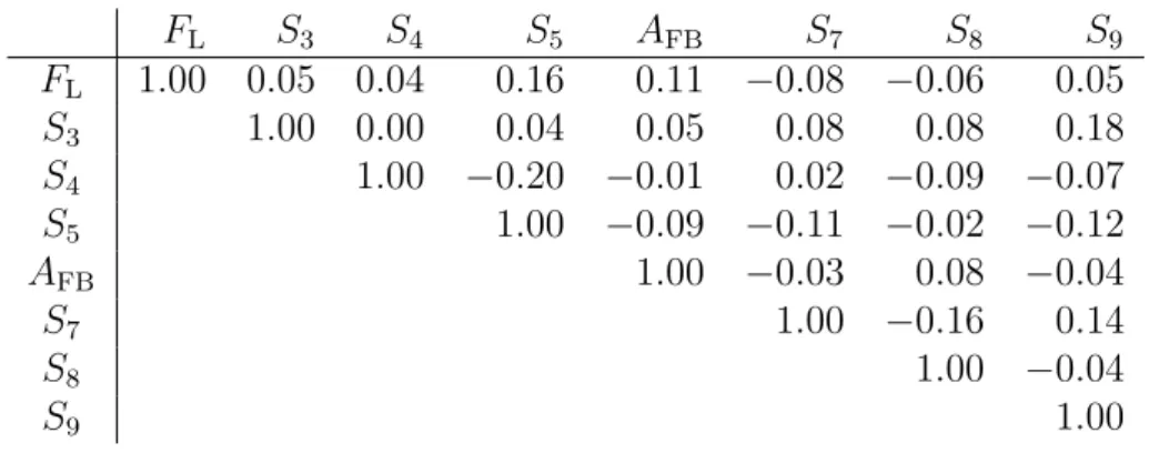
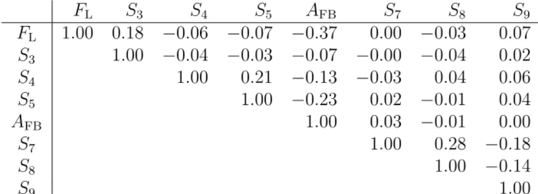
3 Correlation matrices for the CP -averaged

observ-ables

Correlation matrices between the CP -averaged observables in the different q2 bins are provided in Tables 4–13. The different q2 _{bins are statistically independent.}

Table 4: Correlation matrix for the CP -averaged observables from the maximum-likelihood fit in

the bin 0.10 < q2 < 0.98 GeV2/c4.

FL S3 S4 S5 AFB S7 S8 S9 FL 1.00 −0.00 −0.03 0.09 0.03 −0.01 0.06 0.03 S3 1.00 0.02 0.14 0.02 −0.06 0.01 −0.01 S4 1.00 0.06 0.15 −0.03 0.06 0.00 S5 1.00 0.04 −0.03 −0.01 0.00 AFB 1.00 −0.02 −0.01 −0.02 S7 1.00 −0.04 0.10 S8 1.00 0.02 S9 1.00

the bin 1.1 < q2 < 2.5 GeV2/c4.

FL S3 S4 S5 AFB S7 S8 S9 FL 1.00 0.05 0.04 0.16 0.11 −0.08 −0.06 0.05 S3 1.00 0.00 0.04 0.05 0.08 0.08 0.18 S4 1.00 −0.20 −0.01 0.02 −0.09 −0.07 S5 1.00 −0.09 −0.11 −0.02 −0.12 AFB 1.00 −0.03 0.08 −0.04 S7 1.00 −0.16 0.14 S8 1.00 −0.04 S9 1.00

the bin 2.5 < q2 < 4.0 GeV2/c4.

FL S3 S4 S5 AFB S7 S8 S9

FL 1.00 −0.02 −0.03 −0.02 −0.03 −0.01 −0.08 0.06

S3 1.00 −0.05 −0.03 0.05 0.02 −0.07 0.02

(18)

the bin 4.0 < q2 < 6.0 GeV2/c4.

FL S3 S4 S5 AFB S7 S8 S9 FL 1.00 −0.01 0.05 −0.02 −0.14 −0.10 0.09 0.04 S3 1.00 −0.06 −0.10 0.06 −0.02 0.02 −0.08 S4 1.00 0.01 −0.14 0.03 0.02 0.01 S5 1.00 −0.08 0.07 0.02 −0.05 AFB 1.00 −0.01 −0.03 0.01 S7 1.00 0.03 −0.18 S8 1.00 −0.00 S9 1.00

the bin 6.0 < q2 < 8.0 GeV2/c4.

FL S3 S4 S5 AFB S7 S8 S9 FL 1.00 0.00 −0.01 −0.06 −0.20 −0.05 0.00 −0.06 S3 1.00 −0.12 −0.24 0.01 0.05 0.04 −0.10 S4 1.00 0.13 −0.10 0.02 −0.04 −0.04 S5 1.00 −0.16 −0.01 0.02 −0.06 AFB 1.00 −0.03 0.02 0.02 S7 1.00 0.08 −0.09 S8 1.00 −0.08 S9 1.00

the bin 11.0 < q2 < 12.5 GeV2/c4.

FL 1.00 0.14 0.02 −0.09 −0.56 0.02 0.01 0.01

S3 1.00 0.08 −0.08 −0.15 0.02 0.06 −0.10

(19)

Table 10: Correlation matrix for the CP -averaged observables from the maximum-likelihood fit

in the bin 15.0 < q2 < 17.0 GeV2/c4.

FL S3 S4 S5 AFB S7 S8 S9 FL 1.00 0.27 0.02 0.07 −0.53 0.00 −0.04 0.06 S3 1.00 −0.05 0.01 −0.12 −0.02 −0.04 0.10 S4 1.00 0.29 −0.15 0.02 0.06 0.03 S5 1.00 −0.28 0.06 0.03 0.04 AFB 1.00 0.01 −0.00 0.01 S7 1.00 0.31 −0.23 S8 1.00 −0.13 S9 1.00

in the bin 17.0 < q2 < 19.0 GeV2/c4.

FL S3 S4 S5 AFB S7 S8 S9 FL 1.00 0.14 0.06 0.00 −0.35 0.02 −0.02 0.08 S3 1.00 −0.04 −0.15 −0.12 −0.04 0.03 −0.04 S4 1.00 0.25 −0.14 −0.10 0.08 0.02 S5 1.00 −0.25 −0.07 −0.08 0.05 AFB 1.00 −0.00 −0.03 −0.09 S7 1.00 0.33 −0.09 S8 1.00 −0.13 S9 1.00

in the bin 1.1 < q2 < 6.0 GeV2/c4.

FL 1.00 −0.01 −0.02 0.00 0.01 −0.08 0.02 0.03

S3 1.00 −0.04 −0.01 0.04 0.03 0.00 −0.02

(20)

in the bin 15.0 < q2 < 19.0 GeV2/c4.

FL S3 S4 S5 AFB S7 S8 S9 FL 1.00 0.18 −0.06 −0.07 −0.37 0.00 −0.03 0.07 S3 1.00 −0.04 −0.03 −0.07 −0.00 −0.04 0.02 S4 1.00 0.21 −0.13 −0.03 0.04 0.06 S5 1.00 −0.23 0.02 −0.01 0.04 AFB 1.00 0.03 −0.01 0.00 S7 1.00 0.28 −0.18 S8 1.00 −0.14 S9 1.00

(21)

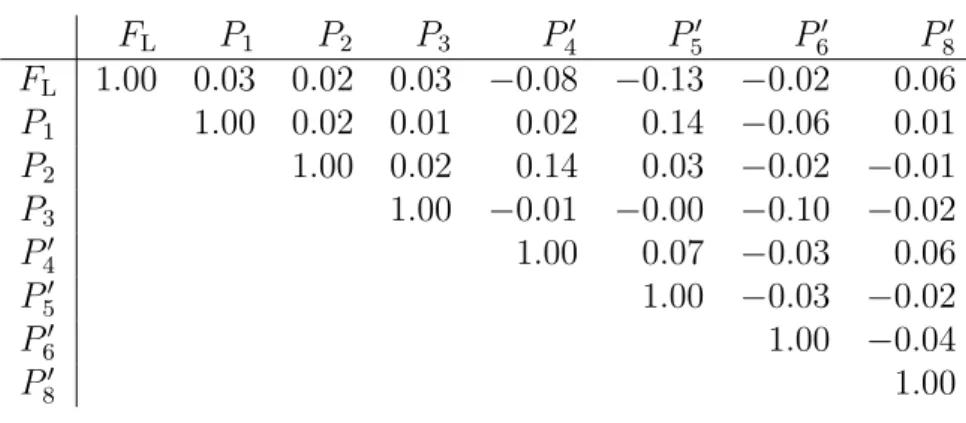
4 Correlation matrices for the optimised angular

ob-servables

Correlation matrices between the optimised P_i(0) basis of observables in the different q2 bins are provided in Tables 14–23.

Table 14: Correlation matrix for the optimised angular observables from the maximum-likelihood

fit in the bin 0.10 < q2 < 0.98 GeV2/c4.

FL P1 P2 P3 P40 P 0 5 P 0 6 P 0 8 FL 1.00 0.03 0.02 0.03 −0.08 −0.13 −0.02 0.06 P1 1.00 0.02 0.01 0.02 0.14 −0.06 0.01 P2 1.00 0.02 0.14 0.03 −0.02 −0.01 P3 1.00 −0.01 −0.00 −0.10 −0.02 P₄0 1.00 0.07 −0.03 0.06 P₅0 1.00 −0.03 −0.02 P₆0 1.00 −0.04 P₈0 1.00

FL P1 P2 P3 P40 P50 P60 P80 FL 1.00 −0.23 −0.51 0.26 0.03 0.24 −0.13 −0.13 P1 1.00 0.15 −0.23 −0.00 −0.02 0.11 0.11 P2 1.00 −0.09 −0.03 −0.22 0.05 0.14 P3 1.00 0.07 0.19 −0.17 −0.00 P₄0 1.00 −0.20 0.02 −0.09 P₅0 1.00 −0.12 −0.04 P₆0 1.00 −0.14 P₈0 1.00

FL P1 P2 P3 P40 P 0 5 P 0 6 P 0 8 FL 1.00 0.08 −0.34 0.01 −0.21 −0.09 −0.08 −0.06 P1 1.00 0.02 −0.02 −0.07 −0.03 0.00 −0.08 P 1.00 0.07 −0.02 −0.05 0.08 −0.03

(22)

FL P1 P2 P3 P40 P 0 5 P 0 6 P 0 8 FL 1.00 0.04 0.05 −0.10 −0.04 −0.14 −0.17 0.14 P1 1.00 0.06 0.07 −0.06 −0.10 −0.03 0.02 P2 1.00 −0.02 −0.14 −0.09 −0.03 −0.01 P3 1.00 −0.01 0.07 0.19 −0.01 P₄0 1.00 0.02 0.04 0.01 P₅0 1.00 0.09 0.00 P₆0 1.00 0.02 P₈0 1.00

FL P1 P2 P3 P40 P 0 5 P 0 6 P 0 8 FL 1.00 −0.02 0.17 0.01 −0.14 −0.18 −0.08 −0.02 P1 1.00 0.01 0.10 −0.12 −0.23 0.04 0.04 P2 1.00 −0.00 −0.13 −0.21 −0.06 0.02 P3 1.00 0.03 0.06 0.09 0.08 P₄0 1.00 0.15 0.03 −0.03 P₅0 1.00 0.00 0.02 P₆0 1.00 0.08 P₈0 1.00

FL P1 P2 P3 P40 P 0 5 P 0 6 P 0 8 FL 1.00 −0.07 0.13 −0.07 0.04 −0.07 0.03 0.00 P1 1.00 −0.09 0.10 0.07 −0.06 0.01 0.05 P2 1.00 −0.16 −0.12 −0.23 −0.05 −0.11

(23)

FL P1 P2 P3 P40 P 0 5 P 0 6 P 0 8 FL 1.00 0.06 0.14 −0.06 0.18 0.23 −0.01 −0.04 P1 1.00 0.03 −0.09 -0.04 0.00 −0.03 −0.04 P2 1.00 −0.06 −0.13 −0.25 0.01 −0.03 P3 1.00 −0.04 −0.05 0.23 0.13 P₄0 1.00 0.32 0.02 0.06 P₅0 1.00 0.06 0.03 P₆0 1.00 0.31 P₈0 1.00

FL P1 P2 P3 P40 P 0 5 P 0 6 P 0 8 FL 1.00 −0.10 0.16 −0.01 0.22 0.14 −0.01 −0.01 P1 1.00 −0.10 0.05 −0.07 −0.16 −0.05 0.03 P2 1.00 0.06 −0.09 −0.23 0.00 −0.05 P3 1.00 −0.01 −0.06 0.09 0.14 P₄0 1.00 0.27 −0.09 0.08 P₅0 1.00 −0.07 −0.09 P₆0 1.00 0.34 P₈0 1.00

FL P1 P2 P3 P40 P 0 5 P 0 6 P 0 8 FL 1.00 −0.05 −0.33 0.09 −0.11 −0.03 −0.14 0.02 P1 1.00 0.05 0.02 −0.04 −0.00 0.03 0.01 P2 1.00 −0.00 −0.04 −0.06 0.03 −0.04

(24)

FL P1 P2 P3 P40 P 0 5 P 0 6 P 0 8 FL 1.00 −0.08 0.19 −0.02 0.11 0.09 −0.01 −0.04 P1 1.00 −0.01 −0.00 −0.04 −0.02 0.00 −0.04 P2 1.00 −0.04 −0.14 −0.25 0.03 −0.03 P3 1.00 −0.06 −0.04 0.18 0.14 P₄0 1.00 0.21 −0.03 0.04 P₅0 1.00 0.02 −0.01 P₆0 1.00 0.28 P₈0 1.00

(25)

5 Fit projections of the signal channel

The angular and mass distributions of the candidates in bins of q2 _{for the Run 1 and the}

2016 data, along with the projections of the simultaneous fit, are shown in Figs. 5–14.

1 − −0.5 0 0.5 1 l θ cos 0 10 20 30 40 Candidates / 0.1 LHCb Run 1 4 c / 2 < 0.98 GeV 2 q 0.10 < 1 − −0.5 0 0.5 1 K θ cos 0 10 20 30 40 Candidates / 0.1 LHCb Run 1 4 c / 2 < 0.98 GeV 2 q 0.10 < 2 − 0 2 φ 0 10 20 30 40 Candidates / 0.31 LHCb Run 1 4 c / 2 < 0.98 GeV 2 q 0.10 < 800 850 900 950 ] 2 c ) [MeV/ − π + K ( m 0 20 40 60 80 2_c Candidates / 10 MeV/ LHCb Run 1 4 c / 2 < 0.98 GeV 2 q 0.10 < 5200 5400 5600 ] 2 c ) [MeV/ − µ + µ − π + K ( m 0 50 100 2_c Candidates / 11 MeV/ LHCb Run 1 4 c / 2 < 0.98 GeV 2 q 0.10 < 1 − −0.5 0 0.5 1 l θ cos 0 10 20 30 40 Candidates / 0.1 LHCb 2016 4 c / 2 < 0.98 GeV 2 q 0.10 < 1 − −0.5 0 0.5 1 K θ cos 0 10 20 30 40 Candidates / 0.1 LHCb 2016 4 c / 2 < 0.98 GeV 2 q 0.10 < 2 − 0 2 φ 0 10 20 30 40 Candidates / 0.31 LHCb 2016 4 c / 2 < 0.98 GeV 2 q 0.10 < 800 850 900 950 ] 2 c ) [MeV/ − π + K ( m 0 20 40 60 80 2 c Candidates / 10 MeV/ LHCb 2016 4 c / 2 < 0.98 GeV 2 q 0.10 < 5200 5400 5600 ] 2 c ) [MeV/ − µ + µ − π + K ( m 0 20 40 60 80 2 c Candidates / 11 MeV/ LHCb 2016 4 c / 2 < 0.98 GeV 2 q 0.10 <

Figure 5: Projections of the fitted probability density function on the decay angles, m(K+π−)

and m(K+π−µ+µ−) for the bin 0.10 < q2 < 0.98 GeV2/c4. The blue shaded region indicates

(26)

1 − −0.5 0 0.5 1 l θ cos 0 10 20 30 Candidates / 0.1 LHCb Run 1 4 c / 2 < 2.5 GeV 2 q 1.1 < 1 − −0.5 0 0.5 1 K θ cos 0 10 20 30 40 Candidates / 0.1 LHCb Run 1 4 c / 2 < 2.5 GeV 2 q 1.1 < 2 − 0 2 φ 0 10 20 30 Candidates / 0.31 LHCb Run 1 4 c / 2 < 2.5 GeV 2 q 1.1 < 800 850 900 950 ] 2 c ) [MeV/ − π + K ( m 0 20 40 2_c Candidates / 10 MeV/ LHCb Run 1 4 c / 2 < 2.5 GeV 2 q 1.1 < 5200 5400 5600 ] 2 c ) [MeV/ − µ + µ − π + K ( m 0 20 40 60 80 2_c Candidates / 11 MeV/ LHCb Run 1 4 c / 2 < 2.5 GeV 2 q 1.1 < 1 − −0.5 0 0.5 1 l θ cos 0 10 20 30 40 Candidates / 0.1 LHCb 2016 4 c / 2 < 2.5 GeV 2 q 1.1 < 1 − −0.5 0 0.5 1 K θ cos 0 20 40 Candidates / 0.1 LHCb 2016 4 c / 2 < 2.5 GeV 2 q 1.1 < 2 − 0 2 φ 0 10 20 30 Candidates / 0.31 LHCb 2016 4 c / 2 < 2.5 GeV 2 q 1.1 < 800 850 900 950 ] 2 c ) [MeV/ − π + K ( m 0 20 40 2 c Candidates / 10 MeV/ LHCb 2016 4 c / 2 < 2.5 GeV 2 q 1.1 < 5200 5400 5600 ] 2 c ) [MeV/ − µ + µ − π + K ( m 0 20 40 60 2 c Candidates / 11 MeV/ LHCb 2016 4 c / 2 < 2.5 GeV 2 q 1.1 <

Figure 6: Projections of the fitted probability density function on the decay angles, m(K+_π−₎

(27)

1 − −0.5 0 0.5 1 l θ cos 0 10 20 30 40 Candidates / 0.1 LHCb Run 1 4 c / 2 < 4.0 GeV 2 q 2.5 < 1 − −0.5 0 0.5 1 K θ cos 0 20 40 Candidates / 0.1 LHCb Run 1 4 c / 2 < 4.0 GeV 2 q 2.5 < 2 − 0 2 φ 0 10 20 30 40 Candidates / 0.31 LHCb Run 1 4 c / 2 < 4.0 GeV 2 q 2.5 < 800 850 900 950 ] 2 c ) [MeV/ − π + K ( m 0 20 40 60 2_c Candidates / 10 MeV/ LHCb Run 1 4 c / 2 < 4.0 GeV 2 q 2.5 < 5200 5400 5600 ] 2 c ) [MeV/ − µ + µ − π + K ( m 0 20 40 60 2_c Candidates / 11 MeV/ LHCb Run 1 4 c / 2 < 4.0 GeV 2 q 2.5 < 1 − −0.5 0 0.5 1 l θ cos 0 10 20 30 40 Candidates / 0.1 LHCb 2016 4 c / 2 < 4.0 GeV 2 q 2.5 < 1 − −0.5 0 0.5 1 K θ cos 0 20 40 Candidates / 0.1 LHCb 2016 4 c / 2 < 4.0 GeV 2 q 2.5 < 2 − 0 2 φ 0 10 20 30 Candidates / 0.31 LHCb 2016 4 c / 2 < 4.0 GeV 2 q 2.5 < 800 850 900 950 ] 2 c ) [MeV/ − π + K ( m 0 20 40 2 c Candidates / 10 MeV/ LHCb 2016 4 c / 2 < 4.0 GeV 2 q 2.5 < 5200 5400 5600 ] 2 c ) [MeV/ − µ + µ − π + K ( m 0 20 40 2 c Candidates / 11 MeV/ LHCb 2016 4 c / 2 < 4.0 GeV 2 q 2.5 <

(28)

1 − −0.5 0 0.5 1 l θ cos 0 20 40 60 Candidates / 0.1 LHCb Run 1 4 c / 2 < 6.0 GeV 2 q 4.0 < 1 − −0.5 0 0.5 1 K θ cos 0 20 40 60 80 Candidates / 0.1 LHCb Run 1 4 c / 2 < 6.0 GeV 2 q 4.0 < 2 − 0 2 φ 0 20 40 Candidates / 0.31 LHCb Run 1 4 c / 2 < 6.0 GeV 2 q 4.0 < 800 850 900 950 ] 2 c ) [MeV/ − π + K ( m 0 50 100 2_c Candidates / 10 MeV/ LHCb Run 1 4 c / 2 < 6.0 GeV 2 q 4.0 < 5200 5400 5600 ] 2 c ) [MeV/ − µ + µ − π + K ( m 0 50 100 2_c Candidates / 11 MeV/ LHCb Run 1 4 c / 2 < 6.0 GeV 2 q 4.0 < 1 − −0.5 0 0.5 1 l θ cos 0 10 20 30 40 Candidates / 0.1 LHCb 2016 4 c / 2 < 6.0 GeV 2 q 4.0 < 1 − −0.5 0 0.5 1 K θ cos 0 20 40 60 Candidates / 0.1 LHCb 2016 4 c / 2 < 6.0 GeV 2 q 4.0 < 2 − 0 2 φ 0 10 20 30 40 Candidates / 0.31 LHCb 2016 4 c / 2 < 6.0 GeV 2 q 4.0 < 800 850 900 950 ] 2 c ) [MeV/ − π + K ( m 0 20 40 60 80 2 c Candidates / 10 MeV/ LHCb 2016 4 c / 2 < 6.0 GeV 2 q 4.0 < 5200 5400 5600 ] 2 c ) [MeV/ − µ + µ − π + K ( m 0 20 40 60 80 2 c Candidates / 11 MeV/ LHCb 2016 4 c / 2 < 6.0 GeV 2 q 4.0 <

(29)

1 − −0.5 0 0.5 1 l θ cos 0 20 40 60 80 Candidates / 0.1 LHCb Run 1 4 c / 2 < 8.0 GeV 2 q 6.0 < 1 − −0.5 0 0.5 1 K θ cos 0 20 40 60 80 Candidates / 0.1 LHCb Run 1 4 c / 2 < 8.0 GeV 2 q 6.0 < 2 − 0 2 φ 0 20 40 60 Candidates / 0.31 LHCb Run 1 4 c / 2 < 8.0 GeV 2 q 6.0 < 800 850 900 950 ] 2 c ) [MeV/ − π + K ( m 0 50 100 2_c Candidates / 10 MeV/ LHCb Run 1 4 c / 2 < 8.0 GeV 2 q 6.0 < 5200 5400 5600 ] 2 c ) [MeV/ − µ + µ − π + K ( m 0 50 100 150 2_c Candidates / 11 MeV/ LHCb Run 1 4 c / 2 < 8.0 GeV 2 q 6.0 < 1 − −0.5 0 0.5 1 l θ cos 0 20 40 60 Candidates / 0.1 LHCb 2016 4 c / 2 < 8.0 GeV 2 q 6.0 < 1 − −0.5 0 0.5 1 K θ cos 0 20 40 60 80 Candidates / 0.1 LHCb 2016 4 c / 2 < 8.0 GeV 2 q 6.0 < 2 − 0 2 φ 0 20 40 60 Candidates / 0.31 LHCb 2016 4 c / 2 < 8.0 GeV 2 q 6.0 < 800 850 900 950 ] 2 c ) [MeV/ − π + K ( m 0 50 100 2 c Candidates / 10 MeV/ LHCb 2016 4 c / 2 < 8.0 GeV 2 q 6.0 < 5200 5400 5600 ] 2 c ) [MeV/ − µ + µ − π + K ( m 0 50 100 2 c Candidates / 11 MeV/ LHCb 2016 4 c / 2 < 8.0 GeV 2 q 6.0 <

(30)

1 − −0.5 0 0.5 1 l θ cos 0 20 40 60 Candidates / 0.1 LHCb Run 1 4 c / 2 < 12.5 GeV 2 q 11.0 < 1 − −0.5 0 0.5 1 K θ cos 0 20 40 60 Candidates / 0.1 LHCb Run 1 4 c / 2 < 12.5 GeV 2 q 11.0 < 2 − 0 2 φ 0 20 40 Candidates / 0.31 LHCb Run 1 4 c / 2 < 12.5 GeV 2 q 11.0 < 800 850 900 950 ] 2 c ) [MeV/ − π + K ( m 0 50 100 2_c Candidates / 10 MeV/ LHCb Run 1 4 c / 2 < 12.5 GeV 2 q 11.0 < 5200 5400 5600 ] 2 c ) [MeV/ − µ + µ − π + K ( m 0 50 100 2_c Candidates / 11 MeV/ LHCb Run 1 4 c / 2 < 12.5 GeV 2 q 11.0 < 1 − −0.5 0 0.5 1 l θ cos 0 20 40 60 Candidates / 0.1 LHCb 2016 4 c / 2 < 12.5 GeV 2 q 11.0 < 1 − −0.5 0 0.5 1 K θ cos 0 10 20 30 40 Candidates / 0.1 LHCb 2016 4 c / 2 < 12.5 GeV 2 q 11.0 < 2 − 0 2 φ 0 10 20 30 40 Candidates / 0.31 LHCb 2016 4 c / 2 < 12.5 GeV 2 q 11.0 < 800 850 900 950 ] 2 c ) [MeV/ − π + K ( m 0 20 40 60 80 2 c Candidates / 10 MeV/ LHCb 2016 4 c / 2 < 12.5 GeV 2 q 11.0 < 5200 5400 5600 ] 2 c ) [MeV/ − µ + µ − π + K ( m 0 20 40 60 80 2 c Candidates / 11 MeV/ LHCb 2016 4 c / 2 < 12.5 GeV 2 q 11.0 <

(31)

1 − −0.5 0 0.5 1 l θ cos 0 20 40 60 80 Candidates / 0.1 LHCb Run 1 4 c / 2 < 17.0 GeV 2 q 15.0 < 1 − −0.5 0 0.5 1 K θ cos 0 20 40 60 Candidates / 0.1 LHCb Run 1 4 c / 2 < 17.0 GeV 2 q 15.0 < 2 − 0 2 φ 0 20 40 60 Candidates / 0.31 LHCb Run 1 4 c / 2 < 17.0 GeV 2 q 15.0 < 800 850 900 950 ] 2 c ) [MeV/ − π + K ( m 0 50 100 2_c Candidates / 10 MeV/ LHCb Run 1 4 c / 2 < 17.0 GeV 2 q 15.0 < 5200 5400 5600 ] 2 c ) [MeV/ − µ + µ − π + K ( m 0 50 100 150 2_c Candidates / 11 MeV/ LHCb Run 1 4 c / 2 < 17.0 GeV 2 q 15.0 < 1 − −0.5 0 0.5 1 l θ cos 0 20 40 60 80 Candidates / 0.1 LHCb 2016 4 c / 2 < 17.0 GeV 2 q 15.0 < 1 − −0.5 0 0.5 1 K θ cos 0 20 40 60 Candidates / 0.1 LHCb 2016 4 c / 2 < 17.0 GeV 2 q 15.0 < 2 − 0 2 φ 0 20 40 Candidates / 0.31 LHCb 2016 4 c / 2 < 17.0 GeV 2 q 15.0 < 800 850 900 950 ] 2 c ) [MeV/ − π + K ( m 0 50 100 2 c Candidates / 10 MeV/ LHCb 2016 4 c / 2 < 17.0 GeV 2 q 15.0 < 5200 5400 5600 ] 2 c ) [MeV/ − µ + µ − π + K ( m 0 50 100 2 c Candidates / 11 MeV/ LHCb 2016 4 c / 2 < 17.0 GeV 2 q 15.0 <

(32)

1 − −0.5 0 0.5 1 l θ cos 0 20 40 60 Candidates / 0.1 LHCb Run 1 4 c / 2 < 19.0 GeV 2 q 17.0 < 1 − −0.5 0 0.5 1 K θ cos 0 20 40 Candidates / 0.1 LHCb Run 1 4 c / 2 < 19.0 GeV 2 q 17.0 < 2 − 0 2 φ 0 10 20 30 40 Candidates / 0.31 LHCb Run 1 4 c / 2 < 19.0 GeV 2 q 17.0 < 800 850 900 950 ] 2 c ) [MeV/ − π + K ( m 0 20 40 60 80 2_c Candidates / 10 MeV/ LHCb Run 1 4 c / 2 < 19.0 GeV 2 q 17.0 < 5200 5400 5600 ] 2 c ) [MeV/ − µ + µ − π + K ( m 0 50 100 2_c Candidates / 11 MeV/ LHCb Run 1 4 c / 2 < 19.0 GeV 2 q 17.0 < 1 − −0.5 0 0.5 1 l θ cos 0 20 40 60 Candidates / 0.1 LHCb 2016 4 c / 2 < 19.0 GeV 2 q 17.0 < 1 − −0.5 0 0.5 1 K θ cos 0 10 20 30 Candidates / 0.1 LHCb 2016 4 c / 2 < 19.0 GeV 2 q 17.0 < 2 − 0 2 φ 0 10 20 30 Candidates / 0.31 LHCb 2016 4 c / 2 < 19.0 GeV 2 q 17.0 < 800 850 900 950 ] 2 c ) [MeV/ − π + K ( m 0 20 40 60 80 2 c Candidates / 10 MeV/ LHCb 2016 4 c / 2 < 19.0 GeV 2 q 17.0 < 5200 5400 5600 ] 2 c ) [MeV/ − µ + µ − π + K ( m 0 20 40 60 2 c Candidates / 11 MeV/ LHCb 2016 4 c / 2 < 19.0 GeV 2 q 17.0 <

(33)

1 − −0.5 0 0.5 1 l θ cos 0 50 100 150 Candidates / 0.1 LHCb Run 1 4 c / 2 < 6.0 GeV 2 q 1.1 < 1 − −0.5 0 0.5 1 K θ cos 0 100 200 Candidates / 0.1 LHCb Run 1 4 c / 2 < 6.0 GeV 2 q 1.1 < 2 − 0 2 φ 0 50 100 150 Candidates / 0.31 LHCb Run 1 4 c / 2 < 6.0 GeV 2 q 1.1 < 800 850 900 950 ] 2 c ) [MeV/ − π + K ( m 0 100 200 2_c Candidates / 10 MeV/ LHCb Run 1 4 c / 2 < 6.0 GeV 2 q 1.1 < 5200 5400 5600 ] 2 c ) [MeV/ − µ + µ − π + K ( m 0 100 200 300 2_c Candidates / 11 MeV/ LHCb Run 1 4 c / 2 < 6.0 GeV 2 q 1.1 < 1 − −0.5 0 0.5 1 l θ cos 0 50 100 Candidates / 0.1 LHCb 2016 4 c / 2 < 6.0 GeV 2 q 1.1 < 1 − −0.5 0 0.5 1 K θ cos 0 50 100 150 Candidates / 0.1 LHCb 2016 4 c / 2 < 6.0 GeV 2 q 1.1 < 2 − 0 2 φ 0 50 100 Candidates / 0.31 LHCb 2016 4 c / 2 < 6.0 GeV 2 q 1.1 < 800 850 900 950 ] 2 c ) [MeV/ − π + K ( m 0 50 100 150 200 2 c Candidates / 10 MeV/ LHCb 2016 4 c / 2 < 6.0 GeV 2 q 1.1 < 5200 5400 5600 ] 2 c ) [MeV/ − µ + µ − π + K ( m 0 100 200 2 c Candidates / 11 MeV/ LHCb 2016 4 c / 2 < 6.0 GeV 2 q 1.1 <

(34)

1 − −0.5 0 0.5 1 l θ cos 0 50 100 150 Candidates / 0.1 LHCb Run 1 4 c / 2 < 19.0 GeV 2 q 15.0 < 1 − −0.5 0 0.5 1 K θ cos 0 50 100 Candidates / 0.1 LHCb Run 1 4 c / 2 < 19.0 GeV 2 q 15.0 < 2 − 0 2 φ 0 50 100 Candidates / 0.31 LHCb Run 1 4 c / 2 < 19.0 GeV 2 q 15.0 < 800 850 900 950 ] 2 c ) [MeV/ − π + K ( m 0 50 100 150 200 2_c Candidates / 10 MeV/ LHCb Run 1 4 c / 2 < 19.0 GeV 2 q 15.0 < 5200 5400 5600 ] 2 c ) [MeV/ − µ + µ − π + K ( m 0 100 200 2_c Candidates / 11 MeV/ LHCb Run 1 4 c / 2 < 19.0 GeV 2 q 15.0 < 1 − −0.5 0 0.5 1 l θ cos 0 50 100 Candidates / 0.1 LHCb 2016 4 c / 2 < 19.0 GeV 2 q 15.0 < 1 − −0.5 0 0.5 1 K θ cos 0 50 100 Candidates / 0.1 LHCb 2016 4 c / 2 < 19.0 GeV 2 q 15.0 < 2 − 0 2 φ 0 50 100 Candidates / 0.31 LHCb 2016 4 c / 2 < 19.0 GeV 2 q 15.0 < 800 850 900 950 ] 2 c ) [MeV/ − π + K ( m 0 50 100 150 200 2 c Candidates / 10 MeV/ LHCb 2016 4 c / 2 < 19.0 GeV 2 q 15.0 < 5200 5400 5600 ] 2 c ) [MeV/ − µ + µ − π + K ( m 0 50 100 150 200 2 c Candidates / 11 MeV/ LHCb 2016 4 c / 2 < 19.0 GeV 2 q 15.0 <

(35)

References

[1] LHCb collaboration, R. Aaij et al., Angular analysis of the B0_{→ K}∗0_µ+_µ− _decay

using 3 fb−1 of integrated luminosity, JHEP 02 (2016) 104, arXiv:1512.04442. [2] CMS collaboration, A. M. Sirunyan et al., Measurement of angular parameters from

the decay B0_{→ K}∗0_µ+_µ− _{in proton-proton collisions at} √_{s = 8 TeV, Phys. Lett.}

B781 (2018) 517, arXiv:1710.02846.

[3] ATLAS collaboration, M. Aaboud et al., Angular analysis of B0

d → K

∗_µ+_µ− _decays

in pp collisions at √s = 8 TeV with the ATLAS detector, JHEP 10 (2018) 047, arXiv:1805.04000.

[4] Belle collaboration, S. Wehle et al., Lepton-flavor-dependent angular analysis of B → K∗`+`−, Phys. Rev. Lett. 118 (2017) 111801, arXiv:1612.05014.

[5] BaBar collaboration, B. Aubert et al., Measurements of branching fractions, rate asym-metries, and angular distributions in the rare decays B → K`+_`− _{and B → K}∗_`+_`−_,

Phys. Rev. D73 (2006) 092001, arXiv:hep-ex/0604007.

[6] CDF collaboration, T. Aaltonen et al., Measurements of the angular distribu-tions in the decays B → K(∗)_µ+_µ− _{at CDF, Phys. Rev. Lett. 108 (2012) 081807,}

arXiv:1108.0695.

[7] LHCb collaboration, R. Aaij et al., Angular moments of the decay Λ0

b→ Λµ+µ

− _at

low hadronic recoil, JHEP 09 (2018) 146, arXiv:1808.00264.

[8] LHCb collaboration, R. Aaij et al., Angular analysis and differential branching fraction of the decay B0

s→ φµ+µ

−_{, JHEP 09 (2015) 179, arXiv:1506.08777.}

[9] LHCb collaboration, R. Aaij et al., Measurements of the S-wave fraction in B0→ K+_π−

µ+µ− decays and the B0→ K∗(892)0µ+µ− differential branching fraction, JHEP 11 (2016) 047, Erratum ibid. 04 (2017) 142, arXiv:1606.04731.

[10] LHCb collaboration, R. Aaij et al., Differential branching fraction and angular analysis of Λ0

b→ Λµ+µ

− _{decays, JHEP 06 (2015) 115, Erratum ibid. 09 (2018) 145,}

arXiv:1503.07138.

[11] LHCb collaboration, R. Aaij et al., Differential branching fractions and isospin asymmetries of B → K(∗)_µ+_µ− _{decays, JHEP 06 (2014) 133, arXiv:1403.8044.}

[12] LHCb collaboration, R. Aaij et al., Search for lepton-universality violation in B+→ K+_`+_`− _{decays, Phys. Rev. Lett. 122 (2019) 191801, arXiv:1903.09252.}

(36)

[15] LHCb collaboration, R. Aaij et al., Test of lepton universality with B0_{→ K}∗0_`+_`−

decays, JHEP 08 (2017) 055, arXiv:1705.05802.

[16] Belle collaboration, A. Abdesselam et al., Test of lepton flavor universality in B → K∗`+_`− _{decays at Belle, arXiv:1904.02440.}

[17] M. Alguer´o et al., Emerging patterns of new physics with and without Lepton flavour universal contributions, Eur. Phys. J. C79 (2019) 714, arXiv:1903.09578.

[18] J. Aebischer et al., B-decay discrepancies after Moriond 2019, arXiv:1903.10434. [19] A. Arbey et al., Update on the b → s anomalies, Phys. Rev. D100 (2019) 015045,

arXiv:1904.08399.

[20] M. Ciuchini et al., New physics in b → s`+`− confronts new data on lepton universality, Eur. Phys. J. C79 (2019) 719, arXiv:1903.09632.

[21] K. Kowalska, D. Kumar, and E. M. Sessolo, Implications for new physics in b → sµµ transitions after recent measurements by Belle and LHCb, Eur. Phys. J. C79 (2019) 840, arXiv:1903.10932.

[22] A. K. Alok, A. Dighe, S. Gangal, and D. Kumar, Continuing search for new physics in b → sµµ decays: Two operators at a time, JHEP 06 (2019) 089, arXiv:1903.09617. [23] W. Altmannshofer, S. Gori, M. Pospelov, and I. Yavin, Quark flavor transitions in

Lµ− Lτ models, Phys. Rev. D89 (2014) 095033, arXiv:1403.1269.

[24] A. Crivellin, G. D’Ambrosio, and J. Heeck, Explaining h → µ±τ∓, B → K∗µ+_µ−

and B → Kµ+_µ−_{/B → Ke}+_e− _{in a two-Higgs-doublet model with gauged L}

µ− Lτ,

Phys. Rev. Lett. 114 (2015) 151801, arXiv:1501.00993.

[25] A. Celis, J. Fuentes-Mart´ın, M. Jung, and H. Serˆodio, Family nonuniversal Z0 models with protected flavor-changing interactions, Phys. Rev. D92 (2015) 015007, arXiv:1505.03079.

[26] A. Falkowski, M. Nardecchia, and R. Ziegler, Lepton flavor non-universality in B-meson decays from a U (2) flavor model, JHEP 11 (2015) 173, arXiv:1509.01249. [27] G. Hiller and M. Schmaltz, RK and future b → s`` physics beyond the standard model

opportunities, Phys. Rev. D90 (2014) 054014, arXiv:1408.1627.

[28] B. Gripaios, M. Nardecchia, and S. A. Renner, Composite leptoquarks and anomalies in B-meson decays, JHEP 05 (2015) 006, arXiv:1412.1791.

[29] I. de Medeiros Varzielas and G. Hiller, Clues for flavor from rare lepton and quark decays, JHEP 06 (2015) 072, arXiv:1503.01084.

(37)

[32] G. Hiller, D. Loose, and I. Ni˘sand˘zi´c, Flavorful leptoquarks at hadron colliders, Phys. Rev. D97 (2018) 075004, arXiv:1801.09399.

[33] A. Crivellin, D. M¨uller, and T. Ota, Simultaneous explanation of R(D(∗)) and b → sµ+_µ−_: _{the last scalar leptoquarks standing, JHEP 09 (2017) 040,}

arXiv:1703.09226.

[34] F. Sala and D. M. Straub, A new light particle in B decays?, Phys. Lett. B774 (2017) 205209.

[35] P. Ko, Y. Omura, Y. Shigekami, and C. Yu, LHCb anomaly and B physics in flavored Z0 models with flavored Higgs doublets, Phys. Rev. D95 (2017) 115040.

[36] S. J¨ager and J. Martin Camalich, Reassessing the discovery potential of the B → K∗`+_`− _{decays in the large-recoil region: SM challenges and BSM}

opportu-nities, Phys. Rev. D93 (2016) 014028, arXiv:1412.3183.

[37] J. Lyon and R. Zwicky, Resonances gone topsy turvy - the charm of QCD or new physics in b → s`+_`−_{?, arXiv:1406.0566.}

[38] M. Ciuchini et al., B → K∗`+`− decays at large recoil in the Standard Model: a theoretical reappraisal, JHEP 06 (2016) 116, arXiv:1512.07157.

[39] C. Bobeth, M. Chrzaszcz, D. van Dyk, and J. Virto, Long-distance effects in B → K∗`` from analyticity, Eur. Phys. J. C78 (2018) 451, arXiv:1707.07305.

[40] F. Beaujean, C. Bobeth, and D. van Dyk, Comprehensive Bayesian analysis of rare (semi)leptonic and radiative B decays, Eur. Phys. J. C74 (2014) 2897, arXiv:1310.2478.

[41] C. Bobeth, G. Hiller, and D. van Dyk, The benefits of B → K∗l+_l− _{decays at low}

recoil, JHEP 07 (2010) 098, arXiv:1006.5013.

[42] D. M. Straub, flavio: A python package for flavour and precision phenomenology in the Standard Model and beyond, arXiv:1810.08132.

[43] A. Bharucha, D. M. Straub, and R. Zwicky, B → V `+`− in the Standard Model from light-cone sum rules, JHEP 08 (2016) 098, arXiv:1503.05534.

[44] W. Altmannshofer and D. M. Straub, New physics in b → s transitions after LHC run 1, Eur. Phys. J. C75 (2015) 382, arXiv:1411.3161.

[45] LHCb collaboration, R. Aaij et al., Measurement of the B± production cross-section in pp collisions at √s =7 and 13 TeV, JHEP 12 (2017) 026, arXiv:1710.04921.

(38)

[48] S. Descotes-Genon, J. Matias, M. Ramon, and J. Virto, Implications from clean observables for the binned analysis of B → K∗µ+_µ− _{at large recoil, JHEP 01 (2013)}

048, arXiv:1207.2753.

[49] LHCb collaboration, A. A. Alves Jr. et al., The LHCb detector at the LHC, JINST 3 (2008) S08005.

[50] LHCb collaboration, R. Aaij et al., LHCb detector performance, Int. J. Mod. Phys. A30 (2015) 1530022, arXiv:1412.6352.

[51] T. Sj¨ostrand, S. Mrenna, and P. Skands, PYTHIA 6.4 physics and manual, JHEP 05 (2006) 026, arXiv:hep-ph/0603175; T. Sj¨ostrand, S. Mrenna, and P. Skands, A brief introduction to PYTHIA 8.1, Comput. Phys. Commun. 178 (2008) 852, arXiv:0710.3820.

[52] I. Belyaev et al., Handling of the generation of primary events in Gauss, the LHCb simulation framework, J. Phys. Conf. Ser. 331 (2011) 032047.

[53] D. J. Lange, The EvtGen particle decay simulation package, Nucl. Instrum. Meth. A462 (2001) 152.

[54] P. Golonka and Z. Was, PHOTOS Monte Carlo: A precision tool for QED corrections in Z and W decays, Eur. Phys. J. C45 (2006) 97, arXiv:hep-ph/0506026.

[55] Geant4 collaboration, J. Allison et al., Geant4 developments and applications, IEEE Trans. Nucl. Sci. 53 (2006) 270; Geant4 collaboration, S. Agostinelli et al., Geant4: A simulation toolkit, Nucl. Instrum. Meth. A506 (2003) 250.

[56] M. Clemencic et al., The LHCb simulation application, Gauss: Design, evolution and experience, J. Phys. Conf. Ser. 331 (2011) 032023.

[57] L. Anderlini et al., The PIDCalib package, LHCb-PUB-2016-021, CERN, Geneva, 2016.

[58] R. Aaij et al., Selection and processing of calibration samples to measure the particle identification performance of the LHCb experiment in Run 2, EPJ Tech. Instrum. 6 (2019) 1, arXiv:1803.00824.

[59] R. Aaij et al., The LHCb trigger and its performance in 2011, JINST 8 (2013) P04022, arXiv:1211.3055.

[60] L. Breiman, J. H. Friedman, R. A. Olshen, and C. J. Stone, Classification and regression trees, Wadsworth international group, Belmont, California, USA, 1984. [61] Y. Freund and R. E. Schapire, A decision-theoretic generalization of on-line learning

(39)

[63] LHCb collaboration, R. Aaij et al., Search for the rare decays B0

s→ µ+µ

− _and

B0_{→ µ}+_µ−_{, Phys. Lett. B699 (2011) 330, arXiv:1103.2465.}

[64] B. Efron, Bootstrap methods: Another look at the jackknife, Ann. Statist. 7 (1979) 1. [65] LHCb collaboration, R. Aaij et al., Evidence for the decay B0

s→ K

∗0_µ+_µ−_{, JHEP 07}

(2018) 020, arXiv:1804.07167.

[66] D. Aston et al., A Study of K−π+ scattering in the reaction K−π+ → K−_π+_{n at}

11 GeV/c, Nucl. Phys. B296 (1988) 493.

[67] BaBar collaboration, B. Aubert et al., Measurement of decay amplitudes of B → J/ψK∗, ψ(2S)K∗, and χc1K∗ with an angular analysis, Phys. Rev. D76 (2007)

031102, arXiv:0704.0522.

[68] Belle collaboration, K. Chilikin et al., Observation of a new charged charmonium like state in ¯B0 → J/ψK−_π+ _{decays, Phys. Rev. D90 (2014) 112009, arXiv:1408.6457.}

[69] LHCb collaboration, R. Aaij et al., Measurement of the polarization amplitudes in B0 → J/ψK∗₍₈₉₂₎0 _{decays, Phys. Rev. D88 (2013) 052002, arXiv:1307.2782.}

[70] S. Descotes-Genon, L. Hofer, J. Matias, and J. Virto, On the impact of power corrections in the prediction of B → K∗µ+_µ− _{observables, JHEP 12 (2014) 125,}

arXiv:1407.8526.

[71] A. Khodjamirian, T. Mannel, A. A. Pivovarov, and Y.-M. Wang, Charm-loop effect in B → K(∗)_`+_`− _{and B → K}∗_{γ, JHEP 09 (2010) 089, arXiv:1006.4945.}

[72] R. R. Horgan, Z. Liu, S. Meinel, and M. Wingate, Lattice QCD calculation of form factors describing the rare decays B → K∗`+_`− _{and B}

s→ φ`+`−, Phys. Rev. D89

(2014) 094501, arXiv:1310.3722.

[73] R. R. Horgan, Z. Liu, S. Meinel, and M. Wingate, Rare B decays using lattice QCD form factors, PoS LATTICE2014 (2015) 372, arXiv:1501.00367.