HAL Id: hal-02939160
https://hal.inrae.fr/hal-02939160
Submitted on 15 Sep 2020HAL is a multi-disciplinary open access archive for the deposit and dissemination of sci-entific research documents, whether they are pub-lished or not. The documents may come from teaching and research institutions in France or abroad, or from public or private research centers.
L’archive ouverte pluridisciplinaire HAL, est destinée au dépôt et à la diffusion de documents scientifiques de niveau recherche, publiés ou non, émanant des établissements d’enseignement et de recherche français ou étrangers, des laboratoires publics ou privés.
Estimating leaf mass per area and equivalent water
thickness based on leaf optical properties: potential and
limitations of physical modeling and machine learning.
Jean-Baptiste Féret, G. Le Maire, S. Jay, D. Berveiller, Ryad Bendoula, G.
Hmimina, A. Cheraiet, J.C. Oliveira, F.J. Ponzoni, T. Solanki, et al.
To cite this version:
Jean-Baptiste Féret, G. Le Maire, S. Jay, D. Berveiller, Ryad Bendoula, et al.. Estimating leaf mass per area and equivalent water thickness based on leaf optical properties: potential and limitations of physical modeling and machine learning.. Remote Sensing of Environment, Elsevier, 2019, 231, �10.1016/j.rse.2018.11.002�. �hal-02939160�
1
Estimating leaf mass per area and equivalent water thickness based on leaf optical properties: 1
potential and limitations of physical modeling and machine learning. 2
J.-B. Féret1, G. le Maire2,3,4, S. Jay5, D. Berveiller6, R. Bendoula7, G. Hmimina6, A. Cheraiet6, J.C. 3
Oliveira8, F.J. Ponzoni9, T. Solanki10, F. de Boissieu1, J. Chave11, Y. Nouvellon2,3,12, A. Porcar-Castell10, C. 4
Proisy13,14, K. Soudani6, J.-P. Gastellu-Etchegorry15, M.-J. Lefèvre-Fonollosa16 5
1
TETIS, Irstea, AgroParisTech, CIRAD, CNRS, Université Montpellier, Montpellier, France 6
2
CIRAD, UMR ECO&SOLS, Montpellier, France 7
3
Eco&Sols, Univ Montpellier, CIRAD, INRA, IRD, Montpellier SupAgro, Montpellier, France. 8
4
Interdisciplinary Center of Energy Planning (NIPE), UNICAMP, 13083-896 Campinas, Brazil 9
5
Aix Marseille Univ, CNRS, Centrale Marseille, Institut Fresnel, F-13013 Marseille, France 10
6
Ecologie Systematique Evolution, University of Paris-Sud, CNRS, AgroParisTech, Université Paris 11
Saclay, F-91400 Orsay, France 12
7
ITAP, Irstea, Montpellier SupAgro, Université Montpellier, Montpellier, France 13
8
School of Agricultural Engineering - FEAGRI, University of Campinas, São Paulo, Brazil 14
9
Instituto Nacional de Pesquisas Espaciais, Sao Jose dos Campos 12227-010, Brazil 15
10
Optics of Photosynthesis Laboratory, INAR/Forests, Faculty of Agriculture and Forestry, 00014 16
University of Helsinki, Finland 17
11
Laboratoire Evolution et Diversité Biologique UMR 5174, CNRS, Université Paul Sabatier, Toulouse, 18
France 19
12
University of Sao Paulo, ESALQ/USP, Piracicaba 13418-900, Brazil 20
13
AMAP, IRD, CIRAD, CNRS, INRA, Univ. Montpellier, Montpellier, France 21
14
GEOSMIT, French Institute of Pondicherry, Pondicherry, India 22
15
Centre d’Etudes Spatiales de la Biosphère, Toulouse 31400, France 23
16
CNES 24
2
Abstract
25
Leaf mass per area (𝐿𝑀𝐴) and leaf equivalent water thickness (𝐸𝑊𝑇) are key leaf functional traits 26
providing information for many applications including ecosystem functioning modeling and fire risk 27
management. In this paper, we investigate two common conclusions generally made for 𝐿𝑀𝐴 and 28
𝐸𝑊𝑇 estimation based on leaf optical properties in the near-infrared (NIR) and shortwave infrared 29
(SWIR) domains: (1) physically-based approaches estimate 𝐸𝑊𝑇 accurately and 𝐿𝑀𝐴 poorly, while 30
(2) statistically-based and machine learning (ML) methods provide accurate estimates of both 𝐿𝑀𝐴 31
and 𝐸𝑊𝑇. 32
Using six experimental datasets including broadleaf species samples of more than 150 species 33
collected over tropical, temperate and boreal ecosystems, we compared the performances of a 34
physically-based method (PROSPECT model inversion) and a ML algorithm (support vector machine 35
regressions, SVM) to infer 𝐸𝑊𝑇 and 𝐿𝑀𝐴 based on leaf reflectance and transmittance. We assessed 36
several merit functions to invert PROSPECT based on iterative optimization and investigated the 37
spectral domain to be used for optimal estimation of 𝐿𝑀𝐴 and 𝐸𝑊𝑇. We also tested several 38
strategies to select the training samples used by the SVM, in order to investigate the generalization 39
ability of the derived regression models. 40
We evidenced that using spectral information from 1700 to 2400 nm leads to strong improvement in 41
the estimation of 𝐸𝑊𝑇 and 𝐿𝑀𝐴 when performing a PROSPECT inversion, decreasing the 𝐿𝑀𝐴 and 42
𝐸𝑊𝑇 estimation errors by 55% and 33%, respectively. 43
The comparison of various sampling strategies for the training set used with SVM suggests that 44
regression models show limited generalization ability, particularly when the regression model is 45
applied on data fully independent from the training set. Finally, our results demonstrate that, when 46
using an appropriate spectral domain, the PROSPECT inversion outperforms SVM trained with 47
experimental data for the estimation of 𝐸𝑊𝑇 and 𝐿𝑀𝐴. Thus we recommend that estimation of 48
3
𝐿𝑀𝐴 and 𝐸𝑊𝑇 based on leaf optical properties should be physically-based using inversion of 49
reflectance and transmittance measurements on the 1700 to 2400 nm spectral range. 50
51
1. INTRODUCTION 52
Global climate change and biodiversity loss strongly impact species and ecosystem functions, which 53
directly influences processes at landscape and regional scales, and disrupts global biogeochemical 54
cycles (Chapin, 2003). These ecosystem functions are tightly connected with species composition 55
and can be partly described and explained using plant traits (Diaz and Cabido, 2001; Eviner and 56
Chapin, 2003). By definition, plant traits correspond to morphological, physiological or phenological 57
features measurable at the individual level, and functional traits are defined as these features 58
impacting individual fitness via their effects on growth, reproduction and/or survival, the three 59
components of individual performance (Violle et al., 2007). Therefore, our understanding of the 60
interactions between climate, human activity and ecosystem functioning strongly depends on our 61
capacity to monitor critical functional traits across space and time (Asner and Martin, 2016). 62
Leaf mass per area (𝐿𝑀𝐴) is defined as the ratio of leaf dry mass (𝐷𝑊) to leaf area (𝐴): 63
64
𝐿𝑀𝐴 =𝐷𝑊
𝐴 (𝑚𝑔. 𝑐𝑚−2) Eq. 1
65
It is a plant functional trait widely used as an indicator of plant functioning and ecosystem processes. 66
In the leaf economic spectrum theory, the biophysical constraints explain the high coordination 67
between organs properties and available resources: for instance, plants that have high trunk water 68
conductivity generally have high stomatal conductance, low 𝐿𝑀𝐴 and high photosynthetic 69
capacities, developed root system and nutrient uptake, high turnover rate of resource acquisition 70
organs, high growth rates. 𝐿𝑀𝐴 is therefore a very significant trait because it correlates with key 71
4
plant functional properties (de la Riva et al., 2016; Oren et al., 1986; Reich et al., 1997), therefore 72
capturing a great proportion of the functional variation in the ecosystem. 73
𝐿𝑀𝐴 is important for the description of plant strategies and photosynthetic capacity over various 74
vegetation types and climates (Asner et al., 2011; Gratani and Varone, 2006; Osnas et al., 2013; 75
Puglielli et al., 2015; Reich et al., 1997, 1998; Weng et al., 2017). It is also a predictor of relative 76
growth rate (Antúnez et al., 2001; Rees et al., 2010) and is usually correlated with mass-based 77
maximum photosynthetic rate (Wright et al. 2004). At broader scales, it is also identified as a critical 78
plant trait for the global monitoring of functional diversity, and for the determination of species 79
fitness in their environment, affecting various ecosystem processes (Poorter et al., 2009; Schimel et 80
al., 2015). Measurement of 𝐿𝑀𝐴 is also relevant for many other applications, such as fire risk 81
assessment (Cornelissen et al., 2017). Finally, 𝐿𝑀𝐴 allows the conversion of traits expressed on an 82
area basis into mass basis and vice versa. This is important since physical models usually express leaf 83
constituent content per surface unit, whereas ecologists and plant physiologists may use constituent 84
content per surface unit or per mass unit (Osnas et al., 2013; Wright et al., 2004). 85
The second important functional trait discussed in this study is the equivalent water thickness 86 (𝐸𝑊𝑇), defined as: 87 88 𝐸𝑊𝑇 =𝐹𝑊 − 𝐷𝑊 𝐴 (𝑚𝑔. 𝑐𝑚−2) Eq. 2 89
with 𝐹𝑊 the leaf fresh mass. 𝐸𝑊𝑇 is the area-weighted moisture content. It is related to a range of 90
physiological and ecosystem processes, including leaf-level tolerance to dehydration, and ecological 91
strategy. Indeed, species with large 𝐸𝑊𝑇 tend to have lower construction costs, and are 92
predominantly fast-growing and pioneer species (Wright et al., 2004). 93
5
The ability to accurately estimate both 𝐸𝑊𝑇 and 𝐿𝑀𝐴 is also critical for applications such as fire 94
danger assessment: fuel moisture content (𝐹𝑀𝐶, Chuvieco et al., 2002), also referred to as 95
gravimetric water content (𝐺𝑊𝐶, Datt, 1999), is a critical variable affecting fire interactions with fuel 96
(Yebra et al., 2013). The accurate estimation of 𝐹𝑀𝐶 is usually limited by the uncertainty associated 97
to the estimation of 𝐿𝑀𝐴 (Riano et al., 2005). Destructive measurements of 𝐿𝑀𝐴 and 𝐸𝑊𝑇 are 98
time-consuming and logistically complex in remote environments. Alternative methods based on leaf 99
spectroscopy have showed good performances for the estimation of various constituents (Asner et 100
al., 2011, 2009; Ceccato et al., 2001; Colombo et al., 2008; Feilhauer et al., 2015; Féret et al., 2017; 101
Fourty and Baret, 1998). Two main types of methods have been developed for the estimation of 102
vegetation properties from their optical properties (including leaf chemistry but also canopy 103
biophysical properties): physically-based methods and data-driven methods, also referred to as 104
“radiometric data-driven approaches” and “biophysical variable driven approaches” respectively, by 105
Baret and Buis (2008). In this study, we will only use the terms physically-based methods and data-106
driven methods in order to avoid confusion. 107
Physically-based methods are based on radiative transfer models (RTM) providing a mechanistic link 108
between leaf traits and their optical properties. They aim at minimizing the residuals between 109
measured and modeled radiometric data (hence the term “radiometric data-driven approach” by 110
Baret and Buis, 2008). The PROSPECT model (Jacquemoud and Baret, 1990; Féret et al., 2017) is the 111
most widespread model, due to its relative simplicity and computational efficiency combined with 112
excellent modeling performances for a broad range of leaf types. Several retrieval algorithms have 113
been developed to estimate leaf chemistry from their optical properties, taking advantage of 114
physical modeling. These include look-up-table (LUT) methods (Ali et al., 2016) and iterative 115
optimization based on minimization algorithms (Jacquemoud et al., 1996). Physically-based methods 116
do not require calibration data, but they are computationally demanding. 117
6
Data-driven methods use a calibration dataset of measured leaf optical properties and traits in order 118
to adjust regression models for the estimation of leaf chemistry (Verrelst et al., 2016). These include 119
regression models derived from spectral indices, one of the most classic approaches (Gitelson et al., 120
2006; Main et al., 2011). More complex multivariate methods such as partial least square regression 121
(Asner et al., 2011), and machine learning algorithms (ML) are also extensively used in the domain of 122
remote sensing. These include support vector machine (SVM, Cortes and Vapnik, 1995; Drucker et 123
al., 1996), random forest (Breiman, 2001), and artificial neural networks (Hornik et al., 1989). ML 124
algorithms have been extensively used for remote sensing applications during the past decades, 125
most of them at the canopy level when it comes to the estimation of biochemical constituents 126
(Brown et al., 2000; Gualtieri, 2009; Lardeux et al., 2009; le Maire et al., 2011; Schmitter et al., 2017; 127
Stumpf and Kerle, 2011; Zhang et al., 2017) , and a limited number of studies focusing on the 128
leaf/needle scale (Conejo et al., 2015; Dawson et al., 1998; le Maire et al., 2004). ML algorithms 129
usually show good performances in terms of prediction ability and high computational efficiency. 130
The capacity of data-driven approaches to accurately predict leaf chemistry from their optical 131
properties is inherently dependent on the dataset used to train the algorithm and regression model. 132
The experiments performed in this study aim at quantifying this assertion over an extensive 133
experimental dataset. This implies that correct implementation of data-driven methods using 134
experimental data for training requires substantial efforts for the measurement of leaf optical 135
properties and chemical constituents with destructive methods, whereas physical modeling only 136
requires leaf optical properties. 137
Note that a third type of approach, namely, hybrid methods, could also be mentioned here (Verrelst 138
et al., 2015). Such methods use data-driven algorithms trained with spectral properties simulated 139
with physical models. These methods are particularly developed at the canopy scale, and combine 140
7
the advantages of physically-based and data-driven methods: they do not require destructive 141
measurements to build an experimental training dataset, and they are computationally efficient. 142
𝐿𝑀𝐴 and 𝐸𝑊𝑇 both influence leaf optical properties in the near-infrared (NIR) and shortwave 143
infrared (SWIR) domains (Bowyer and Danson, 2004). However, physically-based methods have 144
often been reported to perform poorly for the estimation of 𝐿𝑀𝐴 (Colombo et al., 2008; le Maire et 145
al., 2008; Riano et al., 2005; Wang et al., 2011). Several reasons have been mentioned in the 146
literature, including suboptimal modeling (Qiu et al., 2018), optical data collection (Merzlyak et al., 147
2004) or inversion (Colombo et al., 2008; Qiu et al., 2018; Riano et al., 2005; Sun et al., 2018; Wang 148
et al., 2011, 2015). 149
A first reason related to modeling is that the influence of 𝐿𝑀𝐴 on the optical properties modeled by 150
PROSPECT is defined by a single specific absorption coefficient (SAC), although various non-pigment 151
organic materials (cellulose, hemicellulose, lignin, proteins, starch) influence leaf optics individually 152
(Jacquemoud et al., 1996). Therefore, this single SAC assumes that the relative proportion of each of 153
these single constituents is constant among leaves, which may not be the case. Another reason may 154
be due to an imperfect modeling of light propagation within the leaf. From that perspective, Qiu et 155
al. (2018) proposed a refined version of PROSPECT (named PROSPECT-g) including an anisotropic-156
scattering factor in order to improve the estimation of 𝐿𝑀𝐴, and developed an iterative inversion 157
procedure specifically dedicated to this model. 158
Experimental uncertainty should also be considered when discrepancies between measurements 159
and simulations are observed. Indeed, accurately measuring leaf optical properties remains 160
challenging despite the high performances of field and lab spectroradiometers, leading to possible 161
experimental bias which is usually unaccounted for. As an example, Merzlyak et al. (2004) reported 162
the difficulty to accurately measure leaf optical properties in the NIR domain due to incomplete 163
collection of the light leaving the highly scattering tissue. They proposed a correcting factor for 164
8
transmittance based on the hypothesis that leaf absorption in the NIR domain is negligible. For these 165
reasons, the relevance of systematically using the full spectral domain (especially the NIR domain) 166
can be questioned. 167
Finally, several authors suggested that classical least-squares inversion based on the use of leaf 168
reflectance and transmittance over the full spectral domain was suboptimal for physically-based 169
estimation of 𝐿𝑀𝐴, especially due to the lower influence of 𝐿𝑀𝐴 on leaf optical properties in the 170
SWIR domain as compared to 𝐸𝑊𝑇 (Colombo et al., 2008; Riano et al., 2005). More elaborated 171
inversion procedures have thus been proposed to improve 𝐿𝑀𝐴 estimation. Some of them are 172
based on complex iterative procedures consisting in successively estimating different PROSPECT 173
parameters using unweighted merit functions computed over specific spectral domains (Qiu et al., 174
2018 ; Li and Wang, 2011 ; Wang et al., 2015). When using the full spectral domain from 400 to 2500 175
nm, Sun et al. (2018) showed that 𝐿𝑀𝐴 estimation based on PROSPECT inversion and an unweighted 176
merit function was more accurate when using only reflectance or only transmittance instead of 177
reflectance plus transmittance. When using bidirectional reflectance measurements, Li et al. (2018) 178
developed an approach (PROCWT) coupling PROSPECT with continuous wavelet transform in order 179
to suppress surface reflectance effects. PROCWT was shown to perform better than PROSPECT and a 180
simplified version of PROCOSINE (Jay et al., 2016) for the estimation of 𝐿𝑀𝐴. 181
All of these studies demonstrate the complexity of a direct estimation of 𝐿𝑀𝐴 from leaf optical 182
properties using physically-based methods, and the difficulty to clearly identify the origin of current 183
limitations. In the case of data-driven methods, the estimation of 𝐿𝑀𝐴 has seldom been investigated 184
comprehensively: training and test data are usually collected following a unique protocol specific to 185
a unique set of equipment and by the same team of operators. This means that possible 186
experimental biases due to protocol, equipment and/or operators may be embedded into the 187
9
resulting regression model, leading to poor generalization ability when applied to independent 188
datasets collected under different conditions or with different equipment. 189
The objective of this study is to assess the relative performances of physically-based and data-driven 190
approaches for the estimation of 𝐿𝑀𝐴 and 𝐸𝑊𝑇 based on leaf optical properties. Our working 191
questions are (1) what are the limitations of PROSPECT for 𝐿𝑀𝐴 and 𝐸𝑊𝑇 estimation, and is there 192
any solution to overcome these limitations, and (2) what is the generalization ability of data-driven 193
approaches when independent datasets are used for training and validation? We gathered six 194
datasets in temperate, tropical and boreal ecosystems, with joint measurements of broadleaf optical 195
properties, 𝐿𝑀𝐴 and 𝐸𝑊𝑇 (Section 2). Then, we designed specific protocols to address questions (1) 196
and (2), and to perform an objective comparison of their performances (Section 3). This includes the 197
selection of specific spectral information for PROSPECT inversion, and different strategies for the 198
sampling of the training dataset for ML algorithms. Section 4 presents the results obtained with the 199
different approaches, including a comparison of the validation with the six experimental datasets. 200
Finally, section 5 discusses the potential and current limitations of the approaches and section 6 201 provides a conclusion. 202 203 2. MATERIALS 204
a. Global description of the datasets 205
For this study, six datasets were collected over various ecoregions, ranging from tropical forests, to 206
temperate and boreal ecosystems (Table 1). LOPEX and ANGERS are publicly available and used in 207
many publications. HYYTIALA, ITATINGA, NOURAGUES and PARACOU are unpublished datasets. 208
- The ANGERS1 dataset was collected in 2003 at INRA (Institut national de la recherche 209
agronomique) in Angers (France). It encompasses physical measurements and biochemical 210
1
10
analyses collected over 43 species and varieties of woody and herbaceous plants. ANGERS was 211
used for the calibration of the SAC for chlorophylls, carotenoids and anthocyanins in the latest 212
versions of PROSPECT (Féret et al., 2017, 2008). 213
- The Leaf Optical Properties Experiment (LOPEX1,2) dataset was collected in 1993 in Italy during a 214
campaign conducted at the Joint Research Centre (Ispra, Italy) (Hosgood et al., 1994). It 215
encompasses physical measurements and biochemical analyses collected over more than 50 216
species of woody and herbaceous plants, and has been widely used by the remote sensing 217
community (Bowyer and Danson, 2004; Féret et al., 2008; Mobasheri and Fatemi, 2013; Romero 218
et al., 2012). The full LOPEX dataset includes dry and fresh samples and was used for the 219
calibration of the SAC of 𝐿𝑀𝐴 (Féret et al., 2008), as well as broadleaf and needleleaf samples. 220
However, only broadleaf samples were used in the current study, all fresh leaves except for one 221
set of five dry maize leaf samples. 222
- The HYYTIALA dataset was collected in July 2017 at the Hyytiälä Forestry Field Station in 223
Southern Finland in the frame of the Fluorescence Across Space and Time (FAST) campaign. This 224
station is located in the boreal belt and is dominated by mixed forest of Scots pine, Norway 225
spruce and silver birch. This dataset encompasses physical measurements and biochemical 226
analyses collected over various native and non-native broadleaf species located in the field 227
station. 228
- The ITATINGA dataset was collected in October 2015 as part of the IPEF-Eucflux project and 229
HYPERTROPIK project (TOSCA, CNES, France), from experimental Eucalyptus stands planted in 230
November 2009 near the University of São Paulo forestry research station at Itatinga 231
Municipality (São Paulo State, southeastern Brazil). ITATINGA includes sixteen genotypes and 232
four species of Eucalyptus, eventually with hybrids, provided by different forestry companies in 233
2
11
different regions of Brazil. For each genotype, leaves corresponding to various developmental 234
stages were collected, from juvenile to mature to senescent, and various locations within the 235
crown (shaded leaves from the lower part of the crown, leaves from mid crown and sunlit leaves 236
from the upper part of the crown). This dataset is the only genus-specific dataset. Hence, in spite 237
of the large variability in terms of developmental stages, the ranges of 𝐿𝑀𝐴 and 𝐸𝑊𝑇 show 238
significantly lower variability than those observed for the other datasets (Table 1). See Oliveira 239
et al. (2017) for more details. 240
- The NOURAGUES dataset was collected at the CNRS Nouragues experimental research station, 241
French Guiana, in September 2015, in the frame of the HYPERTROPIK project. This site is a 242
lowland Amazonian forest, protected since 1996 by a Natural Reserve status. This dataset 243
includes four to ten leaf samples from 38 emerging tropical tree species, collected from both 244
shaded and sunlit parts of the crown. The Nouragues station is also a pilot site for remote 245
sensing studies of tropical ecosystems (Réjou-Méchain et al., 2015). 246
- The PARACOU dataset was collected at the CIRAD-INRA Paracou experimental research station, 247
French Guiana, in September 2015 (HYPERTROPIK project). This dataset includes four to ten leaf 248
samples from 28 emerging tropical tree species, collected from both shaded and sunlit parts of 249
the crown. Paracou is located in coastal lowland Amazonian forest. Various experiments are 250
ongoing, including disturbance experiments, CO2 flux experiments, fertilization and long-term 251
studies in forest dynamics and biodiversity. 252
253
b. Measurements of leaf optical properties 254
For all the samples, directional-hemispherical reflectance and transmittance (Schaepman-Strub et 255
al., 2006) of the upper surface of the leaves were measured with a spectroradiometer and an 256
integrating sphere in the visible (VIS), NIR and SWIR domains between 400 and 2500 nm. Here, we 257
12
used the infrared domain ranging from 900 to 2400 nm, due to the low influence of 𝐿𝑀𝐴 and 𝐸𝑊𝑇 258
on leaf optical properties below 900 nm, and to the low signal-to-noise ratio (SNR) beyond 2400 nm. 259
All datasets shared the same protocol for the measurement of leaf optical properties, and included 260
spectral calibration for stray light in order to correct the imperfect collimation of the lamp beam as 261
well as compensation for the optical properties of the coating of the integrating sphere when 262
measuring leaf reflectance and transmittance (Asner et al., 2009; Carter and Knapp, 2001). The 263
datasets were collected by different operators, and using different devices. Despite efforts to share a 264
unique protocol for the acquisition of leaf optical properties, this diversity of operators, equipment 265
and conditions of acquisition, is a possible source of bias that we discuss here. 266
267
c. Measurements of 𝐿𝑀𝐴 and 𝐸𝑊𝑇 268
The measurement of 𝐸𝑊𝑇 and 𝐿𝑀𝐴 shared the same protocol among experimental datasets. Leaf 269
samples were collected in the field, stored in a cooler and measured in an experimental facility 270
equipped with a precision scale and a drying oven. Minutes after measuring the leaf optical 271
properties, disks of fresh leaf material were sampled using a cork borer, and immediately weighted 272
using the precision scale to obtain 𝐹𝑊 (Eq. 2). The disks were then placed in a drying oven at 85°C 273
for at least 48 hours until constant mass was attained, and immediately weighted when out of the 274
oven in order to determine 𝐷𝑊 (Eq. 1 and Eq. 2) (Cornelissen et al., 2003; Pérez-Harguindeguy et al., 275
2013). 𝐸𝑊𝑇 and 𝐿𝑀𝐴 were then computed based on Eq. 1 and Eq. 2. 276
Table 1 summarizes basic statistics and information for each dataset. 𝐿𝑀𝐴 and 𝐸𝑊𝑇 were 277
systematically measured for each sample in each dataset, except for the PARACOU dataset which 278
only includes 𝐿𝑀𝐴 measurements. Similarly to optical properties, various sources of uncertainty may 279
have affected 𝐸𝑊𝑇 and 𝐿𝑀𝐴 measurements, including errors in the area sampled on leaf material 280
due to imperfect circular sampling disks, loss in water content between leaf optics measurements 281
13
and weighting of fresh mass, or rehydration between drying and weighting of dry mass. However, 282
care was paid to standardize data collection, so as to minimize the influence of these possible biases. 283
𝐸𝑊𝑇 and 𝐿𝑀𝐴 show no correlation for ITATINGA, weak correlation for LOPEX, moderate correlation 284
for HYYTIALA and NOURAGUES, and strong correlation for ANGERS. A moderate correlation of 0.44 is 285
measured when pooling all samples together. 286
287
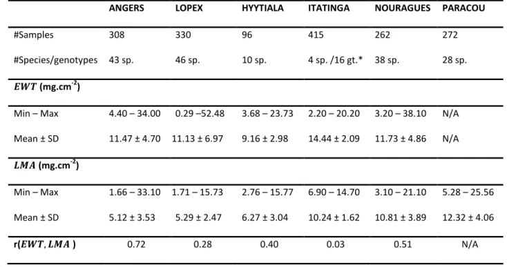
Table 1. Summary of the main properties of the experimental datasets. Basic statistics for each 288
dataset (minimum and maximum value, mean and standard deviation) are given for 𝑬𝑾𝑻 and 𝑳𝑴𝑨, 289
as well as their correlation r(𝑬𝑾𝑻, 𝑳𝑴𝑨). 290
ANGERS LOPEX HYYTIALA ITATINGA NOURAGUES PARACOU
#Samples 308 330 96 415 262 272
#Species/genotypes 43 sp. 46 sp. 10 sp. 4 sp. /16 gt.* 38 sp. 28 sp. 𝑬𝑾𝑻 (mg.cm-2)
Min – Max 4.40 – 34.00 0.29 –52.48 3.68 – 23.73 2.20 – 20.20 3.20 – 38.10 N/A Mean ± SD 11.47 ± 4.70 11.13 ± 6.97 9.16 ± 2.98 14.44 ± 2.09 11.73 ± 4.86 N/A 𝑳𝑴𝑨(mg.cm-2)
Min – Max 1.66 – 33.10 1.71 – 15.73 2.76 – 15.77 6.90 – 14.70 3.10 – 21.10 5.28 – 25.56 Mean ± SD 5.12 ± 3.53 5.29 ± 2.47 6.27 ± 3.04 10.24 ± 1.62 10.81 ± 3.89 12.32 ± 4.06
r(𝑬𝑾𝑻, 𝑳𝑴𝑨) 0.72 0.28 0.40 0.03 0.51 N/A
* Four species from Eucalyptus genus, corresponding to sixteen genotypes 291
292
3. METHODS 293
a. PROSPECT model: general presentation 294
PROSPECT is based on the generalized plate model (Allen et al., 1969, 1970) and was initially 295
developed by Jacquemoud and Baret (1990). This model simulates the leaf directional-hemispherical 296
14
reflectance and transmittance (Schaepman-Strub et al., 2006) with a limited number of input 297
biophysical and biochemical variables, including various absorbing compounds and a unique leaf 298
structure parameter, named 𝑁. Many versions have been developed since the first version, in order 299
to include more absorbing compounds (Féret et al., 2017, 2008; Jacquemoud et al., 1996) or to 300
adapt to specific conditions and leaf types, such as needle-shaped leaves (Malenovský et al., 2006). 301
In this study, we used the latest version of PROSPECT, named PROSPECT-D (Féret et al., 2017). As we 302
focused on leaf optical properties in the 900 – 2400 nm range, the capability of PROSPECT in terms 303
of separation of pigments was not critical as no pigment absorbs in this spectral domain, but the 304
refractive index differs from the one used on PROSPECT-5 (Féret et al., 2008). Brown pigments were 305
not retrieved during the inversion, as including them showed no significant difference in the results 306
obtained for any of the strategies tested here. 307
The 𝑁 parameter corresponds to the number of uniform compact plates separated by 𝑁 − 1 air 308
spaces. The value of 𝑁 represents the complexity of the leaf internal structure, with low 𝑁 values 309
corresponding to moderate complexity such as in monocots, and higher 𝑁 values corresponding to 310
higher complexity, a characteristic of dicots. To date, no protocol exists to experimentally estimate 311
𝑁 from leaf samples, other than using leaf optical properties. 𝑁 influences leaf scattering and shows 312
negligible impact on leaf absorption: increasing 𝑁 values increase reflectance and decrease 313
transmittance, and 𝑁 shows particularly strong effects in domains with low absorption, such as the 314
NIR domain. Recently, Qiu et al. (2018) found an extremely strong correlation between 𝑁 and the 315
ratio between reflectance and transmittance on simulated data. 316
PROSPECT can be run in forward or inverse mode. The forward mode aims at simulating leaf optical 317
properties based on a full set of biophysical and biochemical properties (leaf chemistry and 𝑁). The 318
inverse mode aims at identifying the optimal set of biophysical and biochemical properties that 319
minimize a merit function (or goodness-of-fit criterion) based on a comparison between measured 320
15
and simulated leaf optics. A common inversion procedure is based on the numerical minimization of 321
the sum of weighted square errors over all spectral bands available. The corresponding merit 322
function 𝑀 is expressed as follows when using both reflectance and transmittance: 323 324 𝑀(𝑁, { 𝐶𝑖}𝑖=1:𝑝) = ∑ [𝑊𝑅,𝜆× (𝑅𝜆− 𝑅̂𝜆)2+ 𝑊𝑇,𝜆× (𝑇𝜆− 𝑇̂𝜆)2] 𝜆𝑛 𝜆=𝜆1 Eq. 3 325
with 𝑁 the leaf structure parameter, 𝑝 the number of chemical constituents accounted for by 326
PROSPECT and retrieved during the inversion, 𝐶𝑖 the biochemical content per leaf surface unit for
327
constituent 𝑖, 𝜆1 and 𝜆𝑛 the first and last wavebands investigated for inversion, 𝑅𝜆 and 𝑇𝜆 the
328
experimental reflectance and transmittance measured at waveband 𝜆, 𝑅̂𝜆 and 𝑇̂𝜆 the reflectance and
329
transmittance simulated by PROSPECT with {𝑁, { 𝐶𝑖}𝑖=1:𝑝} as input variables, 𝑊𝑅,𝜆 the weight
330
applied to the squared difference between experimental and simulated reflectances, and 𝑊𝑇,𝜆 its
331
equivalent for transmittance. Eq. 3 can be used to estimate the full set of input variables, or a limited 332
subset if prior information or arbitrary value is set for some variables. 333
b. Estimation of 𝐸𝑊𝑇 and 𝐿𝑀𝐴 through iterative optimization 334
The large majority of the studies focusing on leaf scale model inversions through iterative 335
optimization used Eq. 3 with unweighted merit function over the full spectral domain available 336
(𝑊𝑅,𝜆= 𝑊𝑇,𝜆= 1).This merit function provides accurate estimates of leaf pigments and 𝐸𝑊𝑇 (Féret
337
et al., 2017; Jacquemoud et al., 1996; Newnham and Burt, 2001), but several studies reported poor 338
results for 𝐿𝑀𝐴 estimation (Féret et al., 2008; Riano et al., 2005). Colombo et al. (2008) used an 339
alternative weighting, with 𝑊𝑅,𝜆= (𝑅𝜆)−2 and 𝑊𝑇,𝜆= (𝑇𝜆)−2, which is otherwise unused in the
340
literature when inverting leaf models, and not so common when inverting canopy models (Baret and 341
Buis, 2008). In practice, implementing such a merit function requires precaution as high sensor noise 342
16
(in particular in the SWIR domain) may result in close-to-zero reflectance and transmittance, leading 343
to exaggerated importance of the corresponding spectral bands. This merit function then needs to 344
be adapted to exclude these spectral bands. Colombo et al. (2008) reported fair performances of this 345
merit function for the estimation of 𝐸𝑊𝑇, but poor performances for 𝐿𝑀𝐴. However, the SWIR 346
domain beyond 1600 nm was not measured for their study, in spite of its importance for the 347
estimation of 𝐿𝑀𝐴 (Asner et al., 2011, 2009; le Maire et al., 2008). Therefore a fair comparison 348
between this merit function and the unweighted merit function including the full spectral range is 349
required. 350
As mentioned in the introduction, 𝐿𝑀𝐴 estimation could also be improved by focusing on optimal 351
spectral ranges (Li and Wang, 2011; Qiu et al., 2018; Wang et al., 2015). This amounts to choosing 352
the weights such that 𝑊𝑅,𝜆= 𝑊𝑇,𝜆 = 1 in the considered range, and 𝑊𝑅,𝜆= 𝑊𝑇,𝜆 = 0 elsewhere.
353
Note that such a procedure is relatively straightforward and could potentially be applied to the 354
canopy scale in a similar way. 355
In this study, three inversion procedures were applied to the six independent experimental datasets, 356
and their relative performances were compared. These inversion procedures correspond to “one-357
step” procedures, aiming at estimating 𝐸𝑊𝑇, 𝐿𝑀𝐴 and 𝑁 simultaneously from both reflectance and 358
transmittance: 359
- Iterative optimization 1 (IO1) uses an unweighted merit function (𝑊𝑅,𝜆= 𝑊𝑇,𝜆 = 1) with
360
reflectance and transmittance defined from 900 nm to 2400 nm. 361
- Iterative optimization 2 (IO2) uses a weighted merit function as defined by Colombo et al. (2008) 362
(𝑊𝑅,𝜆= (𝑅𝜆)−2 and 𝑊𝑇,𝜆= (𝑇𝜆)−2) with reflectance and transmittance defined from 900 nm to
363
2400 nm. 364
- Iterative optimization 3 (IO3) uses a weighted merit function defined by 𝑊𝑅,𝜆= 𝑊𝑇,𝜆 = 1 over
365
an optimal contiguous spectral domain [𝜆1, 𝜆𝑛] defined between 900 and 2400 nm, and
17
𝑊𝑅,𝜆= 𝑊𝑇,𝜆= 0 elsewhere. This optimal spectral domain is adjusted in the present study and is
367
the same for both reflectance and transmittance, and for all experimental datasets. 368
In the case of IO3, the exhaustive comparison of all combinations of spectral domains or spectral 369
bands is computationally too demanding and extremely inefficient given the strong correlations 370
between neighboring spectral domains. In order to reduce the computational cost, we focused on 371
contiguous spectral domains defined by partitioning the initial spectral domain into 15 evenly-sized 372
segments of 100 nm from 900 to 2399 nm. The choice of 100 nm segments is driven by constraints in 373
terms of computation and by the ability to identify the main absorption features of 𝐸𝑊𝑇 and 𝐿𝑀𝐴 374
individually. The performances of PROSPECT inversion for the estimation of 𝐿𝑀𝐴 and 𝐸𝑊𝑇 were 375
tested with all continuous spectral domains that can be generated from these 15 spectral segments, 376
leading to 120 continuous segments. Finally, the spectral domain leading to the minimum RMSE 377
averaged for all experimental datasets and for the estimation of both 𝐿𝑀𝐴 and 𝐸𝑊𝑇 from 378
PROSPECT inversion was selected and defined as the optimal spectral range used in IO3. 379
For IO1, IO2 and IO3, 𝑁, 𝐸𝑊𝑇 and 𝐿𝑀𝐴 were simultaneously estimated using a constrained 380
nonlinear optimization algorithm, i.e., the Sequential Quadratic Programming algorithm 381
implemented within the Matlab function fmincon. The lower bounds selected for the three 382
parameters to be optimized were defined to respect the condition of strict positivity and include 383
minimum values observed for experimental data, whereas the upper bounds were set in order to 384
include the maximum values observed for experimental data, with significant margins: 𝐸𝑊𝑇 values 385
were investigated between 0.01 and 80 mg.cm-2; 𝐿𝑀𝐴 values were investigated between 0.01 and 386
40 mg.cm-2; 𝑁 values were investigated between 0.5 and 4. No correlation constraints between 387
𝐸𝑊𝑇 and 𝐿𝑀𝐴 were included in the inversion procedure, since such correlation was not systematic 388
between datasets. 389
18 c. Data-driven estimation of 𝐸𝑊𝑇 and 𝐿𝑀𝐴 391
The performances of data-driven methods inherently depend on the training data. In most cases, 392
these performances are reported after splitting an experimental dataset into training and validation 393
subsets, and the resulting regression models are not validated on fully independent datasets. In the 394
perspective of operational applications, this raises the question of the possibility to share regression 395
models adjusted with ML algorithms on public experimental datasets, and to use leaf spectroscopy 396
operationally with no destructive measurements required to adjust dataset-specific regression 397
models. With increasing use of machine learning, software packages including already trained 398
regression models may be shared the same way statistical models derived from spectral indices have 399
been proposed in the scientific literature (Féret et al., 2011). We want to answer the following 400
questions related to data-driven methods: do regression models trained with one or several 401
experimental datasets perform well when applied on independent datasets, or should training data 402
systematically include samples from the validation dataset? To answer these questions, three 403
strategies for the composition of a training dataset were tested, and the performances of data-404
driven methods were compared with PROSPECT inversions: 405
- Training sampling 1 (TS1): A single dataset was used as training data and the regression model 406
was then applied on each of the remaining datasets. 407
- Training sampling 2 (TS2): All but one experimental datasets were used as training data, and the 408
regression model was then applied on the remaining dataset. 409
- Training sampling 3 (TS3): All experimental datasets were pooled into a single one, and 300 410
samples (comparable in size to individual datasets) were randomly selected for training. 411
Validation was then performed on the remaining samples (1668 samples for 𝐿𝑀𝐴, and 1396 412
samples for 𝐸𝑊𝑇), and performances (in terms of RMSE) were evaluated per individual dataset 413
and globally. In each case, to account for possible sampling bias, random sampling of training 414
19
dataset was repeated 20 times and the distribution of RMSE values across all samplings was 415
calculated. 416
Here, these three strategies used to define the training dataset were used with support vector 417
machine (SVM) regression algorithm corresponding to the Matlab implementation of the LibSVM 418
library (Chang and Lin, 2011). Reflectance and transmittance measurements from 900 to 2400 nm 419
were stacked in a unique vector, resulting in 𝑛𝜆= 3002 predictor spectral variables for each sample.
420
Reflectance and transmittance were scaled between 0 and 1 for each spectral band, as well as leaf 421
chemical constituent of interest (𝐿𝑀𝐴 and 𝐸𝑊𝑇). The radial basis function (RBF) kernel was 422
selected, which implies optimizing two free parameters, 𝐶 and 𝛾. 𝐶 is a cost parameter used to trade 423
error penalty for stability and common to any SVM model. 𝛾 is specific to RBF kernels and it 424
corresponds to the inverse of the radius of influence of samples selected by the model as support 425
vectors. The 𝐶 and 𝛾 parameters were optimized using an exhaustive grid search 426
(𝐶 ∈ [10−2; 10−1; … ; 10+2], 𝛾 ∈ [10−5; 10−4; … ; 10+1] in order to include the default values 427
recommended by Chang and Lin (2011) and a five-fold cross validation over the training data for 428
each combination of 𝐶 and 𝛾. The optimal 𝐶 and 𝛾 values were then used with the full training data 429
to adjust a regression model. 430
431
4. RESULTS 432
This section is divided into three subsections. The first subsection aims at identifying the optimal 433
spectral domain to be used with IO3. This first section is a prerequisite to the second section, which 434
then focuses on the comparison between the three types of iterative optimization, and the two 435
types of training samplings based on the integrality of experimental datasets, TS1 and TS2. Finally, 436
the third section compares the performances of TS3, which is based on a random sampling among all 437
20
experimental datasets, with the performances of IO3 and TS2, when the validation samples are 438
identical to those used in TS3. 439
a. Influence of spectral domain used for the estimation of 𝐸𝑊𝑇 and 𝐿𝑀𝐴 with 440
PROSPECT inversion (optimization of IO3 method) 441
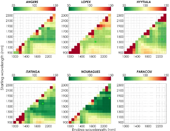
Figure 1 and Figure 2 show the results obtained for the estimation of 𝐸𝑊𝑇 and 𝐿𝑀𝐴, respectively, 442
when inverting PROSPECT over each dataset and each of the 120 spectral domains defined in Section 443
3.b with the IO3 method. For the sake of comparison, for each dataset, the RMSE was normalized by 444
the RMSE obtained when using the spectral information from 900 to 2400 nm, and this normalized 445
RMSE (NRMSE) was expressed as a percentage. In the case of 𝐸𝑊𝑇, the optimal spectral domain 446
excluded the NIR domain under 1300 nm for all datasets, but no unique optimal spectral domain 447
common to each dataset could be identified. The relative improvement induced by the reduction of 448
the spectral domain was also strongly dataset-dependent: NRMSE was reduced by 23 % (LOPEX) to 449
56 % (NOURAGUES). 450
21
Figure 1. Normalized 𝑅𝑀𝑆𝐸 (𝑁𝑅𝑀𝑆𝐸, in %) obtained for 𝐸𝑊𝑇 with PROSPECT inversion method IO3 over each dataset and each reduced spectral domains bounded by a starting wavelength 𝜆1 (y-axis)
and an ending wavelength 𝜆2 (x-axis). The normalization is specific to each dataset based on the
performances of IO1 (NRMSE=100%, lower right corner). The green star indicates the spectral segment producing the best results.
451
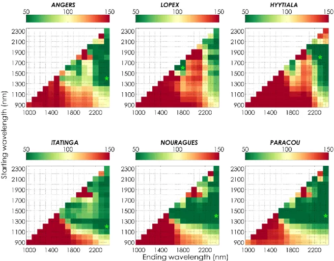
In the case of 𝐿𝑀𝐴, both optimal spectral domain and relative improvement or degradation showed 452
stronger consistency among datasets than for 𝐸𝑊𝑇 (Figure 2). For all datasets, excluding 453
information from 1500 nm and beyond led to strong degradations of the performances. In the case 454
22
of LOPEX and HYYTIALA, estimation of 𝐿𝑀𝐴 could be improved only when using spectral domains 455
with ending wavelength between 2100 and 2400 nm, except when using a narrow spectral domain 456
from 1600 to 1800 nm. For the four other datasets, extended spectral combinations led to improved 457
𝐿𝑀𝐴, as most of the combinations excluding the domain from 900 to 1200 nm led to improved 458
estimation of 𝐿𝑀𝐴, except when using a reduced spectral domain ranging from 1800 to 2100 nm 459
only, which corresponds to one of the main absorption features of water. Overall, the optimal 460
spectral range excluded the NIR domain and included spectral information until 2400 nm for all 461
datasets. The relative improvement induced by the selection of an optimal specific for each dataset 462
ranged from 60 (ITATINGA) to 67 % (NOURAGUES). 463
23
Figure 2. Normalized 𝑅𝑀𝑆𝐸 (NRMSE, in %) obtained for 𝐿𝑀𝐴 estimation with PROSPECT inversion method IO3, over each dataset and each reduced spectral domains bounded by a starting wavelength 𝜆1 (y-axis) and an ending wavelength 𝜆2 (x-axis). The normalization is specific to each
dataset based on the performances of IO1 (NRMSE=100%, lower right corner). The green star indicates the spectral segment producing the best results.
465
These figures provide a visual representation of the spectral domains leading to improved or 466
decreased performances compared to full spectral information. They confirm that selecting the 467
appropriate spectral information during inversion strongly influences for the estimation of leaf 468
constituents. 469
24
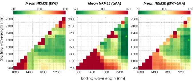
Figure 3 provides NRMSE for the estimation of 𝐸𝑊𝑇 and 𝐿𝑀𝐴 averaged over all datasets, and 470
confirms suboptimal performances obtained when using NIR information only. Overall, the spectral 471
domain ranging from 1700 to 2400 nm was found to be optimal when estimating 𝐸𝑊𝑇 and 𝐿𝑀𝐴 472
simultaneously (mean NRMSE was reduced by 33% for 𝐸𝑊𝑇 and by 55 % for 𝐿𝑀𝐴), and was used 473
hereafter within the IO3 method. 474
475
Figure 3. Mean normalized RMSE values (NRMSE, in %) obtained for the estimation of 𝐸𝑊𝑇 (left), 𝐿𝑀𝐴 (center), and both constituents (right), after PROSPECT inversion over all experimental datasets
pooled and each of the 120 spectral domains defined in Section 3.b. The green star indicates the spectral segment producing the best results.
476
b. Comparison of PROSPECT inversion methods and ML algorithms for the estimation 477
of 𝐿𝑀𝐴 and 𝐸𝑊𝑇: training ML with independent datasets 478
The performances obtained for the estimation of 𝐸𝑊𝑇 when using TS1 and TS2 for ML regression, 479
and IO1, IO2 or IO3 (with the 1700 – 2400 nm spectral range) for PROSPECT inversion are reported in 480
Table 2. Overall, IO2 and IO3 produced the most consistent results, systematically outperforming the 481
25
other methods. ML regressions performed particularly poorly compared to IO2 and IO3, and TS2 led 482
to the better results than TS1 (except form HYYTIALA). TS1 led to very inconsistent results, with 483
175% increase compared to IO2 and IO3 on average, and up to 500% increase in RMSE compared to 484
PROSPECT inversion IO2 when estimating 𝐸𝑊𝑇 from ITATINGA after training with LOPEX. 485
486
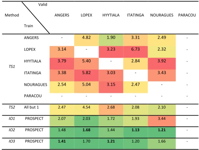
Table 2. RMSE values (in mg.cm-2) obtained for the estimation of 𝐸𝑊𝑇 with SVM and training 487
strategies TS1 and TS2, and with IO1, IO2 and IO3. For each column (validation dataset), the 488
minimum RMSE is indicated in bold, and colors correspond to the level of performances, from green 489
color for minimum RMSE to red color for maximum RMSE. 490
Method
Valid
Train
ANGERS LOPEX HYYTIALA ITATINGA NOURAGUES PARACOU
TS1 ANGERS - 4.82 1.90 3.31 2.49 - LOPEX 3.14 - 3.23 6.73 2.32 - HYYTIALA 3.79 5.40 - 2.84 3.92 - ITATINGA 3.38 5.82 3.03 - 3.43 - NOURAGUES 2.54 5.04 3.15 2.47 - - PARACOU - - - - TS2 All but 1 2.47 4.54 2.68 2.08 2.10 - IO1 PROSPECT 2.07 2.03 1.72 1.93 3.44 - IO2 PROSPECT 1.48 1.68 1.44 1.13 1.21 - IO3 PROSPECT 1.41 1.70 1.21 1.20 1.66 - 491
26
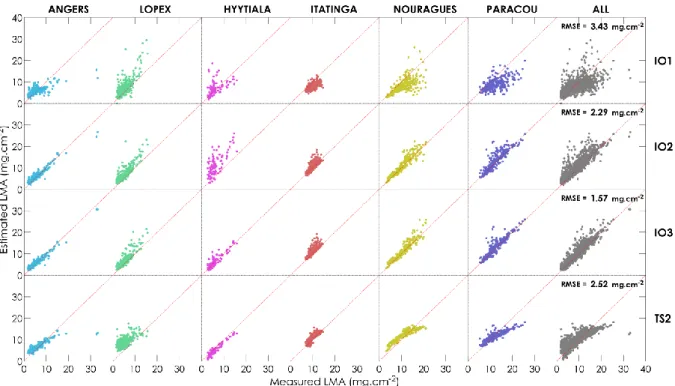
Figure 4 provides scatterplots for the results showed in Table 2 and corresponding to IO1, IO2, IO3 492
and SVM regression with sampling strategy TS2. Overall, IO2 showed the best performances for the 493
estimation of 𝐸𝑊𝑇, and SVM regression produced the lowest performances, mainly because of the 494
strong error obtained for extreme values on LOPEX. 495
496
Figure 4. 𝐸𝑊𝑇 estimation results obtained using PROSPECT inversion (IO1, IO2, IO3) and ML regression (training sampling TS2).
497
The performances obtained for the estimation of 𝐿𝑀𝐴 when using training samplings TS1 and TS2 498
for ML regression, and IO1, IO2 or IO3 for PROSPECT inversion are reported in Table 3. IO3 499
outperformed the other methods for all datasets except HYYTIALA and ITATINGA: IO2 slightly 500
outperformed IO3 for ITATINGA only and TS2 outperformed IO3 for HYYTIALA and ITATINGA. 501
However, the difference in RMSE between IO3 and the optimal method remained less than 20% for 502
these two datasets. The relative performances obtained with IO1 and IO2 differed among datasets: 503
27
while using IO2 led to significantly improved estimation of 𝐿𝑀𝐴 compared to IO1 for five datasets 504
(from a 26% decrease in RMSE for LOPEX to more than 50% for ITATINGA, NOURAGUES and 505
PARACOU), and slightly degraded estimation compared to IO3 for four datasets, the performances 506
obtained for HYYTIALA were degraded by more than 75% compared to IO1, with systematic strong 507
overestimation (Figure 5). On the other hand, the RMSE corresponding to estimation of 𝐿𝑀𝐴 using 508
IO3 decreased by 60% compared to IO1. ML regression trained with TS2 performed better than IO1 509
overall but was outperformed by IO2 and IO3. As for 𝐸𝑊𝑇, ML trained with TS1 led to very 510
inconsistent results, and was strongly outperformed by IO2, IO3 and ML regressions trained with 511
strategy TS2 in most cases. 512
513
Table 3. RMSE values (in mg.cm-2) obtained for the estimation of 𝐿𝑀𝐴 with SVM and training 514
samplings TS1 and TS2, and with IO1, IO2 and IO3. For each column (validation dataset), the 515
minimum RMSE is indicated in bold, and colors correspond to the level of performances, from green 516
color for minimum RMSE to red color for maximum RMSE. 517
Method
Valid
Train
ANGERS LOPEX HYYTIALA ITATINGA NOURAGUES PARACOU
TS1 ANGERS - 4.91 2.49 3.73 2.76 2.70 LOPEX 2.92 - 2.18 4.33 4.85 5.86 HYYTIALA 2.51 2.47 - 3.19 3.32 4.00 ITATINGA 6.27 5.57 5.08 - 3.86 4.50 NOURAGUES 4.04 4.82 3.74 1.40 - 2.21 PARACOU 2.96 3.96 2.30 1.25 2.11 - TS2 All but 1 2.31 4.06 1.33 1.23 2.14 2.41
28
IO1 PROSPECT 2.48 3.36 3.49 2.60 3.95 4.75
IO2 PROSPECT 1.24 2.48 6.12 1.20 1.71 2.25
IO3 PROSPECT 0.93 1.99 1.52 1.44 1.59 1.73
518
Figure 5 provides scatterplots for the results showed in Table 3 and corresponding to IO1, IO2, IO3 519
and SVM regression with training sampling TS2. Overall, IO3 produced the most accurate estimation 520
of 𝐿𝑀𝐴. IO2, IO3 and TS2 respectively resulted in 33%, 55% and 27% decreases in RMSE for the 521
estimation of 𝐿𝑀𝐴 when compared to IO1. 522
523
Figure 5. 𝐿𝑀𝐴 estimation results obtained using PROSPECT inversion (IO1, IO2, IO3) and SVM regression (training sampling TS2).
29
c. Comparison of PROSPECT inversion methods and ML algorithms for the estimation 525
of 𝐿𝑀𝐴 and 𝐸𝑊𝑇: training ML with pooled datasets 526
Table 4 and Table 5 summarize the performances of SVM regression for the estimation of 𝐸𝑊𝑇 and 527
𝐿𝑀𝐴 when TS3 is selected as training strategy (i.e. all dataset are pooled together and 300 528
calibration samples are randomly selected). The performances corresponding to IO3 and TS2 were 529
computed for the same validation samples as with TS3 for each of the 20 repetitions in order to 530
ensure fair comparison. 531
The mean performances reported in Table 4 and Table 5 were very similar to those reported in Table 532
2 and Table 3 for both IO3 and TS2, which means that IO3 systematically outperformed TS2 on 533
individual datasets, except for the estimation of 𝐿𝑀𝐴 for HYYTIALA and ITATINGA. TS3 534
outperformed TS2 in most cases for the estimation of both 𝐸𝑊𝑇 and 𝐿𝑀𝐴. Still, TS3 was 535
outperformed by IO3 when estimating 𝐸𝑊𝑇, the overall RMSE increasing by 44% (and by 99% when 536
using TS2). When estimating 𝐿𝑀𝐴, TS3 and IO3 showed very similar overall performances, with less 537
than 6% increase of RMSE for TS3 when compared to IO3. IO3 and TS3 showed very similar average 538
RMSE for LOPEX, HYTTIALA and NOURAGUES, TS3 showed higher RMSE for ANGERS and PARACOU, 539
and lower RMSE for ITATINGA. However, the standard deviations associated with these 540
performances highlight the strong effect of training and validation samplings on the performances of 541
the ML algorithm: the standard deviation computed over 20 repetitions was 5 to 20 times higher for 542
TS3 than IO3 when estimating 𝐸𝑊𝑇, while it was 2.5 to 10 times higher when estimating 𝐿𝑀𝐴. The 543
standard deviations related to the performances of TS2 were generally similar to those obtained for 544
IO3, suggesting that the strong differences in performance between regression models were induced 545
by the selection of the training samples. 546
30
Table 4. Mean RMSE and standard deviation of RMSE (both in mg.cm-2) of the estimation of 𝐸𝑊𝑇 548
using SVM regression (TS2 and TS3) and PROSPECT inversion (IO3) on the validation samples used for 549
TS3. Best mean performances are indicated in bold. 550
ANGERS LOPEX HYYTIALA ITATINGA NOURAGUES PARACOU Total
TS3 1.76±0.24 2.77±0.47 2.08±0.37 1.64±0.33 2.18±0.37 - 2.12±0.26 TS2 2.47±0.04 4.55±0.28 2.66±0.07 2.08±0.04 2.1±0.05 - 2.97±0.10 IO3 1.43±0.04 1.70±0.07 1.21±0.04 1.21±0.02 1.65±0.05 - 1.47±0.02 551
Table 5. Mean RMSE and standard deviation of RMSE (both in mg.cm-2) of the estimation of 𝑳𝑴𝑨 552
using SVM regression (TS2 and TS3) and PROSPECT inversion (IO3) on the validation samples used for 553
TS3. Best mean performances are indicated in bold (differences in mean RMSE < 1% are considered 554
equivalent). 555
ANGERS LOPEX HYYTIALA ITATINGA NOURAGUES PARACOU Total
TS3 1.70±0.28 1.98±0.56 1.56±0.22 1.12±0.29 1.59±0.19 2.01±0.18 1.64±0.18 TS2 2.24±0.21 4.05±0.06 1.33±0.04 1.23±0.02 2.13±0.03 2.43±0.05 2.31±0.05 IO3 0.92±0.03 2.00±0.07 1.54±0.08 1.45±0.04 1.58±0.06 1.77±0.07 1.54±0.03 556 5. DISCUSSION 557
a. Differences in performances among merit functions 558
Our study shows that IO1, the most commonly used merit function, is actually outperformed by a 559
less common merit function (IO2) when estimating 𝐸𝑊𝑇 and 𝐿𝑀𝐴 from PROSPECT inversion using 560
reflectance and transmittance in the NIR/SWIR domain (900-2400 nm). These results are in 561
agreement with the results obtained when investigating the optimal spectral domain to be used with 562
31
IO3: Figure 3 shows that, in most cases, selecting a spectral domain including NIR information leads 563
to suboptimal estimation of both 𝐸𝑊𝑇 and 𝐿𝑀𝐴. Therefore, the application of a weight inversely 564
proportional to the square of the reflectance and transmittance (IO2) reduce the importance of 565
spectral domains showing higher reflectance and transmittance values such as the NIR domain. The 566
improvement is particularly strong for the estimation of 𝐿𝑀𝐴, as reported in Figure 3. The 567
particularly low performances obtained for the estimation of 𝐿𝑀𝐴 on HYYTIAA were also 568
investigated. The leaf optical properties measured for this dataset showed low SNR, particularly in 569
the SWIR domain for wavelengths of 2300 nm and beyond. The estimation of 𝐿𝑀𝐴 with IO2 was 570
strongly improved on this dataset when applying a Savitzky-Golay smoothing filter and restricting 571
the spectral domain from 1700 to 2300 nm. The exclusion of the spectral domain beyond 2300 nm 572
was responsible for the strongest improvement. Finally, the RMSE obtained for HYYTIAA when using 573
the merit function used in IO2 and these preprocessing reached 1.97 mg.cm-2, which is still 30% 574
higher than the RMSE obtained with IO3. Therefore using IO2 is strongly discouraged when the 575
signal to noise ratio of leaf optical properties is not sufficient, while IO3 based on the 1700-2400 nm 576
spectral range appears to be reliable even with low SNR. 577
578
b. Physical interpretation of the performances obtained with PROSPECT inversion 579
As highlighted in the previous section, the SNR of leaf optical properties can become a strong 580
limitation when estimating leaf constituents using PROSPECT inversion if the spectral domain and 581
merit functions are not carefully chosen. However, this SNR is not the main limiting factor explaining 582
the poor performances of IO1 for the estimation of 𝐿𝑀𝐴 and its suboptimal performances for the 583
estimation of 𝐸𝑊𝑇. Indeed, the NIR domain is theoretically characterized by a higher signal to noise 584
ratio for leaf material but still appears to be the main limitation for an accurate estimation of these 585
32
leaf constituents. Therefore, we attempt here to list possible explanations for such poor 586
performances. 587
i. Predominant water absorption 588
The main reason cited to explain the poor retrieval of 𝐿𝑀𝐴 is the predominant water absorption in 589
the SWIR domain. Indeed, Figure 3 Erreur ! Source du renvoi introuvable.shows that 𝐿𝑀𝐴 is poorly 590
estimated when the spectral domains used for inversion mainly include domains with strong water 591
absorption, such as the domain from 1800 to 2100 nm. However Figure 3 also shows that 𝐿𝑀𝐴 can 592
still be estimated accurately even if most of the spectral information corresponds to domains with 593
predominant water absorption. Our results show that the main limitation with IO1 is actually caused 594
by the NIR domain between 900 and 1300 nm: most of the spectral domains excluding such 595
wavebands resulted in improved estimation of 𝐿𝑀𝐴. The 900-1300 nm range does not show 596
predominant water or dry matter absorption, so the poor retrieval of 𝐿𝑀𝐴 cannot be explained by 597
absorption features hidden by water absorption or any other constituent. 598
ii. Approximations of PROSPECT 599
As any model, PROSPECT is based on a number of approximations. Although some of these 600
approximations are possible sources of inaccuracy in specific situations, they guarantee good overall 601
performances given a minimum number of descriptors of leaf biophysical properties. Model 602
discrepancies in the simulation of leaf optical properties may be explained by inaccurate physical 603
description at three levels: surface effects, volume scattering and volume absorption. 604
Surface effects strongly depend on the presence of waxes or trichomes, and Barry and Newnham 605
(2012) reported how epicuticular waxes affect PROSPECT inversion. Surface effects mostly influence 606
leaf reflectance in the domains characterized by strong absorption where the leaf reflectance is 607
minimum (Bousquet et al., 2005; Jay et al., 2016). In the NIR/SWIR spectral range, these domains 608
mainly depend on water absorption. The sensitivity analysis performed by Jay et al. (2016) with 609
33
similar 𝐸𝑊𝑇 values showed that surface effects have the largest influence beyond 1800 nm, this 610
domain being close to the one leading to optimal PROSPECT inversion results with IO3 (1700-2400 611
nm). Such a result thus tends to indicate that surface effects had a limited detrimental influence on 612
estimation performance. 613
Volume scattering is modeled by multiple factors in PROSPECT, including leaf structure with the 𝑁 614
parameter, and the refractive index. The unique value of the refractive index is a well-identified 615
simplification of PROSPECT, as it does not agree with the Kramers-Kronig relations stating that the 616
real (refractive index) and imaginary (absorption coefficient) parts of the complex refractive index of 617
a medium are physically linked (Lucarini et al., 2005). Qiu et al. (2018) developed PROSPECT-g, a 618
modified version of PROSPECT including an additional wavelength-independent factor specific to 619
each leaf and aiming at representing first-order effects of anisotropic scattering, which are not 620
included through the N structural parameter of the original PROSPECT model. They also proposed a 621
multistage inversion to be used with PROSPECT-g. This inversion procedure may strongly increase 622
computing time, and the applicability of PROSPECT-g inversion at the canopy scale does not seem 623
straightforward as additional parameters may increase the ill-posedness of canopy models such as 624
PROSAIL (Jacquemoud et al., 2009). However, they reported promising results, including improved 625
estimation of 𝐿𝑀𝐴 and improved simulation of both reflectance and transmittance in the NIR 626
domain when compared to PROSPECT-5. 627
Volume absorption is defined by the SACs which are adjusted based on experimental data during the 628
calibration of PROSPECT (Féret et al., 2008, 2017). We attempted a recalibration of the SAC for 𝐿𝑀𝐴 629
in order to reduce the inaccuracies observed between experimental and simulated data, and 630
improve the estimation of 𝐿𝑀𝐴. This did not lead to any improvement when including the NIR 631
domain. Moreover, the incorrect definition of the SAC corresponding to 𝐿𝑀𝐴 would lead to 632
systematic underestimation or overestimation of absorption when running PROSPECT in direct 633
34
mode. However, the analysis of the residuals between measured leaf optical properties and their 634
simulated counterparts obtained with PROSPECT in direct mode did not result in systematic errors 635
(results not shown). The SAC corresponding to 𝐿𝑀𝐴 in PROSPECT integrates the optical influences of 636
various organic constituents, which may also lead to inaccuracies if leaf samples include strong 637
variations in stoichiometry. However, the data required to test this possible source of inaccuracy 638
was not available. 639
iii. Bias in the leaf optical measurements 640
As highlighted in the introduction, the uncertainty associated to leaf optical measurements in the 641
NIR domain may be increased because of the incomplete collection of the light leaving the highly 642
scattering tissue (Merzlyak et al., 2002). Merzlyak et al. (2004) proposed a correcting factor for 643
transmittance based on the hypothesis that leaf absorption in the NIR domain from 780 to 900 nm is 644
negligible for healthy leaves. However this correcting factor is not adopted as a standard correction 645
by the community. In order to detect possible uncertainty in the optical measurements in the NIR 646
domain with our data, we tested our ML approach with TS1 (training with a unique dataset) and 647
spectral information either from 1700 to 2400 nm or from 1400 to 2400 nm (results not showed). 648
For both 𝐿𝑀𝐴 and 𝐸𝑊𝑇, the regression models applied on independent datasets performed 649
similarly for the two spectral domains considered, but systematically performed better than the 650
regression models trained with the spectral information from 900 to 2400 nm. However, they were 651
still outperformed by PROSPECT inversion. Such a result thus tends to confirm that leaf optical 652
measurements in the NIR domain might be affected by some experimental uncertainty. 653
The poor performances reported for the estimation of 𝐿𝑀𝐴 with PROSPECT inversion using IO1 are 654
therefore mainly explained by the use of the NIR domain, which is subject to inaccuracies, from a 655
modeling and/or from an experimental point of view. Based on our study, we cannot conclude on 656
the relative importance of one or the other factor. These two possibilities should then be considered 657