HAL Id: hal-02894987
https://hal-ifp.archives-ouvertes.fr/hal-02894987v2
Submitted on 15 Sep 2020
HAL is a multi-disciplinary open access
archive for the deposit and dissemination of
sci-entific research documents, whether they are
pub-lished or not. The documents may come from
teaching and research institutions in France or
abroad, or from public or private research centers.
L’archive ouverte pluridisciplinaire HAL, est
destinée au dépôt et à la diffusion de documents
scientifiques de niveau recherche, publiés ou non,
émanant des établissements d’enseignement et de
recherche français ou étrangers, des laboratoires
publics ou privés.
Distributed under a Creative Commons Attribution| 4.0 International License
Addressing temporal considerations in life cycle
assessment
Didier Beloin-Saint-Pierre, Ariane Albers, Arnaud Hélias, Ligia Tiruta-Barna,
Peter Fantke, Annie Levasseur, Enrico Benetto, Anthony Benoist, Pierre
Collet
To cite this version:
Didier Beloin-Saint-Pierre, Ariane Albers, Arnaud Hélias, Ligia Tiruta-Barna, Peter Fantke, et al..
Addressing temporal considerations in life cycle assessment. Science of the Total Environment,
Else-vier, 2020, 743, pp.140700. �10.1016/j.scitotenv.2020.140700�. �hal-02894987v2�
Review
Addressing temporal considerations in life cycle assessment
Didier Beloin-Saint-Pierre
a,⁎
, Ariane Albers
b, Arnaud Hélias
c, Ligia Tiruta-Barna
d, Peter Fantke
e,
Annie Levasseur
f, Enrico Benetto
g, Anthony Benoist
h, Pierre Collet
ba
Empa Materials Science and Technology, Lerchenfeldstrasse 5, CH-9014 St. Gallen, Switzerland b
IFP Energies Nouvelles, 1 et 4 Avenue de Bois-Préau, 92852 Rueil-Malmaison, France c
ITAP, Irstea, Montpellier SupAgro, Univ Montpellier, ELSA Research Group, Montpellier, France d
TBI, Université de Toulouse, CNRS, INRAE, INSA, Toulouse, France e
Quantitative Sustainability Assessment, Department of Technology, Management and Economics, Technical University of Denmark, Kgs. Lyngby, Denmark fÉcole de technologie supérieure, Construction Engineering Department, 1100 Notre-Dame West, Montréal, Québec, Canada
g
Environmental Sustainability Assessment and Circularity Unit, Department of Environmental Research and Innovation, Luxembourg Institute of Science and Technology, Esch/Alzette, Luxembourg h
CIRAD, UPR BioWooEB, F-34398 Montpellier, France
H I G H L I G H T S
• Review of temporal considerations in the life cycle assessment methodology • Glossary of important terms for time
considerations in life cycle assessment • Key aspects of dynamic life cycle
assess-ments
• Current implementation challenges for dynamic life cycle assessment • Development pathways for future
dy-namic life cycle assessment
G R A P H I C A L A B S T R A C T
a b s t r a c t
a r t i c l e i n f o
Article history:
Received 18 February 2020 Received in revised form 5 June 2020 Accepted 1 July 2020
Available online 9 July 2020 Editor: Deyi Hou Keywords: Dynamic LCA Temporal considerations Review Recommendations Implementation challenges
In life cycle assessment (LCA), temporal considerations are usually lost during the life cycle inventory calculation, resulting in an aggregated“snapshot” of potential impacts. Disregarding such temporal considerations has previ-ously been underlined as an important source of uncertainty, but a growing number of approaches have been de-veloped to tackle this issue. Nevertheless, their adoption by LCA practitioners is still uncommon, which raises concerns about the representativeness of current LCA results. Furthermore, a lack of consistency can be observed in the used terms for discussions on temporal considerations. The purpose of this review is thus to search for common ground and to identify the current implementation challenges while also proposing development pathways.
This paper introduces a glossary of the most frequently used terms related to temporal considerations in LCA to build a common understanding of key concepts and to facilitate discussions. A review is also performed on cur-rent solutions for temporal considerations in diffecur-rent LCA phases (goal and scope definition, life cycle inventory analysis and life cycle impact assessment), analysing each temporal consideration for its relevant conceptual de-velopments in LCA and its level of operationalisation.
We then present a potential stepwise approach and development pathways to address the current challenges of implementation for dynamic LCA (DLCA). Three key focal areas for integrating temporal considerations within the LCA framework are discussed: i) define the temporal scope over which temporal distributions of emissions
⁎ Corresponding author.
E-mail address:[email protected](D. Beloin-Saint-Pierre).
https://doi.org/10.1016/j.scitotenv.2020.140700
0048-9697/© 2020 The Authors. Published by Elsevier B.V. This is an open access article under the CC BY license (http://creativecommons.org/licenses/by/4.0/).
Contents lists available atScienceDirect
Science of the Total Environment
j o u r n a l h o m e p a g e :w w w . e l s e v i e r . c o m / l o c a t e / s c i t o t e n vare occurring, ii) use calendar-specific information to model systems and associated impacts, and iii) select the appropriate level of temporal resolution to describe the variations offlows and characterisation factors. Addressing more temporal considerations within a DLCA framework is expected to reduce uncertainties and in-crease the representativeness of results, but possible trade-offs between additional data collection efforts and the increased value of results from DLCAs should be kept in mind.
© 2020 The Authors. Published by Elsevier B.V. This is an open access article under the CC BY license (http:// creativecommons.org/licenses/by/4.0/).
Contents
1. Introduction . . . 2
2. Proposed glossary . . . 3
3. Temporal considerations for different purposes . . . 3
3.1. Phase of goal and scope definition . . . 4
3.1.1. Modelling choices . . . 4
3.1.2. Data quality requirements (DQR) . . . 4
3.1.3. Chosen limits of assessment . . . 6
3.2. Phase of inventory analysis: system modelling. . . 7
3.2.1. Inherent variations withflow differentiation . . . 7
3.2.2. Temporal resolution . . . 7
3.2.3. Modelling evolutions with process differentiation . . . 7
3.2.4. Prospective modelling . . . 7
3.3. Phase of inventory analysis: LCI computation . . . 8
3.3.1. Computational framework . . . 8
3.3.2. Approaches and tools . . . 8
3.4. Phase of life cycle impact assessment . . . 9
3.4.1. Modelling choices . . . 9
3.4.2. Chosen limits of assessment . . . 10
3.4.3. Temporal indicator . . . 10
3.4.4. Inherent variations . . . 10
3.4.5. Temporal resolution . . . 10
3.4.6. Modelling evolutions . . . 11
3.4.7. Strategies for prospective modelling . . . 11
3.4.8. Computational framework . . . 11
3.4.9. Approach and tools . . . 11
4. Proposed development pathways . . . 11
4.1. Stepwise approach for temporal considerations with current knowledge . . . 12
4.2. Temporal considerations in the goal and scope definition . . . 12
4.3. Time dependent modelling of human activities . . . 12
4.4. Inventory calculation: keeping time in the LCI . . . 14
4.5. Dynamics of impact assessment . . . 14
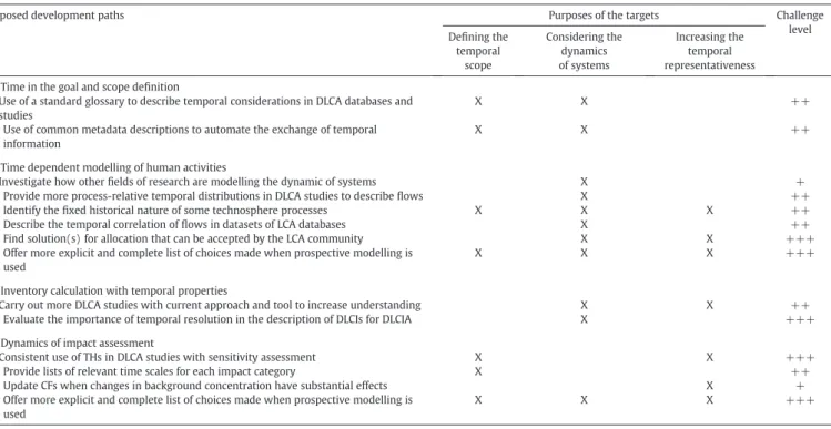
4.6. Summary of potential development paths for temporal considerations in DLCA . . . 15
5. Conclusions. . . 15
Declaration of competing interest . . . 16
Acknowledgements . . . 16
References. . . 16
1. Introduction
Disregarding temporal considerations1has been identified as an
in-herent limitations of life cycle assessment (LCA) (ISO14040, 2006; ISO14044, 2006). Indeed, the importance of properly considering the dynamics of environmental sustainability for the comparison of prod-ucts, services or systems has been explored, debated and confirmed during the last 20 years by many researchers likeOwens (1997a), Herrchen (1998),Reap et al. (2008a, 2008b),Finnveden et al. (2009), Levasseur et al. (2010)andMcManus and Taylor (2015), to name a few. In this discussion,Rebitzer et al. (2004),Reap et al. (2008a)and Yuan et al. (2015)have mainly explored the subject of dynamics in human activities. During the same period,Reap et al. (2008b),Shah and Ries (2009),Fantke et al. (2012),Kendall (2012),Levasseur et al.
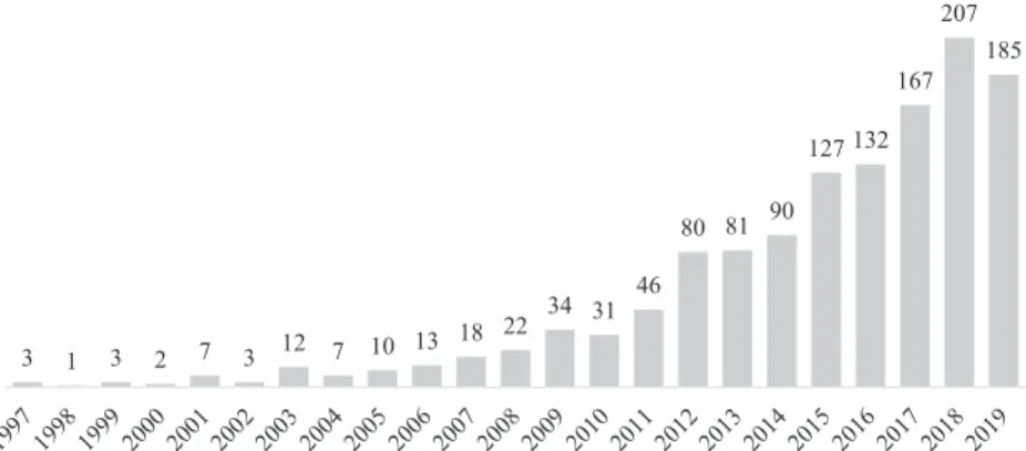
(2012b)andManneh et al. (2012)have proposed different ideas on the dynamics of environmental responses to human pressures. Addi-tionally,Hellweg et al. (2003b, 2005), Hellweg and Milà i Canals (2014),Levasseur et al. (2013),Saez de Bikuña et al. (2018)andYu et al. (2018)have underlined different potential effects from the choice of temporal boundaries in LCA studies. These three general subjects have covered the bulk of the conversation on temporal considerations in the LCA framework and a growing awareness of the LCA community on this topic is shown inFig. 12with a growth in the number of
publica-tions where some aspects are addressed.
1
Consideration encompass all aspects relating to the description of time and dynamics of systems (see glossary inTable 1).
2
The annual number of publications were found with the advance search function on web of science. The following words and conditions were searched for in the topic section: (“life cycle assessment” AND temporal) + (“life cycle assessment” AND “time hori-zon”) + (“life cycle assessment” AND dynamic). The word “time” was not part of the search to avoid mentions of the time required for data gathering activity and because it can be part of words like“sometimes”. The search was made on the 17 of December 2019.
Within the identified 1281 publications, 53 review papers pres-ent several discussions about temporal considerations in differpres-ent sectors (e.g. agriculture, building and energy) or in the general LCA framework. Very recently, Sohn et al. (2020)and Lueddeckens et al. (2020)have proposed reviews on aspects or issues that are con-nected to the approach of dynamic LCA (DLCA). InSohn et al. (2020), three types of dynamism have been defined: dynamic process inven-tory, dynamic system inventory and dynamic characterisation, thus focusing on the concern of changes in human activities and
environ-mental responses with many implementation examples.
Lueddeckens et al. (2020)have offered a clearly structured analysis of 60 documents that have been published until the end of 2018 where interdependencies are underlined and solutions from the lit-erature are identified for six types of temporal issues (i.e. time hori-zon, temporal weighting/discounting, temporal resolution of the inventory, time-dependent characterisation, dynamic weighting and time-dependent normalisation). While comprehensive for these six issues, the work ofLueddeckens et al. (2020)does not offer a detailed discussion on questions like computation, uncer-tainty and variability for the DLCA approach.
When looking at the abundant literature on the subject of temporal considerations in LCA, it rapidly becomes clear that the vocabulary in re-cent and older reviews varies considerably for common aspects such as the temporal scope or time horizon. We believe that this lack of consis-tency in terminology is hindering a clear discussion on the subject and therefore the development of new propositions that can be accepted by a majority of researchers. Furthermore, while many ideas, concepts, approaches and tools have been suggested by researchers and are now used in publications under the term DLCA, their widespread imple-mentation by practitioners is still far from reached. This lack of temporal considerations in most LCA studies is worrisome since it was shown that such aspects may have significant effects on LCA results mainly in the sectors of buildings (Collinge et al., 2018;Negishi et al., 2019;Roux et al., 2016b) and energy (Amor et al., 2014;Beloin-Saint-Pierre et al., 2017;Menten et al., 2015;Pehnt, 2006). It thus seems important to identify and address the current implementation challenges that pre-vent LCA practitioners from more frequent accounting of temporal considerations.
These challenges are tackled in the following sections. First, a glos-sary inSection 2proposes definitions for terms related to temporal con-siderations in LCA, which should clarify shared aspects of past discussions and help in building consensus. These terms are then used consistently in the text.Section 3follows with a review of the LCA liter-ature that highlights current implementation challenges for a broad application of the DLCA approach. Recommendations for current imple-mentation options and further developments are then provided in Section 4.
Finding a clear structure to organise and analyse the numerous op-tions for temporal consideration that have been discussed in the last
20 years of LCA development can be a daunting task. Previous reviews have chosen different strategies mainly based on specific sectors, themes or issues. These schemes have often limited the scope of the analysis or the identification of connections between ideas. We there-fore chose another perspective that classifies temporal considerations based on why they are used (i.e. purposes). Indeed, from our under-standing, temporal considerations are employed in LCA studies to de-fine the temporal scope, to describe the dynamic of systems and to increase the representativeness of models. We also differentiate the temporal considerations within the standard phases of the LCA frame-work to provide a frame of reference that is well-known to practi-tioners. We thus hope to cover most options for temporal consideration in LCA with this strategy and to comprehensively address the topic for a broader implementation of DLCA studies in the future. 2. Proposed glossary
Table 1proposes key terms and definitions to discuss temporal con-siderations within the LCA framework. These terms are used throughout this review to ensure a consistent and non-ambiguous discussion for fu-ture developments. It is also the authors' hope that this glossary might bring some uniformity in future discussions. Concepts behind the most recently proposed definitions for types of dynamism and four sub-types of DLCA (Sohn et al., 2020) can be found in this table with a some-what different perspective.
3. Temporal considerations for different purposes
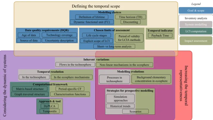
Many temporal considerations have been described in previous pub-lications, reports and standards to develop the general LCA framework (ISO14040, 2006;ISO14044, 2006;Joint Research Center, 2010) and its dynamic counterpart. For instance,Sohn et al. (2020)classified 56 DLCA studies by their technological domains and types of assessed dy-namism. In this section, the considerations arefirst regrouped by their purposes. A Venn diagram inFig. 2presents this organisation of tempo-ral considerations where gold, purple and red rounded rectangles re-spectively highlight the purposes of defining the temporal scope, considering the dynamic of systems and increasing the temporal repre-sentativeness. 10 classes of temporal considerations are also presented with rectangles of different colours and linked to the phases of the LCA framework where they most commonly appear. InFig. 2, the inter-pretation phase is excluded because the identified temporal consider-ations arefirst accounted for in the three mentioned phases and can then be used to analyse the results.
The level of relevance, conceptual development and operationalisation for the temporal considerations ofFig. 2are qualitatively assessed with scores ranging from A (highest) to C (lowest) (detailed inTable 2) to eval-uate the state-of-the-art shown inTable 3. A more detailed analysis, includ-ing examples, is provided in the followinclud-ing subsections to clarify the
3 1 3 2 7 3 12 7 10 13 18 22 34 31 46 80 81 90 127 132 167 207 185
qualitative appraisal ofTable 3. Possible temporal feedback between the LCI and LCIA are not assessed, although they may influence LCA results (Weidema et al., 2018).
3.1. Phase of goal and scope definition
In the goal and scope definition, temporal considerations can be in-troduced by the modelling assumptions, data quality requirements (DQRs) and model limitations. They mostly offer insights on the tempo-ral scope in which LCA studies are representative and useful. This tem-poral scope also provides an indication of when the dynamic of systems should be considered.
3.1.1. Modelling choices
3.1.1.1. Definition of lifetime. The lifetime of systems or products, which frames the use phase of the life cycle, is probably the most common temporal consideration in LCA studies (Anand and Amor, 2017; AzariJafari et al., 2016;Fitzpatrick, 2016;Helin et al., 2013;Mehmeti et al., 2016). This temporal scope, which is relative to the overall life cycle, has often been used to ensure a fairer comparison (Joint Research Center, 2010;Jolliet et al., 2010). However, more comprehen-sive temporal information on the full life cycle, which is not mandatory in international LCA standards (ISO14040, 2006;ISO14044, 2006), would be necessary to explicitly frame the full temporal scope over which elementaryflows and impacts might occur. For example, a house can be used for a lifetime of 50 years (Hoxha et al., 2016;
Standardisation, 2009), but this temporal scope does not include the phase of forest growth, which supplies wood for the fabrication of the building's components (Breton et al., 2018;Fouquet et al., 2015) or for advanced biofuels (Albers et al., 2019a).
3.1.1.2. Dynamic functional units. Some practitioners have suggested that the temporal scope should always be provided with the definition of questions (Finnveden et al., 2009;Huang et al., 2012;Ling-Chin et al., 2016) and functional units (FUs) (Inyim et al., 2016;Santero et al., 2011). The concept of dynamic FUs has been proposed (Kim et al., 2017), which could consider the evolution and comparability of prod-ucts and would explicitly define the period of validity for a LCA study when the behaviour of consumers and markets have changed signi fi-cantly. For example, the rapid evolution of technologies for mobile phones has changed their functionalities and demand thus modifying their global production volumes.
3.1.2. Data quality requirements (DQR)
3.1.2.1. Age of data. Some metadata of datasets, which should be defined in the DQR (ISO14044, 2006;Joint Research Center, 2010), informs on their age and minimum length of time for data collection. Potential temporal discrepancies between used datasets and the targeted temporal scope of a modelled system can thus be partially evaluated. Such information also provides some insights on the temporal scope of a system model when it represents human activities (Bessou et al., 2013;Yuan et al., 2015). For example, the description of solar energy
Table 1
List of proposed terms defining key temporal considerations in the LCA framework. The list is in alphabetical order so all terms from this glossary are underlined to highlight the links. Words in brackets are synonyms from the literature.
Term Definition
Dynamic LCA (DLCA) LCA studies where relevant dynamic of systems and/or temporal differentiation offlows are explicitly defined and considered.
Dynamic LCI (DLCI) Life cycle inventory (LCI) that is calculated from supply and value chains where dynamic of systems or temporal differentiation is considered, resulting in temporal distributions to describe elementaryflows.
Dynamic LCIA (DLCIA) Characterisation models of environmental mechanisms that account for the dynamic of ecosphere systems and can therefore use temporal information of DLCIs. The chosen temporal differentiation (e.g. day, season, and year) can depend on the impact categories. Both case specific and calendar-based characterisation models can be used, depending on the chosen indicators.
Dynamic of systems System modelling that considers inherent variations, periods of occurrence or evolution within the temporal scope of models' components. Such a dynamic modelling can be applied to both technosphere systems (for LCI) and ecosphere systems (for LCIA).
Evolution Changes of process, structure or state models' components (e.g. technology replacement, pollutant concentration in a compartment of the environment).
Inherent variations Variations offlows in the models' components (e.g. cycles of solar energy production, growth rates of vegetation, seasonal functional traits, biogeochemical and biophysical dynamics). The discontinuities offlow rates are also part of such changes.
Models' components Information structuring all models. At the technosphere level, components are elementaryflows, product flows and processes. At the ecosphere level, components of LCIA models differ between impact categories. For example, components for freshwater ecotoxicity can be environmental fate, ecosystem exposure and ecotoxicological effects (Fantke et al., 2018).
Period of occurrence The moment when a model's component is starting, modified or finishing over time. (e.g. lifespan of a building, beginning of waste management, start of a life cycle) Period-specific
characterisation factor (CF)
CF for a given temporal scope or period of occurrence. It results from the dynamic of systems in the ecosphere and can be calendar-specific, relative to the length of the temporal scope, or defined by a TH. Period-specific CFs are modelled as constant over the chosen period.
Period of validity The period over which datasets, LCIs or LCIA methods are considered valid representations. This information should be calendar-based. [Time context (ILCD), time frame, range of time, period of time, time period, timespan, temporal boundary, time scale and time horizon]
Prospective modelling A prospective LCA addresses future life cycle impacts using different modelling strategies (e.g. scenario-based, technology development curves and agent- or activity-based models). The evolution of systems is thus defined and/or simulated using a list of explicit assumptions regarding the future. Prospective modelling can be applied to both the technosphere and ecosphere and is a subset of the dynamic of systems, which only concerns future forecasts.
Temporal considerations
Any aspects (i.e. information) described in relation to the time dimension or dynamic of systems in the LCA framework. This is the overarching term relating to all other terms of the glossary. [Time-aspect in ILCD documents]
Temporal differentiation
The action of distributing the information on a time scale related to the models' components. For example, elementaryflows could be described per day or year. Different processes representing yearly average are another example. [Temporal segmentation in ILCD]
Temporal resolution Describes the time granulometry when temporal differentiation is carried out. For instance, a monthly or daily resolution can be used to describe the flows in technosphere models. The same term can be used to describe a time step for period-specific CFs. [Time step]
Temporal representativeness
Qualitative or quantitative assessment of data, processes or LCIA methods in relation to how appropriate their informationfits with their temporal scope. [Time-related representativeness (ILCD), Time-related coverage (ISO14044)]
Temporal scope Defines any type of period that is considered in a LCA study (e.g. temporal considerations along a life cycle, service life of a product, data collection period).
Temporalisation Attribution of temporal properties to the models' components. (e.g. definition of temporal scopes)
installations from the 1990s would probably be relevant for LCA of solar energy before 2000. Nevertheless, using such periods of validity require expert opinion, thus limiting the usefulness for this kind of metadata. 3.1.2.2. Technology coverage. In some cases, the definition of technol-ogy coverage in the DQR of datasets can inform on the actual tempo-ral scope of the study (ISO14040, 2006; ISO14044, 2006; Joint Research Center, 2010) with the ensuing qualitative assessment of temporal representativeness. For example, ecoinvent (Wernet et al., 2016) usesfive levels of technology (i.e. new, modern, current, old and outdated) to describe transforming activities. Using datasets with new or modern technology levels should therefore be relevant for LCA studies on future products. However, this information is rel-ative to each sector, as the modern level could be representrel-ative for 10 years of technology evolution in an established sector, whereas fast-paced sectors like electronics may use modern technologies for only 1 year before switching to new options.
3.1.2.3. Source of data. The choice of data sources and the qualitative as-sessment of their overall representativeness provide an indirect assess-ment of the temporal scope for modelled systems and LCA studies (Rebitzer et al., 2004). For example, when data are sourced from scien-tific journals, date of publication is the primary indication for its period of validity. More precise temporal information is also often provided in case studies for systems with longer lifetimes or in DLCA studies like
(Heeren et al., 2013;Pahri et al., 2015;Sohn et al., 2017a;Vuarnoz et al., 2018). The use of up-to-date LCA databases can bring a false sense of security on the temporal scope and representativeness of the data for recent products or systems. Indeed, database updates do not al-ways follow the changes in market shares or evolution of technology be-cause of the lack of new data.
Nevertheless, different temporal metadata is given for most datasets. For instance, ecoinvent guidelines (Wernet et al., 2016) require the def-inition of the date of generation, the date of review and the period of va-lidity with a start date and end date for any dataset. These temporal considerations fulfil most of the requirements from ISO 14044 (2006) except for the definition of the averaging period of dataset inputs. The ILCD handbook (2010) has set further requirements defining temporal properties: the expiring year of datasets and the duration of the life cycle, which respectively relates to the period of validity for LCI datasets and the temporal scope of elementaryflows for a dataset. This metadata is available in most datasets of the ELCD (Recchioni et al., 2013). Many of these temporal metadata are more relevant to assess the temporal scopes of studies than the choice of a database and its version, but the place (e.g. in dataset descriptions) and the different definition under which they can be found hinder their use in most LCA studies. 3.1.2.4. Uncertainty description. The description of the uncertainty as-sociated withflows (e.g. in ecoinvent (Wernet et al., 2016)) is an-other indirect source of information to clarify the temporal scope
Increasing the temporal
representativeness
s
me
ts
ys
f
o
ci
ma
n
y
d
e
ht
g
ni
re
di
s
n
o
C
Defining the temporal scope
Definition of lifetime
Dynamic functional unit (FU) Discounting Time horizon (TH) Modelling choices
Age of data Technology coverage Source of data Uncertainty description
Data quality requirements (DQR)
Life cycle stages
Short- vs long-term analysis Explicit scope of LCI
Period of validity for LCIA methods Chosen limits of assessment
Payback Time Temporal indicator
Matrix-based structure Graph traversal structure
Period-specific CF Characterisation functions Computational framework
DyPLCA Temporalis Approach & tool
Processes in technosphere
Background elementary concentration in ecosphere Modelling evolutions
Flows in the technosphere Non-linear mechanisms in the ecosphere Inherent variations
Historical trends Simulation approaches
Scenarios Strategies for prospective modelling In the technosphere In the ecosphere mechanisms
Temporal resolution
Goal & scope Inventory analysis System modelling LCI computation
Impact assessment
Legend
Fig. 2. Venn diagram of temporal considerations in relation to their purposes (grey rectangles), the phases of the LCA methodology (coloured rectangles) and 10 classes (Bold titles). Existing connections are presented by arrows.
Table 2
Meaning of different scores for the qualitative assessment of temporal considerations in LCA.
Ranking categories A B C
Relevance Demonstrated at least in some LCA studies Expected by authors of this article Unknown Conceptual
development
A standard method is accepted by the LCA community
At least one method for consideration has been proposed
Theory or concepts have been explained Operationalisation Available in the data of most LCA studies when
relevant
and period of validity. Indeed, the temporal correlation indicator provides a quantitative assessment of the discrepancy between the time when the data was acquired and the intended temporal scope for the dataset (Weidema et al., 2012). For example, a productflow with a temporal correlation indicator of 3 means that its value has been gathered between 6 and 9 years before or after the targeted temporal scope of the dataset. With the current definition of the temporal correlation indicator, the precision of this temporal infor-mation is rather low (i.e.N3-year period) and is widely missing in LCA databases and studies, limiting its applicability.
3.1.3. Chosen limits of assessment
The definition of limitations in the stage of goal and scope definition is probably the step where temporal scopes are defined with higher pre-cision and clarity in LCA studies, even more in recent DLCA studies. While this is useful, typical LCA reports mainly offer qualitative de fini-tions, which are not sufficiently transparent to describe the considered period in assessed life cycles.
3.1.3.1. Considered stages of the life cycle. LCA studies can limit the tempo-ral scope of their analysed systems and LCIs by considering only a part of the life cycle. Setting the end-of-life outside the boundaries is an exam-ple of such a limited temporal scope. The ISO 14044 (2006) allows this limitation, but only if they do not significantly change the overall con-clusions of a study because such phases are not linked to significant im-pacts. Most of the LCA reports clearly state the excluded life cycle stages, but they often provide an imprecise description for the limitation of the temporal scope. Moreover, the specification of the considered stages of a life cycle will not explicitly state the temporal scope in which elemen-taryflows are considered (e.g. 2 years) nor offer a calendar-based period of occurrence (e.g. from January 2019 to December 2020).
3.1.3.2. Temporal scope of life cycle inventories. More specific and precise descriptions of temporal scopes for LCI have been provided in recent sci-entific publications that focus on some temporal considerations (i.e. DLCA). For example, relative temporal scopes have been used to define the periods of LCIs for many studies on different products, for example considering the lifetime of wood-based products and buildings between 50 and 100 years (Fouquet et al., 2015;Levasseur et al., 2010) including tree growth period over 70 and 150 years (Levasseur et al., 2013; Pinsonnault et al., 2014), lifetime of marine photovoltaic of 20–30 years (Ling-Chin et al., 2016) and zinc fertiliser over 20 years crop rotation (Lebailly et al., 2014). In these cases, the LCIs are enclosed within a quantified period of time that can be relevant for some impact categories, but they lack any reference to a calendar year or period. Sev-eral DLCAs studies defined calendar-based temporal scopes, but discus-sions on the potential usefulness of this contextual information could be further enriched. Some were based on reference calendar years of build-ing materials (Collinge et al., 2013b), hourly energy demand in build-ings (Vuarnoz et al., 2018), as well as seasonal and annual variations in crop rotations (Caffrey and Veal, 2013). Other studies were based on calendar-specific periods detailing domestic hot water production (Beloin-Saint-Pierre et al., 2017), future biomass production (Menten et al., 2015), the lifetime of buildings (Roux et al., 2016a;Roux et al., 2016b), the energy use in hourly, daily and monthly temporal resolu-tions (Collinge et al., 2018;Karl et al., 2019), or for introducing back-time horizon (Tiruta-Barna et al., 2016).
3.1.3.3. Short- vs long-term analysis. Several publications describe the temporal scopes of technosphere models (Dandres et al., 2012; Menten et al., 2015) or LCI (Finnveden et al., 2009; Morais and Delerue-Matos, 2010; Pettersen and Hertwich, 2008; Roder and Thornley, 2016) with adjectives such as short-, medium- or long-term. These qualitative and relative attributes thus inform the considered
Table 3
List of temporal considerations in the LCA framework. Rankings for relevance, conceptual development and operationalisation are provided for each consideration on a scale from A to C with their colour code (seeTable 2). The colour for the three columns of purpose is based on the code ofFig. 2. The numbers for the rows are the text's subsections.
Sections Subsection Temporal considerations Defining
temporal scope Considering dynamics of systems Increasing temporal representativeness Relevance Conceptual development Operationalisation 3.1 Phase of goal and scope definition
3.1.1 Modelling choices Definition of lifetime X A A A
Dynamic FU X A B B
3.1.2 Data quality requirements (DQRs) Age of data X A A B Technology coverage X A B B Source of data X A C A Uncertainty description X A B B 3.1.3 Limits of assessment
Considered life cycle stages X A A A
Temporal scope of LCI X A B B
Short- vs long-term X A C B
3.2 Phase of inventory analysis: System modelling
3.2.1 Inherent variations Flows in technosphere X A B B
3.2.2 Temporal resolution In technosphere X B B B
3.2.3 Modelling evolution Processes in technosphere X A B B
3.2.4 Prospective modelling Simulation approaches X X B B B Historical trends X X A B B Use of scenarios X X A B B 3.3 Phase of inventory analysis: LCI computation 3.3.1 Framework Matrix-based X A B B Graph traversal X A B B
3.3.2 Approach and tool DyPLCA X A B B
Temporalis X A B B
3.4 Phase of impact assessment
3.4.1Modelling choices Time Horizons X A A A
Discounting X C B C
3.4.2 Limits of assessment Period of validity X B B B
Short- vs Long-term X A C B
3.4.3 Temporal indicator Payback time X B B B
3.4.4 Inherent variations Non-linear mechanisms X X B B C
3.4.5 Temporal resolution Ecosphere mechanisms X B C C
3.4.6 Modelling evolution Background concentration X X B B C
3.4.7 Prospective modelling Scenarios X X B B B
3.4.8 Computational framework Period-specific CFs X X B B B
Characterisation functions X X C C C
3.4.9 Approach and tool DyPLCA X A B B
periods, but are vague. This lack of a precise temporal definition can be partly explained by the lack of consensus on how temporal scopes should be defined.
3.2. Phase of inventory analysis: system modelling
In the system-modelling step of the LCI phase, temporal consider-ations are found in the descriptions of the system inherent variconsider-ations and evolution. They define the dynamics of systems and can improve the temporal representativeness of models for technosphere activities (i.e. network of processes). Although considering system evolution and inherent variations in both the foreground and the background data is still not a common practice, its importance has long been ac-knowledged in ISO 14040 (2006), stating that“all significant system var-iations in time should be considered to get representative results”.
Strategies to consider inherent variations and evolution have been proposed by different authors, mainly for energy (Amor et al., 2014; Zaimes et al., 2015), transport (Tessum et al., 2012), agriculture (Fernandez-Mena et al., 2016;Yang and Suh, 2015) and waste manage-ment (Bakas et al., 2015). For example, the energy share of electricity production in a country varies throughout days, weeks, months and sea-sons (Beloin-Saint-Pierre et al., 2019;Vuarnoz and Jusselme, 2018). LCA case studies have shown that inherent temporal variations of produc-tion can have significant effects on results, mainly when consumption of these products is not constant over time.
3.2.1. Inherent variations withflow differentiation
Inherent variations can be modelled with temporal differentiation of flows or dynamic modelling. For instance, electricity production (Messagie et al., 2014;Vuarnoz and Jusselme, 2018;Walker et al., 2015) and its use in buildings (Collinge et al., 2013b;Collinge et al., 2018;Karl et al., 2019;Roux et al., 2016b;Roux et al., 2017;Vuarnoz et al., 2018;Walzberg et al., 2019a), cloud computing (Maurice et al., 2014) and wastewater treatment (de Faria et al., 2015) have all been modelled with such approaches. In different ways, all these approaches convertflows into temporal distributions, thus supplementing temporal properties to the core data of the model components in the LCA frame-work. The applicability of such data in other LCA studies is often limited because the temporal information is valid only for the temporal scope of a given case study. A way to address this limitation is to use a reference “time 0” in the temporal distribution as a period of occurrence relating to a starting period of a process (Beloin-Saint-Pierre et al., 2014; Tiruta-Barna et al., 2016). This“time mark” creates process-relative de-scriptions, which can be reused in any period of a life cycle or even for different life cycles.Tiruta-Barna et al. (2016)andPigné et al. (2020) provided process-relative temporal distribution archetypes for ecoinvent v3.2, applicable to foreground and background datasets. As underlined byBeloin-Saint-Pierre et al. (2014), the additional efforts needed to provide temporal information for all theflows of LCA data-bases are still significant and the prioritisation of data-gathering re-mains important.
3.2.2. Temporal resolution
The level of temporal resolution to models the dynamics of systems depends on the sector and the modelling approach. For instance, hourly resolutions have been chosen for electricity production and consump-tion (Amor et al., 2014) or the transportation sector (Tessum et al., 2012). For assessing long-term emissions, for instance from waste treat-ment, a temporal resolution of centuries is more appropriate (Bakas et al., 2015). Some authors have proposed a temporal differentiation based on archetypes. For example, archetypal weather days (Risch et al., 2018) have been developed to contrast the relative importance of episodic wet weather versus continuous dry-weather loads. So far, studies about the consequences for choosing different temporal resolu-tions to describe theflows are limited. Indeed, only two examples are found in the building sector where a monthly resolution is deemed
sufficient to consider most of the temporal variability ( Beloin-Saint-Pierre et al., 2019;Karl et al., 2019).
3.2.3. Modelling evolutions with process differentiation
The basic strategy to describe evolution is to differentiate processes when a system is considered to change substantially over time. The key challenge here is to identifying when changes are significant enough without expert opinion on the modelled product. A simple ap-plication can be performed, if calendar-based periods of validity are consistently provided for all datasets in LCA databases; they could then be changed automatically when they are no longer valid represen-tations over the full life cycle of any system. Such metadata is, however, required only in the (discontinued) ELCD database (see subsection 0) and, currently cannot be easily integrated in LCA software.
Collet et al. (2011)proposed an approach to tackle this problem and identify where temporal differentiation of processes during sys-tem modelling is needed. Their general idea is to recognise when the combined emission and impact dynamics justify the additional effort for temporal differentiation. Moreover, the selective introduction of the time dimension in background processes has been studied by Pinsonnault et al. (2014)and more recently byPigné et al. (2020). The authors have shown that the temporal variations of a selection of background processes and the entire ecoinvent database can sig-nificantly affect climate change impacts for processes in some sec-tors (e.g. transport and building).
3.2.4. Prospective modelling
Modelling future evolution of systems is another common example of temporal considerations that is often performed under the umbrella of DLCA studies. Indeed, many DLCA studies have explored different prospective models for a range of products like: photovoltaic panels (Pehnt, 2006;Zhai and Williams, 2010), buildings (Collinge et al., 2013a;Frijia et al., 2012;Scheuer et al., 2003;Sohn et al., 2017a;Sohn et al., 2017b;Su et al., 2017), bioethanol (Pawelzik et al., 2013), passen-ger vehicles (Bauer et al., 2015;Miotti et al., 2017;Simons and Bauer, 2015), metals (Stasinopoulos et al., 2012) or ammonia (Mendivil et al., 2006). Any temporal assumptions made to define future evolution are thus considered for system modelling and LCI calculations. While major advances have been reached to offer explicit descriptions of as-sumptions made for temporal considerations in DLCA, e.g. (Collinge et al., 2013b;Herfray and Peuportier, 2012; Menten et al., 2015; Pehnt, 2006;Roux et al., 2016b), they are currently not the standard. Prospective modelling assumptions can be grouped within three cate-gories that have fundamental differences on how they justify their forecasting.
3.2.4.1. Simulation approaches. Economic models, such as partial equilib-rium models (PEM) or general equilibequilib-rium models (GEM), are fre-quently used in, but not limited to, consequential LCA modelling to simulate potential future evolution to assess direct and indirect conse-quences of decisions (e.g. climate policies) on large scale systems. Nevertheless, the current focus of using these models to assess conse-quences of changes in LCA studies should not hide their potential to offer possible development paths in prospective assessments. PEM gen-erally focuses on one particular economic sector with a higher level of detail (i.e. technology rich), while GEM covers the whole economy with a lower level of detail (typically 30–50 economic sectors). For in-stance, PEMs have been used to model the energy sector in France (Albers et al., 2019c;Menten et al., 2015), or biogas production in Luxembourg (Marvuglia et al., 2013) and GEMs have been used to eval-uate the consequences of different energy scenarios on the whole econ-omy in Europe (Dandres et al., 2011). PEMs have also been coupled with GEMs to model the consequences of energy policy scenarios in an inte-grated manner (Igos et al., 2015) and they have been used in combina-tion with dynamic models of biogenic and soil organic carbon for a similar purpose (Albers et al., 2020;Albers et al., 2019b).
The lack of consideration for human behaviour in PEM or GEM has recently been pointed out as a potential issue for the validity of the pro-spective models (Marvuglia et al., 2015). The use of agent- or activity-based models have therefore been proposed as alternatives to carry out prospective assessments; both in the foreground and in the back-ground systems. Such models have mostly been used in consequential LCAs relating with transport policies (Querini and Benetto, 2015), re-gional market penetration of electric vehicles (Noori and Tatari, 2016), switch grass-based bioenergy systems (Miller et al., 2013), smart build-ings (Walzberg et al., 2019b) or raw materials criticality (Knoeri et al., 2013), but could be used to predict future trends. The differences be-tween the use of such simulation approaches in DLCA or consequential LCA studies have been discussed recently bySohn et al. (2020).
3.2.4.2. Forecasting based on historic trends. Some data sources (e.g. sta-tistics on energy production) describe historic trends from which fore-casting is made by extrapolation, assuming paradigm shifts will not occur. For instance, regression analysis was used to assess the evolution of energy systems (Pehnt, 2003a;Pehnt, 2003b;Pehnt, 2006;Yang and Chen, 2014) and the construction sector (Sandberg and Brattebø, 2012). The main strength of this approach is its simplicity and the potential to assess the observed level of variability of historic trends. It can thus pro-vide averaged future trends and the expected variability (uncertainty). The main weakness, on the other hand, is the implicit assumption that historic trends are representative of the future, which is not always the case, particularly for emerging systems and technologies.
3.2.4.3. Using scenarios to explore potential futures. Scenario-based modelling has been used in many sectors like waste management (Hellweg et al., 2005), water consumption (Pfister et al., 2011), bioenergy (Choi et al., 2012;Daly et al., 2015;Dandres et al., 2012; Earles et al., 2013;Igos et al., 2014;Menten et al., 2015), renewable elec-tricity (Hertwich et al., 2015;Pehnt, 2006;Viebahn et al., 2011), trans-port (Cheah and IEEE, 2009;Garcia et al., 2015;Pehnt, 2003a;Pehnt, 2003b), chemicals (Alvarez-Gaitan et al., 2014) and buildings (Roux et al., 2016b). A general idea behind modelling scenarios is that explor-ing many potential futures may be simpler to justify than offerexplor-ing pre-dictions on what the future will look like for a system as complex as human activities. For instance,Pesonen et al. (2000)defined that the scenarios describe possible future situations based on assumptions about the future and include developments from the present to the fu-ture. The authors distinguished between“what-if” and “cornerstone” scenarios (Pesonen et al., 2000), depending on the need to consider short- or long-term planning.“What-if” scenarios are often based on thefield-specific expertise of LCA practitioners. Cornerstone sce-narios explore many options with very different assumptions on the future to identify potential development paths. Another category is legally bound scenarios that explore future paths under the restric-tion of regularestric-tions.
3.3. Phase of inventory analysis: LCI computation
The computation of LCI transforms the information of a technosphere model into a set of elementaryflows whose quantities are in relation to the FU of the assessed systems. The computation tradi-tionally aggregates allflows of the same type over the entire life cycle. 3.3.1. Computational framework
3.3.1.1. Matrix-based computation with process differentiation. The con-ventional matrix-based computational approach can be used to calcu-late DLCIs, but with larger technosphere and ecosphere matrixes (Heijungs and Suh, 2002).Collinge et al. (2012, 2013b)used this ap-proach on foreground processes to calculate the DLCI for each year of a building's life cycle. They concluded, similarly toHeijungs and Suh (2002), that the implementation brings significant challenges in data
management when background databases are used. The challenges of this approach are twofold. Firstly, the temporal description of a system needs to be re-informed when the periods of assessment differ (e.g. 1980–2000 vs 2005–2025), if considered impacts are calendar-based. Secondly, the amount of data and the computational efforts depend on the required temporal precision (e.g. day vs. year) to de-scribing allflows.
3.3.1.2. Graph traversal structure. The Enhanced Structure Path Analysis (ESPA) approach (Beloin-Saint-Pierre et al., 2014) is one type of graph-based computational framework that convolves process-relative temporal distributions (seeSection 3.2.1) to propagate the tem-poral descriptions offlows. The general concept behind the ESPA frame-work (Beloin-Saint-Pierre et al., 2014;Maier et al., 2017) relates to one strategy of graph traversal algorithms (i.e. breadth-first), but other op-tions have been explored. The depth-first search strategy ( Tiruta-Barna et al., 2016) recommends a different traversal of supply chains, which is normally linked to lower memory requirements. The best-first search strategy (Cardellini et al., 2018) is another option that prop-agates the temporal information by prioritising the temporal distribu-tion with higher contribudistribu-tions to impacts. All these opdistribu-tions use process-relative temporal distributions, thus profiting from their reus-ability and the potential for higher temporal precision.
3.3.2. Approaches and tools
Some commercial software tools use matrix-based computation (e.g. Simapro, Umberto) and could thus work with the process differen-tiation framework for the calculation of temporally differentiated LCI. To our knowledge, this option has not been implemented comprehensively in DLCA studies because LCA databases do not offer temporal details. The ESPA method has also not been developed into a computational tool and its implementation has been limited to one simplified case study (Beloin-Saint-Pierre et al., 2017). Nevertheless, two options cur-rently exist for full DLCI computations and are introduced in the follow-ing sub-sections.
3.3.2.1. DyPLCA. DyPLCA has been implemented as a web tool (available athttp://dyplca.univ-lehavre.fr/), originally presented byTiruta-Barna et al. (2016), which uses the depth-first graph search strategy. The main parameters that balance accuracy vs. computation time in this tool are the temporal resolution of function integrals and the back time span. Common values for both are respectively 1 day and −50 years (i.e. 50 years before the period of occurrence for the FU). The computational intensity of the DLCI calculation has thus been re-solved by a trade-off between accuracy and cut-offs. The process-relative temporal distributions can have different levels of detail to de-scribe theflows in the system models. For instance, they can be detailed for foreground processes, as presented inShimako et al. (2018), and can be rather generic for the background datasets.
DyPLCA currently works with a temporal differentiated ecoinvent v3.2 (Pigné et al., 2020), providing generic temporal descriptions to most background inventory processes. The DLCI results can be further used with static or DLCIA methods, as shown in studies on bioenergy production from microalgae (Shimako et al., 2016) and on grape pro-duction (Shimako et al., 2017).
3.3.2.2. Temporalis. Temporalis (Cardellini et al., 2018) is a free and open source package of the Brightway2 LCA tool (Mutel, 2017), using the best-first search strategy. The tool is fully compatible with many existing commercial LCA databases, but temporal de-scriptions of datasets are currently not provided. Temporalis does not require afixed and continuous temporal resolution over any sys-tem models to provide DLCI or results for the impact assessment. Nevertheless, a DLCIA method for GWP based on the IPCC methodology (2013), is included. A simple case study for the tempo-ral consideration of biogenic carbonflows was carried out with the
method ofCherubini et al. (2011, 2012). It has shown that the LCI computation can be resolved on a regular laptop within a short time. Nevertheless, further developments still need to be completed before most LCA practitioners can use the tool easily.
3.4. Phase of life cycle impact assessment
In the LCIA phase, temporal considerations affect many aspects that are linked to all phases of the LCA framework. For instance, the selection of a TH and changes of environmental mechanisms (i.e. impact path-ways) over time are key modelling choices to characterise impacts in a DLCA framework.
3.4.1. Modelling choices
LCIA is a complex task that requires many assumptions (e.g. the fu-ture state of the environment) and choices, which sometimes limit the validity of results to a specific temporal scope and introduce bias in the results. One of the most explicit and commonly used temporal con-siderations in LCIA methods is the TH, restricting the impact assessment to a specific period. Discounting is another modelling choices that can affect LCA results in similar ways to TH with links to its potential subjec-tivity (Lueddeckens et al., 2020).
3.4.1.1. Time horizon. The choice between afinite or infinite TH is a com-mon type of temporal consideration that sums the environmental ef-fects over a selected temporal scope (e.g. the 100-year TH for the GWP indicator). The consideration of different THs is used, for instance, by the ReCiPe method (Huijbregts et al., 2016), which builds on three cultural perspectives, proposed byHofstetter et al. (2000). These per-spectives are associated with different sets of calculation assumptions, including CFs with different THs for each impact category. For example, the“hierachist” perspective retains a 100-year TH for GWP and other categories, while“individualist” and “egalitarian” perspectives respec-tively use THs of 20 and 1000 years. Furthermore, very long THs are sug-gested for some impact categories such as for climate change (i.e. 1000 years) and ionising radiation (i.e. 100,000 years). The ILCD hand-book (2011) and the SimaPro Database Manual (PRé, 2016) provide ad-ditional insights into the use of THs in different LCIA methods, but there is not yet any standard on how to deal with long-term impacts and re-lated uncertainties within all categories. For instance, the 5thIPCC assessment report (2014)removed the 500-year TH due to high uncer-tainties associated with the assumption of constant background concentrations.
To date, the choice of a TH remains a topic of discussion within the LCA community (Dyckhoff and Kasah, 2014;Reap et al., 2008b) where three critical aspects are challenging the use offixed and finite THs in LCIA methods:
• The first aspect is the inconsistency between the temporal boundaries of the studied systems and the TH of the LCIA methods (Benoist, 2009; Levasseur et al., 2010;Rosenbaum et al., 2015;Yang and Chen, 2014). Indeed, it could be understood that effects from elementaryflows be-yond the chosen TH should not be considered. However, the effects are ultimately modelled over an invariable temporal scope, even if they occur at different periods during a life cycle (e.g. 100 years). This use of THs may thus lead to misrepresentations of impacts and their period of occurrence (Hellweg and Frischknecht, 2004), for in-stance, misleading decision-making concerning temporary storage and emission delays (Brandao and Levasseur, 2011;Jørgensen et al., 2015). This issue can be particularly significant for intermitting emis-sions like pesticides, where arbitrary cut-offs of emisemis-sions after pesti-cide application should influence how each emission contributes to related impacts of human toxicity (Fantke and Jolliet, 2016) and ecotoxicity (Peña et al., 2019).
• The second aspect refers to the time integration of substances with highly variable environmental effects over their lifetime in the
ecosphere (e.g. aging effects reducing bioavailability of metals (Owsianiak et al., 2015) or transformation of persistent chemicals in the environment (Holmquist et al., 2020)), which can significantly bias the conclusions of LCA studies (Arodudu et al., 2017;Lebailly et al., 2014). In the case of GWP, the weight of forcers with very short atmospheric residence time decreases with an increasing TH (Levasseur et al., 2016;O'Hare et al., 2009), while a shorter TH in-creases the importance of short-lived gases. For example, methane (CH4), whose atmospheric lifetime is about 12.4 years, goes from a factor of 84 CO2-eq for the 20-year TH to a factor of 28 CO2-eq for 100-year TH (Myhre et al., 2013). For further examples on this subject, Levasseur et al. (2016)presented various approaches that have been proposed for TH definition. For toxic substances,Huijbregts et al. (2001)demonstrated that TH variations can change impacts by up to 6.5 orders of magnitude for metal toxicity. In this case, the high de-pendency between CFs and the chosen TH is due to long residence times (i.e. persistence) in fate models, which increase metal run-offs and leaching potential to global marine and soil compartments. • The third aspect relates to the temporal cut-offs that come with the
selection of afixed and finite THs, which can be ethically questioned in the context of intergenerational equity (Hellweg et al., 2003a). In-deed, these cut-offs raise concerns on the subjectivity of choosing a specific TH to highlight preferences between short- and long-term im-pact considerations (Lueddeckens et al., 2020). For instance, the 100-year TH in GWP is the most used and recommended option, but this preference is not justified by scientific facts (Reap et al., 2008b; Shine, 2009;Vogtländer et al., 2014) and is implicitly subjective for decision-making (Brandao and Levasseur, 2011;Fearnside, 2002). This 100-year TH is particularly important when temporary/perma-nent carbon storage or the delayed emissions from biogenic and fossil sources are evaluated or incentivised (Guest and Stromman, 2014; Levasseur et al., 2012a). Moreover, emissions that are delayed after the 100-year scope are then considered to be permanently avoided (BSI, 2011;Joint Research Center, 2011).
A“simple” solution to remove such time preferences and value choices has been recommended by setting infinite THs in all cases. For instance, some LCIA methods (e.g. EDIP2003 (Hauschild et al., 2006), IMPACT 2002+ (Jolliet et al., 2003), ReCiPe 2016 (Huijbregts et al., 2016)) use infinite or indefinite THs as a standard for stratospheric ozone depletion, human toxicity and ecotoxicity. In the case of the land use impact category, THs are generally not ex-plicitly stated in current characterisation models (see e.g.Huijbregts et al. (2016)for biodiversity impacts orMüller-Wenk and Brandão (2010)for climate change). Even if the theoretical frameworks for land use impact assessment discusses changed (Beames et al., 2015) or permanent impacts and therefore the need for defining a TH (Canals et al., 2007;Koellner et al., 2013), permanent impacts are currently not considered in available characterisation models. Current models implicitly correspond to the choice of an infinite TH where impacts of each land use intervention is being integrated over time until the effect factor reaches 0, i.e. until the variations of soil quality after the land use intervention regenerates back to a ref-erence soil quality. Regeneration time then plays a significant role in the effective integration period and in the definition of CFs. 3.4.1.2. Discounting. This concept was discussed to value time in LCIA (Hellweg et al., 2003a;Pigné et al., 2020;Yuan and Dornfeld, 2009; Zhai et al., 2011) and to deal with the uncertainties associated with time preferences and future emissions. The setting offinite THs is an im-plicit form of discounting for long-term impacts, using a zero discount rate over the TH, and an infinite discount rate beyond the TH. Discounting offers a trade-off between giving a higher value to present or future impacts. A more detailed discussion on this subject is provided byLueddeckens et al. (2020).
3.4.2. Chosen limits of assessment
The periods of validity for chosen LCIA methods and discussions on the short- or long-term nature of impacts are two types of tempo-ral considerations that can inform on the tempotempo-ral scope of a LCA study, whether this selection is voluntarily made by the practitioner or not.
3.4.2.1. Period of validity for LCIA methods. Stating the period of validity (e.g. 2000 to 2010) or version for chosen LCIA methods in LCA studies is not common practice, but it can provide insights on the expected tem-poral scope (Bessou et al., 2011;Hauschild et al., 2013;Ling-Chin et al., 2016;Weidema et al., 2012). The choice of THs can also suggest an im-plicit definition of the considered period of validity. In an ideal world, the temporal scope of obtained LCIs and chosen LCIA methods should befitted to each other. Such a correspondence is desirable if CFs vary significantly over time, but it is currently difficult to implement in the available databases and software tools.
3.4.2.2. Short- vs long-term analysis. Much like it has been said in the def-inition of the goal & scope (Section 3.1.3), the adjectives of short- and long-term have been used to describe the temporal scope of LCIA methods (Arodudu et al., 2017;Chowdhury et al., 2017;Reap et al., 2008b). This lack of a precise temporal definition when stating short-, medium- and long-term can be partly explained by the differences in time scales of life cycles and environmental impacts for different sys-tems. Furthermore, a commonly accepted standard does not yet exist to deal with long-term impacts and related uncertainties within all cat-egories. For instance, the 5th IPCC assessment report (Myhre et al., 2013) removed the previously published 500-year TH due to the high uncertainties associated with the assumption of constant background concentrations.
3.4.3. Temporal indicator
3.4.3.1. Payback time. Payback times have been created to provide a temporal scope that informs on temporality of impacts. The basic idea is to calculate the necessary period to compensate for the “cra-dle-to-gate” impacts of any system. It has been mostly used to eval-uate the time it takes to produce an amount of electricity that is equivalent to the primary energy use from the manufacturing of photovoltaic installations (Espinosa et al., 2012; Fthenakis and Alsema, 2006;Knapp and Jester, 2001), but it can be applied to en-ergy use in many types of product (Elshout et al., 2015) or could also give payback time for other impact categories.
3.4.4. Inherent variations
In conventional LCIA methods, CFs are determined with average or marginal approaches that model changes in the impact according to a change in the inventory (Frischknecht and Jolliet, 2016; Hauschild and Huijbregts, 2015). With this average approach, the environmental disturbances from different activities are aggregated, historically referred to as“snapshots” of a studied system (Bright et al., 2011; Heijungs and Suh, 2002; Klöpffer, 2014; Levasseur et al., 2016;Owens, 1997b;Vigon et al., 1993). For example, most existing models for characterising toxic impacts (Rosenbaum et al., 2008) assume constant environmental conditions for the assessment of health impacts. With this approach, inherent variations of the eco-sphere are not considered.
3.4.4.1. Non-linear mechanisms in the ecosphere. The marginal approach addresses an impact resulting from a small change to a given back-ground concentration. The impact is therefore positioned in relation to the current environmental state. For example, studies of human health impacts from exposure tofine particulate matter (PM2.5), where indoor, outdoor, urban and rural locations have shown significant differences in PM2.5background levels (Fantke et al., 2017). A non-linear
exposure-response model thus accounts for these differences in PM2.5levels, reflecting a slope for low concentrations that are substantially higher than for high concentrations (Fantke et al., 2019).
Impact assessment models are representations of complex environ-mental mechanisms that depend on a long list of parameters, such as the lifetime of substances in the environment and the sensitivities of ecosystems over different temporal scopes (Lenzen et al., 2004). In many LCIA methods, CFs are defined from generic parameters values in stationary conditions (e.g. intervention quantity, baseline for target substances, and profiles of the soil composition) or for a given TH. Sub-sequently, impacts are assumed linearly proportional to the inventoried emissions, which enable the scaling of impacts to any functional unit. In reality, the involved environmental mechanisms are dynamic and often highly complex (Arbault et al., 2014). They depend on the physical, chemical and biological phenomena and non-linear interaction occur-ring in nature and are consequences of the elementaryflows generated by human activities.
Time-dependent characterisation has been performed in some cases by modelling the dynamics for one or more of the three factors influencing an impact (i.e. environmental fate, exposure, and ef-fects), thus creating a type of DLCIA methods. Effect data are typically not easily linked to temporal properties, allowing for temporal con-siderations in effect modelling (e.g. dose response for human effects or concentration response for ecological effects). Hence, time-dependent characterisation is usually only facilitated by considering the dynamics of systems in the fate and exposure factors of an impact pathway, which is usually enabled by models of the underlying mass balance for a given impact pathway. This has been implemented, for example, in toxicity-related impacts (Lebailly et al., 2014), where the system dynamics of the environmental fate factor are either solved via numerical integration (Shimako et al., 2017), or via matrix de-composition (Fantke et al., 2013).
3.4.5. Temporal resolution
3.4.5.1. Specific temporal resolution for each elementary flow. The tempo-ral considerations within LCIA models may follow specific frequencies (e.g. yearly changes), as well as temporal-inherent features deriving from dynamic biogeochemical processes. The frequency can be differen-tiated, for instance, as responding to episodic (e.g. initial land clearing), cyclical (e.g. seasonal water and pesticide use), stochastic (e.g. 1 in 20 years' waste discharge), or continual (e.g.fisheries yields) variations in the studied system (Lenzen et al., 2004). Cyclical or seasonal varia-tions concerning sunlight, temperature and precipitation on the calen-dar year (e.g. winter vs summer time) are other examples of temporal considerations that could be relevant for impact categories like aquatic eutrophication (Udo de Haes et al., 2002), water scarcity (Boulay et al., 2015), human toxicity (Manneh et al., 2012) and photochemical oxi-dant formation (Shah and Ries, 2009). Such frequencies therefore high-light relevant temporal resolutions for the temporal differentiation of elementaryflows in databases and DLCIs. Temporal inherent features may vary with hourly, daily, monthly or yearly constraints depending on temporal patterns or modelling time steps of the characterisation models (Collet, 2012;Owens, 1997b).
The temporal scope of impact assessment itself may be aligned with the dynamics of governing biogeochemical processes to more accu-rately represent certain fate dynamics. For instance,Liao et al. (2015) found that common seeding-to-harvest assessment periods in agricul-tural LCAs do not correspond to the actual dynamics of fertilising sub-stances, some of which contribute to eutrophication during the next crop rotation. The same concerns agricultural pesticides, where the time between the application and crop harvest drives related residues leading to human exposure (Fantke et al., 2011). Such fate dynamics can still be analysed and parameterised tofit steady-state models and associated impact pathways, such as human toxicity (Fantke et al., 2012;Fantke et al., 2013).
3.4.6. Modelling evolutions
3.4.6.1. Considering variations for concentration substances and the state of the environment. Elementaryflows may have varying levels of effect, de-pending on the timing of emissions (i.e. period of occurrence) and the state of the environment (i.e. varying substance concentrations). Tem-poral considerations of environmental mechanisms in LCA studies are challenging because the current state of practice rarely allows to ac-count for the periods of emission occurrences that are related to a product's life cycle (Finkbeiner et al., 2014;Hellweg and Frischknecht, 2004;Jørgensen et al., 2014;Kendall et al., 2009;Levasseur et al., 2010;Reap et al., 2008b). In fact, LCIflows are typically given as simple values that are considered to be a representation of steady or pulsed flows from and to the environment by most LCIA models. For instance, impacts characterisation methods often use an effect factor for a given concentration of pollutants in the background environment (Finnveden et al., 2009;Hauschild, 2005). Thus, the same amount and type of elementaryflows (i.e. equivalent LCIs) can generate different levels of impacts because they have been emitted at different periods of occurrence (e.g. 2016 or 2017), with varyingflows (i.e. inherent var-iations) and geographies, requiring both temporal and spatial differen-tiation. In this case, calendar specifications may be relevant to assess and compare the evolution of impacts and/or background concentra-tions over time (e.g. 1990 Kyoto Protocol and the 1750 IPCC reference years for climate change). The inherent variations in the state of the en-vironment can also affect the CFs. For example, temporary changes in the carbon cycle from land use (Vazquez-Rowe et al., 2014) and related changes in the albedo of the land surface are two dynamic aspects that can bring variations in environmental impacts (Bright et al., 2012). Such variations are currently difficult to assess since they are not linked to “standard” elementary flows, which are always the source of impacts in the usual LCA framework.
3.4.7. Strategies for prospective modelling
As is the case for technosphere models, it is, in principle, possible to forecast the environmental responses of the ecosphere to elementary emissions with the use of scenarios.
3.4.7.1. Scenarios. An alternative form of temporal considerations in LCIA is increasingly performed on scenario-driven case studies. It has been applied to water use impacts by means of scenario-bound CFs, where each scenario represents a different prospective TH (Núñez et al., 2015). It is a step towards considering the temporal variability of envi-ronmental indicators, as most LCIA methods make the implicit assump-tion that the environment and its properties will not evolve over the studied life cycle. Another common example is the case of metal leaching in ground that has been forecasted with different scenarios (Huijbregts et al., 2001;Pettersen and Hertwich, 2008).
3.4.8. Computational framework
Recently, some DLCIA methods have been developed with different computational frameworks. These approaches are key to understand the links between DLCIs and DLCIA methods, while offering potential pathways for future developments.
3.4.8.1. Period-specific characterisation factors. In the last decade, LCA re-searchers have developed DLCIA methods addressing time dependent impacts as a function of time, yet they are mainly restricted to GWP and toxicity indicators. These DLCIA methods consider the periods of occurrence for emissions by providing different period-specific CFs to assess their impacts. For example, CFs can be calculated for each year over a chosen time horizon or for the month of January 2020. These CFs thus bring consistency between the temporal scopes of DLCI and impacts (Levasseur et al., 2010). Different LCA scholars found that the results based on such DLCIA methods provide useful examples for decision-making, among others, on: “the intensity, extend and
frequency of the impacts” (Lebailly et al., 2014), the sensitivity of the results to various TH choices (Levasseur et al., 2012b), and the optimi-sation options from scenario-bound simulations (Shimako et al., 2017). The DLCIA method developed by Levasseur et al. (Levasseur et al., 2010) is currently one of the most recognised and sophisticated approaches, featuring period-specific CFs. In addition, calendar-specifications can be relevant to assess and compare the evolution of impacts and/or background concentrations over time (e.g. 1990 Kyoto Protocol and the 1750 IPCC reference years for climate change). 3.4.8.2. Time-dependent characterisation functions. Recent works (Shimako et al., 2017;Shimako et al., 2018;Shimako et al., 2016) have proposed to come back to the origins of impact simulation tools and adapt them by adding temporal information in the LCIA phase. The idea is to consider the opportunities of using DLCIs as inputs for DLCIA models. Such a DLCIA model has been proposed to assess toxicity im-pacts (human and ecotoxicity) byShimako et al. (2017)and has been applied in a full DLCA study. The model reintroduces the time dimen-sion for fate modelling of substances in the environment, providing the temporal distributions of substances in different environmental compartments. The physical parameters for the calculation of fate, ex-posure and effect factors were taken from the USEtox model. This method doesn't propose period-specific CFs, but directly calculates the impacts by coupling the impact model with all the available information in DLCIs.
The definition of ecotoxicity according to time also allows to evalu-ating the intensity of the impact for different periods of occurrence, which supports the identification of critical periods for potential im-pacts. The cumulated toxicity then represents the total damage gener-ated over a TH. When compared with conventional USEtox results, obtained in steady state conditions, the DLCA results are systematically lower, but toxicity tends towards the conventional results for an infinite TH. Non-persistent substances (generally organic) generate almost all their hazard potential during their periods of emission and disappear more or less rapidly due to the degradation or transfer to sink compart-ments (removal). In contrast, persistent substances accumulate in envi-ronmental compartments during the emission periods and their toxicity potentials remain high after the emissions stop, potentially affecting many human generations.
3.4.9. Approach and tools
As was explained inSection 3.3.2, some examples of using com-bined DLCI and DLCIA methods have been published recently for DyPLCA (Shimako et al., 2017;Shimako et al., 2016) and Temporalis (Cardellini et al., 2018) respectively for the toxicity and climate change categories. Still, this type of combination is rare and can only be done for few impact assessment methods with period-specific characterisation factors or time-dependent characterisation functions. Further developments are definitely required here to allow for a comprehensive consideration of the dynamics of impacts in future DLCA studies.
4. Proposed development pathways
It is rather straightforward to define key temporal considerations within the DLCA framework when the challenges of data availability and management are overlooked. Indeed, the general goal can be summarised by a desire to reach the highest level of temporal represen-tativeness and to provide useful information for analysis, when consid-ering the dynamic of systems in all of the model components. It would then seem relevant to:
• Clearly define calendar-based temporal scopes for all flows of a DLCI to outline the periods of elementaryflow occurrences that justify the choice for DLCIA methods with specific temporal scopes or THs. This temporal information would also set a clear temporal frame of