Selection of borehole temperature depth profiles for regional climate reconstructions

(1)

HAL Id: hal-00298170

https://hal.archives-ouvertes.fr/hal-00298170

Submitted on 19 Jan 2007

HAL is a multi-disciplinary open access

archive for the deposit and dissemination of sci-entific research documents, whether they are pub-lished or not. The documents may come from teaching and research institutions in France or abroad, or from public or private research centers.

L’archive ouverte pluridisciplinaire HAL, est destinée au dépôt et à la diffusion de documents scientifiques de niveau recherche, publiés ou non, émanant des établissements d’enseignement et de recherche français ou étrangers, des laboratoires publics ou privés.

Selection of borehole temperature depth profiles for

regional climate reconstructions

C. Chouinard, J.-C. Mareschal

To cite this version:

C. Chouinard, J.-C. Mareschal. Selection of borehole temperature depth profiles for regional climate reconstructions. Climate of the Past Discussions, European Geosciences Union (EGU), 2007, 3 (1), pp.121-163. �hal-00298170�

(2)

CPD

3, 121–163, 2007 Borehole selection C. Chouinard and J.-C. Mareschal Title Page Abstract Introduction Conclusions References Tables Figures ◭ ◮ ◭ ◮ Back Close Full Screen / Esc

Printer-friendly Version Interactive Discussion

EGU Clim. Past Discuss., 3, 121–163, 2007

www.clim-past-discuss.net/3/121/2007/ © Author(s) 2007. This work is licensed under a Creative Commons License.

Climate of the Past Discussions

Climate of the Past Discussions is the access reviewed discussion forum of Climate of the Past

Selection of borehole temperature depth

profiles for regional climate

reconstructions

C. Chouinard and J.-C. Mareschal

GEOTOP-UQAM-McGill, Centre de Recherche en G éochimie et en G éodynamique Universit é du Qu ébec à Montr éal, Canada

Received: 21 December 2006 – Accepted: 8 January 2007 – Published: 19 January 2007 Correspondence to: J.-C. Mareschal (jcm@olympus.geotop.uqam.ca)

(3)

CPD

EGU

Abstract

Borehole temperature depth profiles are commonly used to infer time variations in the ground surface temperature on centennial time scales. We compare different proce-dures to obtain a regional ground surface temperature history (GSTH) from an ensem-ble of borehole temperature depth profiles. We address in particular the question of

5

selecting profiles that are not contaminated by non climatic surface perturbations and we compare the joint inversion of all the profiles with the average of individual inver-sions. We show that the resolution and the stability of the inversion of selected profiles are much improved over those for a complete data set. When profiles have been se-lected, the average GSTH of individual inversions and the GSTH of the joint inversion

10

are almost identical. This is not observed when the entire data set is inverted: the average of individual inversions is different from the joint inversion. We also show that the joint inversion of very noisy data sets does not improve the resolution but, on the contrary, causes strong instabilities in the inversion. When the profiles that are affected by noise can not be eliminated, averaging of the individual inversions yields the most

15

stable result, but with very poor resolution.

1 Introduction

In recent years, borehole temperature data have been used to provide additional ev-idence for recent climatic changes in several parts of the world (e.g. Cermak,1971; Vasseur et al.,1983;Lachenbruch and Marshall,1986;Nielsen and Beck,1989;

Bel-20

trami et al., 1992; Wang, 1992; Bodri and Cermak, 1997; Pollack et al., 1996). In-deed, transient surface temperature perturbations propagate downward and, although attenuated, are recorded in the Earth′s subsurface as perturbations of a steady state temperature regime.

Because surface temperature oscillations are damped over a length scale δ (skin

25

depth) which depends on their frequencyω and on thermal diffusivity κ (δ= q

(4)

CPD

EGU the earth acts as a filter and the record of the ground surface temperature history

(GSTH) is blurred. Because of the low thermal diffusivity of rocks (_≈10−6m2s−1), the short period oscillations, such as the diurnal or annual cycles, have skin depth ranging from a few centimetres to a couple of meters. Variations of ground surface temperature of the last 200–300 years are recorded in the first 200 m, whereas the effect of the

post-5

glacial warming is observed down to 2500 m. The interpretation of temperature profiles in terms of the GSTH presents all the characteristics of ill-posed geophysical inversion problems: their solution is not unique and it is unstable (e.g.Jackson,1972;Tikhonov and Arsenin,1977;Menke,1989;Parker,1994).

The first application of inversion techniques to infer the GSTH from borehole

temper-10

ature profile was the study byVasseur et al.(1983). In the last fifteen years, several papers have addressed the problem of inversion of borehole temperature data and different methods have been proposed to invert the GSTH from one or several temper-ature profiles. Many other papers deal “empirically” with practical considerations.

The interpretation of borehole temperature profiles is based on the one dimensional

15

heat equation; it assumes that a uniform boundary condition is applied on a plane sur-face and that physical properties only depend on depth. Although corrections can be applied to correct heat flow for the effect of topography (Blackwell et al., 1980), this is rarely done in climate studies because the amplitude of the climatic signals is often smaller than the uncertainty on these corrections. Other variations in surface boundary

20

condition can affect the temperature measured at depth and need to be accounted for: proximity to lakes or large rivers, recent forest fires, changes in vegetation cover, defor-estation. Other perturbations include refraction by lateral changes in thermal conduc-tivity, water circulation in the borehole, etc. These effects need to be well documented since they produce distortions of the temperature profiles similar to those produced by

25

climate change and they might overshadow any real climatic signal in a GSTH. Until recently, borehole temperature depth profiles were not logged to infer past climates, but for heat flow measurements. For heat flow studies, corrections are often small and can be avoided when boreholes are deep and the surface effects become negligible.

(5)

CPD

EGU But for climate studies, the signal is recorded in the shallow part of the profile which is

most affected by “noise”.

It had been hoped that the problem of “noise” could be alleviated through regional GSTH studies, performed by inverting several borehole temperature profiles within a given region (Beltrami and Mareschal, 1992; Pollack et al.,1996). Such studies

as-5

sume that variations of air surface temperature trends and thus of ground surface temperatures remain correlated over distances_{≈500 km (}Hansen and Lebedeff,1987; Jones et al., 1999). Two methods can be used to determine a regional GSTH: all the borehole temperature profiles are inverted simultaneously to obtain the common GSTH, or each profile is inverted separately and the individual GSTHs are averaged.

10

If noise is random and uncorrelated, the simultaneous inversion of a given data-set, either local or regional, should theoretically yield a GSTH with a better signal to noise ratio than an average of individual inversions. This assumes that the noise is uncorre-lated and that there is no systematic bias in the perturbations of the temperature profile. This latter condition is unlikely to be met for practical reasons: for instance, boreholes

15

located on the shore of a lake can be (and are) logged, but boreholes in the middle of a lake never are. Some authors (Lewis,1998) have thus argued that the error associated to GSTH will systematically be biased towards a warming of the ground surface. The argument is that in most cases, human and/or natural effects on the energy balance at the ground surface will cause a gain of energy by the ground (clear-cutting of forested

20

areas, pollution effects on vegetation cover, forest fires, etc.). Previous studies with poorly documented site conditions retained all the boreholes and might have overesti-mated the warming trend (Beltrami et al.,1992;Beltrami and Mareschal,1992).

When the conditions at the sites are well documented, one could eliminate the tem-perature profiles that are perturbed by surface conditions. In general, very few

bore-25

holes meet strict criteria, and the majority of the logged boreholes in a region are rejected. For example, in two recent studies only 15 and 50% of the logged bore-holes within the study areas were retained (Guillou-Frottier et al.,1998;Gosselin and Mareschal,2003).

(6)

CPD

EGU The correlation of individual inversions of temperature profiles is often weak whether

they come from the same region (Gosselin and Mareschal,2003) or cover a wide part of the Earth surface (Harris and Chapman,2001). Consequently, the GSTH averaging all the individual inversions has very poor resolution (Pollack et al.,1998). It was hoped that the simultaneous inversion of profiles from a region that have recorded the same

5

GSTH would improve resolution because the signal in the GSTH should be correlated and the noise is not (Beltrami and Mareschal, 1992, 1995; Clauser and Mareschal, 1995;Pollack et al.,1996). In practice, this did not turn out to be true (Huang et al., 2000;Gosselin and Mareschal,2003). There are several reasons that joint inversion did not do much to improve the results.

10

1. The number of temperature profiles remains small and insufficient to produce a significant improvement in the signal to noise ratio which is∝√N.

2. The assumption that the GSTHs are identical is almost never verified. One would not expect it to hold when the data cover a very wide region of the Earth. Even at the regional scale, visual inspection of the reduced temperature profiles reveals

15

that they have not recorded the same GSTH. Thus, the joint inversion of real data seldom improves signal/noise ratio; sometimes it decreases this ratio.

3. Even when the GSTHs are identical at all sites, the records will be consistent only if the thermal diffusivity at each site is well determined. The danger of adjusting physical properties is that the GSTHs may appear well correlated when they are

20

not.

4. The resolution is limited by the profile with the highest noise level which deter-mines how much regularization is required (Beltrami et al.,1997).

5. Beltrami et al. (1997) have emphasized the need to combine profiles with com-parable vertical depth in order to avoid bias. The minimum depth sampled varies

25

(7)

ex-CPD

EGU tremely noisy and are often discarded. This is an important bias because

temper-ature perturbations are largest near the surface.

Different authors have calculated the GSTH (local or regional) from the raw or the “reduced” temperature depth profiles. The reduced temperature profile is obtained by removing from the data a reference temperature profile, obtained by upward

contin-5

uation of the lowermost part of the profile, assumed to be near steady state. This preprocessing of data allows to infer warming or cooling by visual inspection of these reduced profiles. But it may also be useful to improve the results of the inversions using the singular value decomposition algorithm to determine regional GSTH.

So far, there is no consensus among researchers on the best procedure to obtain

10

a regional GSTH (simultaneous inversion vs. average of individual inversions, selec-tion of borehole temperature profiles unaffected by non-climatic perturbaselec-tions vs. “in-discriminate” use of all the borehole temperature profiles, reduced vs raw tempera-ture profiles). No systematic studies were conducted because there were not enough measurements in a given region to make statistically relevant comparisons. During

15

the past 20 years, the GEOTOP-IPGP research team has logged 338 boreholes at more than 100 different sites across south-central and south-eastern Canada (Fig.1). Because these sites are distributed in three main regions, northern Manitoba and Saskatchewan, north-western Ontario, and eastern Ontario and Quebec, these bore-hole temperature data are appropriate to conduct regional studies, and the number of

20

data in each region is sufficient to compare results from the different procedures.

2 Theoretical framework

2.1 General formulation – the direct problem

Usually, the data consist of a few temperature profiles, thermal conductivity, and heat production measurements. Because the temperature profiles are sparse and the

bore-25

(8)

CPD

EGU in physical properties, and in the boundary conditions. These assumptions are not

al-ways satisfied either because the surface boundary condition can vary (effect of lakes, vegetation cover, topography, etc.) or because physical properties vary horizontally and there may be refraction. This is likely to be the case with mining exploration bore-holes that target very local mineralized bodies. In general, however, there is not enough

5

information on the 3-D conductivity variations and insufficient data to warrant a three dimensional model.

For a layered earth, the steady-state temperature profile can be written as:

Tez = Tref+qrefR(z) − M(z) (1) R(z) = Zz 0 d z′ λ(z′₎ 10 M(z) = Zz 0 d z′ λ(z′₎ Zz′ 0 d z”H(z”)

whereλ is the thermal conductivity, H is the heat generation, z is depth, positive down-ward. The heat flowqrefis taken positive upward. If a temperature perturbationT0(t) is

applied uniformly on the surfacez=0, the temperature in a homogeneous half space is given by (Carslaw and Jaeger,1959):

15 T_t(z, t) = z 2√πκ Zt 0 T0(t′) (_{t − t}′₎3/2 × exp −z2 4κ(t − t′₎ ! d t′ (2)

where the thermal diffusivityκ is assumed constant.

For a jump ∆T in surface temperature at time t before present, the temperature perturbation is given by:

T (z) = ∆T × erfc z

2√κt (3)

20

(9)

CPD

EGU temperature perturbation is given by:

T (z) = ∆T (1 + z 2 2κt)× erfc z 2√κt + z 2√κt × exp z2 4κt ! (4)

For a constant change in surface heat flux ∆q starting at time t before present, the temperature perturbation is (Carslaw and Jaeger,1959):

T (z) = 2∆q λ ( κt π) 1/2_{× exp}−z 2 4κt − z 2 × erfc z 2√κt ! (5) 5

and, in particular, the change in surface temperature is given by: T (z = 0) = 2∆q

λ ( κt

π)

1/2 ₍₆₎

Figure 2shows the temperature profiles for three different surface boundary condi-tions leading the same present surface temperature. As one would expect, warming is more rapid after a jump in surface temperature than after a jump in surface heat

10

flow. This is well known, but the point is that the reconstructed history depends on the boundary condition, which is poorly understood. For instance, using a heat flow boundary condition might lead to underestimating the time when the change in surface temperature conditions occurred.

It is possible to account for variations in thermal diffusivity with depth. Formal

so-15

lutions for the transient temperature in a layered half space are “easily” obtained with the Laplace transform (e.g.Carslaw and Jaeger,1959). The “Born approximation” to the general solution of the heat equation for continuously varying physical properties with depth is given in Shen and Beck (1991). Because thermal diffusivity variations are usually small, their effect on the transient temperature profile is a second order

20

perturbation that can safely be neglected in view of all the other sources of error, pro-vided that the average diffusivity is well determined. This does not hold true for the effect of conductivity variations on the steady state temperature profile which must be accounted for.

(10)

CPD

EGU 2.2 The inverse problem

For borehole temperature data, the inverse problem consists of determining, from the temperature-depth profile, the reference surface temperature and heat flow, and the ground surface temperature history. Determining the reference heat flow requires knowledge of the thermal conductivity variations, usually measured on core samples.

5

Alternatively, the thermal conductivity structure can be introduced as free model pa-rameters through the thermal resistance vs. depth Eq. (1), but in this case the inverse problem becomes non-linear.

Generally, the inverse problem can be expressed as an integral equation:

T (z) = Z0

−∞

∆_{T (t}′₎_{K (z, t}′₎_{d t}′ ₍₇₎

10

where the kernelK (z, t’) is given in Eq. (2). It turns out that this type of integral equa-tion always describes an ill-posed problem. If T(z) is known approximately, there is no solution to the inverse problem. Furthermore, an approximate solution is useless because the inverse operator is not continuous. The physical meaning of this instability is easy to understand. We can always add to the solution ∆T (t) a periodic function

15

N sin(ωt). Regardless how large N, the effect on the temperature profile T (z) can be made arbitrarily small by increasing the frequencyω. In other words, the difference between the exact and the approximate surface temperatures could be arbitrarily large at almost any time. This is paradoxical, but we do take advantage of this property because we are mainly concerned with long period trends. In inverting temperature

20

depth profiles, we can thus safely neglect the daily or the annual cycles although their amplitudes are at least ten times larger than those of the long term trends that we are trying to detect.

(11)

CPD

EGU 2.3 The inverse problem discretized

Because the temperature variations of short duration are filtered out of the temperature profile, any parametrization that allows to reproduce the gross features of the surface temperature history could be used. Many different parameterizations have been pro-posed for the GSTH: a discontinuous function corresponding to the mean surface

tem-5

perature duringK time intervals ∆_k (k=1, ....N), a continuous function varying linearly withinK intervals ∆k, a Fourier series, etc.

We shall assume that the GSTH is approximated by a discontinuous function cor-responding to the mean surface temperature duringK intervals of duration ∆_k (where the ∆_k can be adjusted to the resolution decreasing with time).

10

For a single temperature profile, the temperature Θj measured at depth zj can be written as:

Θ

j =AjlXl (8)

where Θ_j is the measured temperature at depthzj corrected for the heat production between the surface and that depth,X_l is a vector containing the unknowns_{T0,q0,T1,

15

...,T_K_{}, and A}_jl is a matrix containing 1 in the first column and the thermal resistances to depthzj,R(zj) in the second column. In columns 3 toK +2 the elements Aj,k+2 are obtained by calculating the differences between error functions at timest_k andt_k−1for depthz_j: A_j,k+2= erfc zj 2pκt_k ! − erfc zj 2pκt_k−1 ! (9) 20

whereκ is the thermal diffusivity. The other parameterizations mentioned above would yield a system of equations with the same structure.

Because the meteorological trends appear correlated over distances of ≈500 km (Jones et al.,1986;Hansen and Lebedeff,1987), boreholes from different sites in the same region may have recorded identical GSTH. If this is indeed the case, it is possible

(12)

CPD

EGU to derive this common GSTH from simultaneous inversion of all the temperature profiles

that have recorded seemingly consistent climatic signals. ForI boreholes, the unknown parameters are theI surface temperatures and heat flow values and the K parameters of the ground temperature history. The data are all the temperature measurements from all the boreholes. IfNi is the number of temperature measurements at borehole

5

i, the matrix has N1+N2+...+NI rows and K +2×I columns. The first N1 elements of

the first column equal 1 and all the others equal 0; the following N₂ elements in the second column are 1 and all the other elements are 0, and so on. The following I columns contain the thermal resistances to depthz_j in boreholei. Finally, the K last rows contain the differences between error functions at times t_k and t_k−1 for every

10

depth and every borehole. The resulting equations can be written as (Clauser and Mareschal,1995):      θ(1) θ(2) ... θ(I)      =      1 0 ... 0 R(1) 0 ... 0 A(1) 0 1 ... 0 0 R(2)... 0 A(2) ... ... ... ... ... ... ... ... ... 0 0 ... 1 0 0 ... R(I) A(I)      ×                  T₀(1) T₀(2) ... T₀(I) q₀(1) q₀(2) ... q₀(I) T                  (10)

where θ(i) denote the vectors of temperature data for borehole i and R(i) denote the vectors containing thermal resistance to each depth in boreholei; the elements of the

15

matrix A(i)are the differences between error functions at timet_kandt_k−1for each depth of boreholei. Thermal diffusivity is usually assumed constant within each borehole but varies between boreholes. The unknown parameters are theI reference surface temperaturesT₀(i ), theI reference heat flows q(₀i ), and theK parameters of the common

(13)

CPD

EGU ground surface temperature history contained in the vector T.

2.3.1 Regularization by singular value decomposition

The system of N linear equations defined by Eqs. (8) and (10) must be solved for the_{M=K +2×I unknown parameters. In general, the system is both underdetermined} and overdetermined, and it is unstable. If the system of equations Ax=b is

mixed-5

determined, a generalized solution can be obtained by the singular value decomposi-tion (SVD) (Lanczos,1961;Press et al., 1992). It involves the decomposition of the (N×M) matrix A as follows:

A = UΛVT (11)

where superscript T denotes the transpose of a matrix. The matrix U is an (N×N)

10

orthonormal matrix (i.e. a rotation matrix) in data space,V is an (M×M) orthonormal matrix in parameter space, and Λ is an (N×M) diagonal matrix; the only nonzero el-ements are theL “singular values” λ_l on the diagonal, L≤min(N, M). The generalized solution is given by

x = V Λ−1UTb (12)

15

where the (M×N) matrix Λ−1 is a diagonal matrix with the L elements 1/λl on the diagonal (for λ_l _{6 =0) completed with zeros. The instability of the inversion results} from the existence of very small singular values. In practice, this problem can be alleviated either by retaining only the_{P ≤L singular values larger than a given “cutoff”} or by damping the reciprocals of the smaller singular values. The damping is done by

20

replacing the reciprocals of the smaller singular valuesλ_l by 1

λl →

λ_l

λ2_l +_ǫ2 (13)

where ǫ will be referred to as damping or regularization parameter. The impact of noise can be reduced by selecting a higher value ǫ, which, however, decreases the

(14)

CPD

EGU resolution (Beltrami et al.,1997). For borehole temperature data, the value ofǫ ranges

between 0.01 and 0.1. It is usually slightly higher than the singular value cutoff (_≈0.01). Both methods yield GSTH’s that are relatively close. Although there is no compelling argument to prefer one method over the other, damping usually gives smoother results than the sharp cutoff.

5

3 Description of the data

The borehole temperature profiles used in this study were obtained by researchers at GEOTOP and at the Institut de Physique du Globe de Paris (IPGP) over the past twenty years. The measurements were made for determining heat flow in the Canadian Shield and are described in a series of papers (Pinet et al.,1991;Mareschal et al.,2000,2005;

10

Perry et al.,2006).

This study separates in three regions all the borehole temperature depth profiles logged for heat flow determination in the Canadian Shield by the GEOTOP-IPGP team over the past 20 years (Fig. 1). In order to give the same weight to deep boreholes in the simultaneous inversion, all boreholes deeper than 550 m were truncated to that

15

depth. Also, since shallow boreholes are very difficult to reduce with accuracy and to invert, they could affect the simultaneous inversions. Therefore, all boreholes shallower than approximately 350 meters were automatically rejected.

The boreholes located in central Canada between the provinces of Saskatchewan and Manitoba were logged between 1993 and 1999. Table1shows the location of all

20

these boreholes with their depth and a remark explaining if it was retained for inversion or the reason why it was rejected.

The second region selected in this study covers a large part of north-western Ontario. Most of the boreholes in this region were logged between 2000 and 2005 and their locations, depths and remarks are shown in Table2.

25

The third region covers the eastern part of Ontario and the western part Quebec. The temperatures measurements were made for heat flow determination between 1987

(15)

CPD

EGU and 1993. The location, depth and remarks for each borehole are given in Table 3.

Because at that time the objective of the measurement was not the study of climate change, the surface conditions were not sufficiently documented to select boreholes suitable for inversion. Only, the shallowest boreholes have been eliminated from the study. Analysis of this data-set will allow to compare the trends in three different regions

5

when all the measured boreholes are retained for inversion.

For all profiles, temperature measurements are made at 10 m intervals using an electrical cable and a probe equipped with a thermistor. The precision of these mea-surements is of the order of 0.002 K and the overall accuracy is better than 0.02 K. The GEOTOP-IPGP research team is equipped with several cables ranging from 600 m to

10

2.3 km and with probes capable of measuring temperatures in the range between –15 to 50 degrees Celsius.

For each borehole, core samples were collected to measure their thermal conduc-tivity. Usually, the core is sampled every 80–100 m, and wherever important changes in lithology occur. Thermal conductivity is determined by the method of divided bars

15

(Misener and Beck,1960). Heat generation is also determined for the heat flow stud-ies. Heat generation is usually low in the Canadian Shield and has little effect on the shallow part of the temperature profiles, and it can be ignored except for very deep boreholes.

Each profile was carefully examined and when necessary erratic data points in the

20

shallow part of the profile were removed. These erratic values are caused by the probe not equilibrating with the groundwater or by water movement near the ground surface. A test was performed to verify that this removal does not affect the GSTH. A synthetic temperature depth profile was inverted using first the complete profile, then the same profile without the first 30 m, and finally the same profile without the first 60 m. The

25

results showed almost no difference in the GSTH between the complete and the profile truncated above 30 m, while the resolution of the recent past decreases for GSTH obtained from the profile truncated above 60 m. This test shows that the removal of one or two data points in the topmost 20 m of many boreholes does not strongly affect

(16)

CPD

EGU the recent part of the GSTH.

4 Results

4.1 Tests with synthetic data

The SVD method for simultaneous inversions has been thoroughly tested for regional GSTH by using multiple series of 84 synthetic temperature depth profiles containing a

5

ground surface temperature history signal of 600 years similar to those appearing in recent publications for central and eastern Canada (Guillou-Frottier et al.,1998; Gos-selin and Mareschal,2003;Beltrami and Mareschal,1992). Each synthetic tempera-ture depth profile had random noise added to it; this noise had approximately the same level we observe in measured data. We verified that varying some parameters of the

10

synthetics (noise level, sampling interval, total depth of the profile, reference gradient and surface temperature) does not affect the GSTH.

Most of the parameters mentioned above had little or no effect on the simultaneous inversions. However, we noticed instabilities when the average of all reference temper-atures had a value other than 0. Large oscillations appeared in the GSTH as well as

15

a jump in surface temperature at the beginning of the history. We carefully examined and interpreted the resolution matrices as showing a spill-over of the reference tem-peratures to the rest of the matrix when a large number of profiles were simultaneously inverted.

In order to prevent this “spill-over” of the reference temperatures into the solution,

20

it was simply removed by using the reduced temperature profiles (i.e. the difference between the observed and reference profiles). When properly reduced, a profile only shows the perturbations to the steady-state temperature in the borehole without any information on the reference temperature or gradient. Further tests with series of syn-thetic temperature depth profiles showed that GSTHs obtained from reduced profiles

25

(17)

CPD

EGU Although no problems were identified when using observed temperature profiles for

individual inversions or simultaneous inversions using a limited number of profiles, it is recommended to use reduced profiles when inverting simultaneously many profiles. 4.2 Study with real data: selection of profiles and interpretation

4.2.1 Manitoba-Saskatchewan

5

The first data set analyzed was from the Saskatchewan-Manitoba region (Fig. 1), con-sisting of 106 boreholes logged between 1993 and 1999. First, all boreholes shallower than approximately 200 m were eliminated. This was necessary because the reference gradient for such shallow profiles is too poorly constrained for the profiles to be reduced. Also these shallow profile do not provide the desired time window for this study.

An-10

other 3 boreholes (9903, 9904 and 9905) from the Kississing Lake site were removed from the dataset because the lake effect was so overwhelming that it overshadowed the signal of the other profiles. This limited to 73 the number of usable boreholes for the regional study in Saskatchewan-Manitoba. From these 73 boreholes, only 13 were considered affected by no other surface condition than a temporal change in the ground

15

surface temperatures. Table1lists all the boreholes in the region with their character-istics and the non-climatic effects that were noted. The reduced temperature profiles for the entire data set show a lot of variability and seem inconsistent; however, the 13 retained profiles are much more similar and consistent with each other. All the profiles are shown in Fig.3a. Since most of these profiles are affected by non-climatic factors,

20

the variability is considerable, although an overall warming trend is clearly visible and can also be inferred from the average GSTH. If only the 13 unaffected temperature depth profiles are plotted (Fig.3b), the variability decreases dramatically and not only the amplitude of the recent warming, but the onset of the little ice age (LIA) is also apparent. However it is also worth noting that the average of the reduced temperature

25

profiles of the entire and selected datasets are almost identical.

(18)

CPD

EGU in this study (i.e. 20 year time steps covering 600 years). Thermal conductivity and

diffusivity were assumed constant for all inversions in this paper and heat production values were not taken into consideration.

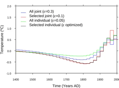
The 73 temperature depth profiles were inverted simultaneously with the same parametrization and a value for regularization parameter, ǫ=0.3. A larger

regular-5

ization parameter than for the individual inversions is necessary because the singular values are different and decrease more slowly than those of individual inversions. In or-der to obtain comparable information between individual and simultaneous inversions, one needs to use approximately the same number of singular values for both. Thus, the cut-off needs to be higher in simultaneous inversions than in individual inversions.

10

The result from the simultaneous inversion was then compared with a simultaneous inversion using only the 13 selected profiles and is shown in Fig.4.

One of the problems of most inversion techniques is the occurrence of instabilities due to the inversion. Actually, the main difficulty is the proper tradeoff between stability and resolution. In the case of SVD, the instability affects the larger singular values and

15

thus the recent past in the GSTH: It is seen as marked oscillation at 20–40 years before present. In this study, the inconsistencies between the records of various boreholes are causing these instabilities. It casts serious doubt that any conclusion concerning the very recent past can be derived from the simultaneous inversion of noisy records. In the data space, the corresponding eigen vectors sample mostly the shallow part of the

20

profile, which is noisiest, i.e. the most affected by non-climatic surface perturbations. To alleviate the instability problem and to gain perspective on the resolution of the simultaneous inversions, we calculated the averages of inversion for all the individual profiles from the complete and the selected data-sets. Each profile from the complete data-set of 73 profiles was inverted, using the same regularization parameter for all

25

the profiles (ǫ=0.05), but adapting the parametrization for the shallow profiles. These individual GSTHs were then averaged in order to obtain a regional GSTH. For the 13 selected profiles, each inversion was optimized by using the smallest regularization parameter possible while preserving the stability of the inversion. There is a major

(19)

CPD

EGU difference between the results obtained from the entire dataset and those from the

se-lected profiles. It concerns the LIA minimum (ca. 1820 AD), which is more pronounced in the selected profiles than with the entire dataset. There are two factors explaining that difference of amplitude. First, as mentioned above, the 13 selected profiles were inverted using unique optimized regularization parameters, meaning each individual

5

inversion was optimized for maximum signal to noise ratio. This optimization is im-possible to perform on the complete data-set (73 profiles) because the signal is often non-climatic, and the optimization would amplify the noise. Without even amplifying the noise, the many profiles (60 out of of 73) that recorded non-climatic effects will domi-nate the average and yield near zero temperature perturbation at the time of the LIA.

10

It is noteworthy that individual inversions are performed independently and that there is no constraint to fit a unique model, whereas a simultaneous inversion does have this constraint. In profiles severely affected by non-climatic perturbations, the climatic signal can be taken into consideration by the simultaneous inversion. So in the case of a simple average of individual inversions, the fact that all GSTHs have the same

15

weight means that random non-climatic perturbations will weight heavily on the overall average.

On the other hand, the average of individual inversions has the advantage of being more stable than a joint inversion. Since these instabilities are usually not correlated to the climatic signal, the average of several GSTH will ultimately cancel most of the

20

instabilities and yield a reasonable value in the interval 20–40 years before present (Fig.4).

4.2.2 Northwestern Ontario

The second data-set analyzed for this study was from Northwestern Ontario (Fig.1). It consists of 56 boreholes logged between 2000 and 2003. All boreholes shallower

25

than approximately 200 m were eliminated. All the profiles in the dataset are displayed on Fig.5a. Temperature depth profiles from two more sites were removed from the data-set because of the overwhelming effects they had on the inversions. The profiles

(20)

CPD

EGU (0306, 0307 and 0308) from the Junior Lake site where an important forest fire had

occurred a few years before measurements were eliminated. We also eliminated the profiles from Seagull (0112 and 0113) because of the overwhelming effect of water and gas rushing out of an over-pressured zone at depth. The perturbed Seagull profiles are easily identifiable on Fig.5a. Water was still rushing out of the borehole several weeks

5

after the drilling operations had stopped. The complete dataset of usable boreholes for northwestern Ontario contained 35 boreholes. From this set, 15 were considered unaffected by non-climatic perturbations. The description of the boreholes and the rea-sons for eliminating some profiles are listed in Table2. The resulting reduced profiles are shown on Fig.5b. The complete dataset includes some very noisy profiles. As in

10

central Canada, the selected profiles exhibit more consistent trends than the complete data set, but the average reduced profiles of both datasets are similar.

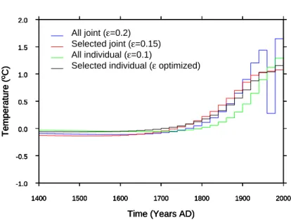
As for Manitoba-Saskatchewan, we obtained four different regional GSTHs by invert-ing jointly and by averaginvert-ing individual inversions of the complete and of the selected datasets (Fig.6).

15

The inversions were performed with the same temporal parametrization as for Manitoba-Saskatchewan (20 year time steps covering 600 years before present). How-ever, because the northwestern Ontario boreholes were generally noisier than those in Saskatchewan-Manitoba a higher value was selected for the regularization parameter of individual inversions (ǫ=0.1).

20

The regional GSTH using the complete dataset of 35 temperature depth profiles and the selected dataset of 15 profiles were inverted with a regularization parameterǫ=0.2 and 0.15 respectively. Despite the high noise level, the regularization parameter is smaller than the one used for Manitoba-Saskatchewan region mainly because there are less temperature depth profiles (and thus lower singular values) in the complete

25

data set than in Manitoba-Saskatchewan. On Fig.6, the GSTHs are reasonably similar until 100 years before present. But the GSTH for the complete dataset is very unstable in the most recent 100 years, showing a serious warming followed by a sudden 1.0 K drop over a 20 year interval and a 1.25 K jump in the last 20 year step. This clear

(21)

non-CPD

EGU climatic signal is most likely due to the sum of two factors: 1) an effect of the noisier

profiles measured in that region, and 2) the inversion instability.

The average of the individual inversions for the region confirms that this oscillation is due to the instability of the inversion. For the individual inversions, each profile contained in the complete dataset was inverted with a regularization parameterǫ=0.1;

5

the profiles contained in the selected dataset were all optimized using the best signal to noise ratio possible (smallest regularization parameter). The results are also plotted against the simultaneous inversions on Fig.6. This suggests that the large oscillation in the simultaneous inversion of the complete dataset is non-climatic, since none of the averages show such a jump.

10

The study of western Ontario has also shown that simultaneous inversion of all bore-holes in a given region regardless of the site conditions is likely to lead to an erroneous GSTH. A single very perturbed profile has the potential to cause major non-climatic shifts in the final GSTH. This happened with the accidental inclusion of the Seagull site (boreholes # 0112 and 0113) in the data set. The resulting GSTH was very much

15

affected, showing a full degree drop in temperatures with the minimum occurring at the exact time of the LIA minimum (1780 AD). This apparent LIA signal was due only to the inclusion of the Seagull site where the temperature profile was extremely perturbed by the gushing out of water and gas that persisted years after drilling. The GSTH without that site contains no LIA signal in western Ontario.

20

A comparison of the curves obtained by averaging individual inversions of both datasets shows similar GSTHs for the first 300 years and then some divergence in the recent most past, as was observed in the averages of Manitoba-Saskatchewan. As was the case in Manitoba-Saskatchewan, the presence of profiles perturbed by random non-climatic effects in the complete dataset tends to bring the average near

25

zero.

The obvious difference between the first two regions is the absence of any LIA signal from the western Ontario datasets. Regardless of noise level or depth, we could not see a LIA cooling period in the GSTH from any of the profiles and are confident that it

(22)

CPD

EGU is missing in that part of Canada.

4.2.3 Eastern Ontario and Quebec

The third dataset used for this study contains the oldest measurements taken by the GEOTOP-IPGP research team in Quebec and in eastern Ontario between 1987 and 1992 (Fig. 1). As mentioned before in this paper, these measurements were taken

5

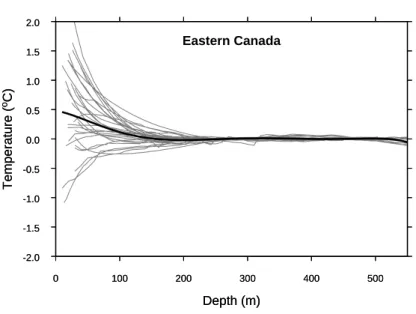
solely for heat flow studies and there is very little documentation on the actual mea-surement sites. Because of this lack of information, the analysis of the data from this region was done only on the complete dataset, as it was impossible to identify non-perturbed sites with certainty. Although a total of 137 boreholes had been measured, the complete dataset consists only of 28 usable boreholes because many of these

10

boreholes are too shallow and/or severely perturbed (Table3). The reduced profiles are displayed on Fig.7. Like in the other two regions, these profiles are quite inconsis-tent, but the average of all the reduced profiles is not very different from those obtained in the other regions. When we revisited some of these sites, we found out that they were affected by non-climatic perturbations. Some of these 28 boreholes would thus

15

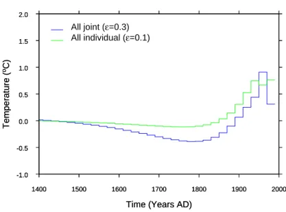
be rejected if we could apply the same strict criteria as in the other two regions. The 28 temperature depth profiles were all individually inverted using the same parametrization as for the other regions and ǫ=0.1. The regional GSTH for eastern Canada was performed by simultaneously inverting the complete dataset of 28 tem-perature depth profiles with a regularization parameter ǫ=0.3. As for the other two

20

regions, an average of individual inversions was also performed in order to compare the two methods as well as the effects of potential instabilities. Both curves are plotted in Fig.8. The difference in amplitude of the LIA minimum (1800 AD) between the joint inversion and the average is similar to that observed in central Canada and has the same explanation, the weight of the random non-climatic perturbations minimizing the

25

GSTH. Therefore, we think that the LIA signal detected in eastern Canada is real. For the recent past (past 60 years), there are differences between the two curves. The joint inversion yields a very unstable GSTH in the very recent past (recent most 60 years).

(23)

CPD

EGU This is another indication that the shallow section of some of the profiles is dominated

by noise (i.e. non climatic effects). The regional GSTH obtained from the average of individual inversions probably yields the best (i.e. most stable) GSTH for that period, as the instabilities are canceling out in the averaging process.

5 Discussion

5

The study was undertaken to compare different procedures to process and invert a regional GSTH from borehole temperature depth profiles, in particular: (1) Is it better to select boreholes that are not affected by non climatic perturbations, or does the noise from these perturbations cancel out? (2) Is it better to perform a joint inversion of all the temperature depth profiles than to average the results individual inversions? The most

10

important conclusion is that the results obtained by different procedures remain fairly consistent with each other, and the differences between methods are less than the error limits. Provided the inversions are carried out with sufficient care, similar trends will be inferred from all the procedures. This does not mean that they yield identical results. When choosing a particular procedure, we are faced with the standard problem

15

of the tradeoff between resolution and stability of the inversion.

– Whenever possible, i.e. when the sites are well documented, it is much better to

select temperature profiles that are not perturbed by non-climatic effects near the surface. Regardless of the method used (joint inversion or averaging of individual inversions), the GSTHs have higher resolution and are more stable than those of

20

the entire dataset.

– Because selected profiles are less noisy than all the profiles from a region and

the resolution is determined by the level of noise in the noisiest of the profiles, it is better to invert jointly selected profiles. In other words, the joint inversion of non selected profiles does not improve at all the resolution which is degraded by

25

(24)

CPD

EGU eigen vectors in data space that correspond to the large singular values sample

the shallow part of the profile that is most affected by the non-climatic perturba-tions. The resolution is improved by selecting profiles that are not affected by non-climatic signals.

– The average of all the GSTHs from a region has very poor resolution. The indi-5

vidual inversions of all the profiles from a region always yield GSTHs that are very inconsistent with each other. This supports the view that the non-climatic effects are more or less random, but these effects often overwhelm the climatic signal in the individual inversions.

– This study comforted us in the opinion that few good data always yield much better 10

results in terms of resolution and stability than many low quality data. Whenever possible, i.e. when there is a sufficient number of profiles that are well docu-mented, a selection of profiles should be made.

– When profiles are selected, individual inversions yield consistent results. If each

individual inversions is optimized, the resolution of the average of the individual

15

inversions is better than that of the joint inversion of the same profiles. The re-gional GSTH should be obtained both by averaging individual inversions and by joint inversion of the selected profiles.

– The comparison of GSTHs using complete and selected temperature depth

pro-files, show no systematic warming trend due to non-climatic perturbations. If there

20

were systematic warming effects on these perturbed profiles, these would be ap-parent in the different comparisons of GSTH techniques presented in this paper. However, contrary to the suggestion byLewis (1998), there does not seem to be any sign of bias in the data and no systematic warmer trend in the GSTH obtained from all the profiles measured in a region than in that obtained from selected

pro-25

(25)

CPD

EGU Determining the ground surface temperature history from borehole temperature

pro-files in south-central and southeastern Canada has been the object of many studies (Nielsen and Beck, 1989; Beltrami and Mareschal, 1991, 1992; Wang et al., 1994; Guillou-Frottier et al.,1998;Majorowicz et al., 1999;Gosselin and Mareschal,2003). Our results are consistent with previous results, but because different approaches were

5

used to process the data, our study clarifies the problems of resolution and robustness of the regional GSTH. Our results are consistent with each other but differ in resolution with some trends that are well marked only with some methods.

– Regardless of the method used, there seems to be a warming signal ranging

between 0.5 and 1.0 K over the past 500 years with some regions experiencing

10

different warming rates. The LIA signatures obtained in Manitoba-Saskatchewan and and in eastern Canada are consistent and appear almost synchronous (with very limited time resolution). This suggests that the LIA occurred simultaneously across the central and eastern parts of Canada.

– On the other hand, the LIA is not found in northwestern Ontario, which is lo-15

cated between these two regions. This point was also discussed byGosselin and Mareschal (2003). Although the Ontario profiles are in general noisier and shal-lower than those in Manitoba-Saskatchewan, we do not believe that this explains the absence of the LIA. Regardless of the depth or noise level of the profiles, none of the individual inversions shows the LIA cooling. Two boreholes (logged by the

20

Geological Survey of Canada in the early 1980s) located in northwestern Ontario but more than 500 km to the north of our study area do show a LIA signal. One possibility is that the LIA did not occur near Lake Superior because the the local climate is affected by the lake.

– All regional GSTHs performed with selected temperature depth profiles show ei-25

ther a decrease or a stabilization of the warming rate in the recent past (20–40 years ago) before the most recent warming. This is in agreement with meteoro-logical data from weather stations located in or near Central Canada, (as shown

(26)

CPD

EGU in Fig. 10 from Gosselin and Mareschal,2003). These mean annual surface air

temperature data, smoothed by averaging over an 11 year window, show a cooling trend from the 1940s to the 1970s. Despite the 20 year steps used in the regional GSTHs and the difference between surface air and ground surface temperatures, the GSTHs from all three regions appear well correlated with meteorological data.

5

Overall, the best method to obtain a valid GSTH using temperature depth profiles measured in boreholes seems to be to 1) Carefully select boreholes for which all ex-ternal perturbations other than climate have been ruled out 2) perform a simultaneous inversion of the selected temperature depth profiles selecting a regularization param-eter adjusted to the noise level and number of profiles used in the inversion and 3) in

10

order to confirm the GSTH and remove any instability caused by the inversion, also perform an average of individual inversions done on selected profiles with the lowest possible regularization parameter.

6 Conclusions

In general, we find that selecting temperature depth profiles that are not affected by

15

surface conditions yields a GSTH with the highest resolution. When profiles have been selected, simultaneous inversion of all the profiles and averaging of individual inver-sions yield almost identical results.

Simultaneous inversion of noisy temperature depth profiles usually fails to improve signal to noise ratio and turns out to be very unstable. When profiles that are affected

20

by surface conditions can not be eliminated, it is preferable to average the GSTHs of individual inversions. The resolution is always poor but the average GSTH is stable. Acknowledgements. This work was supported by the Natural Science and Engineering

(27)

CPD

EGU

References

Beltrami, H. and Mareschal, J.-C.: Recent warming in eastern Canada inferred from geothermal

measurements, Geophys. Res. Lett., 18, 605–608, 1991. 144

Beltrami, H. and Mareschal, J.-C.: Ground temperature histories for central and eastern Canada from geothermal measurements: Little ice age signature, Geophys. Res. Lett., 19, 5

689–692, 1992. 124,125,135,144

Beltrami, H. and Mareschal, J.-C.: Resolution of ground temperature histories inverted from

borehole temperature data, Global Planet. Change, 11, 57–70, 1995. 125

Beltrami, H., Jessop, A. M., and Mareschal, J.-C.: Ground temperature histories in eastern and central Canada from geothermal measurements: evidence of climatic change, Global 10

Planet. Change, 19, 167–184, 1992. 122,124

Beltrami, H., Cheng, L., and Mareschal, J.-C.: Simultaneous inversion of borehole temperature data for determination of ground surface temperature history, Geophys. J. Int., 129, 311–318,

1997. 125,133

Blackwell, D. D., Steele, J. L., and Brott, C. A.: The terrain effect on terrestrial heat flow, J. 15

Geophys. Res., 85, 4757–4772, 1980.123

Bodri, L. and Cermak, V.: Reconstruction of remote climate change from borehole

tempera-tures, Global Planet. Change, 15, 47–57, 1997. 122

Carslaw, H. S. and Jaeger, J. C.: Conduction of Heat in Solids, Oxford University Press,

New-York, second edn., 1959. 127,128

20

Cermak, V.: Underground temperature and inferred climatic temperature of the past millenium,

Palaeogeogr. Palaeocl., 10, 1–9, 1971. 122

Clauser, C. and Mareschal, J.-C.: Ground temperature history in central Europe from borehole

temperature data, Geophys. J. Int., 121, 805–817, 1995. 125,131

Gosselin, C. and Mareschal, J.-C.: Recent warming in northwestern Ontario inferred from bore-25

hole temperature profiles, J. Geophys. Res. - Sol. Ea., 108, doi:10.1029/2003JB002447,

2003. 124,125,135,144,145

Guillou-Frottier, L., Mareschal, J.-C., and Musset, J.: Ground surface temperature history in central Canada inferred from 10 selected borehole temperature profiles, J. Geophys. Res.,

103, 7385–7398, doi:10.1029/98JB00021, 1998. 124,135,144

30

Hansen, J. and Lebedeff, S.: Global trends of measured surface air temperature, J. Geophys.

(28)

CPD

EGU

Harris, R. N. and Chapman, D. S.: Mid-Latitude (30◦-60◦N) climatic warming inferred by

combin-ing borehole temperatures with surface air temperatures, Geophys. Res. Lett., 28, 747–750,

doi:10.1029/2000GL012348, 2001. 125

Huang, S., Pollack, H. N., and Shen, P. Y.: Temperature trends over the past five centuries

reconstructed from borehole temperatures, Nature, 403, 756–758, 2000. 125

5

Jackson, D. D.: Interpretation of inaccurate, insufficient, and inconsistent data, Geophys. J. R.

Astron. Soc., 28, 97–110, 1972. 123

Jones, P. D., Wigley, T. M. L., and Wright, P. B.: Global variations between 1861 and 1984,

Nature, 322, 430–434, 1986. 130

Jones, P. D., New, M., Parker, D. E., Martin, S., and Rigor, I. G.: Surface air temperature and its 10

changes over the past 150 years, Rev. Geophys., 37, 173–200, doi:10.1029/1999RG900002,

1999. 124

Lachenbruch, A. H. and Marshall, B. V.: Changing climate: Geothermal evidence from

per-mafrost in the Alaskan Arctic, Science, 234, 689–696, 1986.122

Lanczos, C.: Linear Differential Operators, D. Van Nostrand, Princeton, N.J., 1961.132

15

Lewis, T. J.: The effect of deforestation on ground surface temperatures, Global Planet.

Change, 18, 535–538, 1998. 124,143

Majorowicz, J. A., Safanda, J., Harris, R. N., and Skinner, W. R.: Large ground surface temper-ature changes of the last three centuries inferred from borehole tempertemper-atures in the Southern

Canadian Prairies, Saskatchewan, Global Planet. Change, 20, 227–241, 1999. 144

20

Mareschal, J. C., Jaupart, C., Gari ´epy, C., Cheng, L. Z., Guillou-Frottier, L., Bienfait, G., and La-pointe, R.: Heat flow and deep thermal structure near the southeastern edge of the Canadian

Shield, Can. J. Earth Sci., 37, 399–414, 2000. 133

Mareschal, J. C., Jaupart, C., Rolandone, F., Gari ´epy, C., Fowler, C. M. R., Bienfait, G., and Car-bonne, C.: Heat flow, thermal regime, and rheology of the lithosphere in the Trans-Hudson 25

Orogen, Can. J. Earth Sci., 42, 517–532, 2005.133

Menke, W.: Geophysical Data Analysis: Discrete Inverse Theory, no. 45 in International

Geo-physical Series, Academic Press, San Diego, 1989. 123

Misener, A. D. and Beck, A. E.: Methods and Techniques in Geophysics, S. K. (Ed.), New York,

1960. 134

30

Nielsen, S. B. and Beck, A. E.: Heat flow density values and paleoclimate determined from stochastic inversion of four temperature-depth profiles from the Superior Province of the

(29)

CPD

EGU

Parker, R. L.: Geophysical Inverse Theory, Princeton University Press, Princeton, New Jersey,

1994. 123

Perry, H. K. C., Jaupart, C., Mareschal, J. C., and Bienfait, G.: Crustal heat production in the Superior province of the Canadian Shield and in North America, inferred from heat flow data,

J. Geophys. Res., 111, B04401, doi:10.1029/2005JB003893, 2006. 133

5

Pinet, C., Jaupart, C., Mareschal, J.-C., Gariepy, C., Bienfait, G., and Lapointe, R.: Heat flow and structure of the lithosphere in the eastern Canadian shield, J. Geophys. Res., 96,

19 941–19 963, 1991. 133

Pollack, H. N., Shen, P. Y., and Huang, S.: Inference of ground surface temperature history from subsurface temperature data: Interpreting ensembles of temperature logs, Pure Appl. 10

Geophys., 147, 537–550, 1996.122,124,125

Pollack, H. N., Huang, S., and Shen, P. Y.: Climate change records in subsurface temperatures:

A global perspective, Science, 282, 279–281, 1998. 125

Press, W. H., Teukolsky, W. T., Vetterling, W. T., and Flannery, B. P.: Numerical Recipes in Fortran. The Art of Scientific Computing, Cambridge University Press, Cambridge, UK, 1992. 15

132

Shen, P. Y. and Beck, A. E.: Least squares inversion of borehole temperature measurements

in functional space, J. Geophys. Res., 96, 19 965–19 979, 1991.128

Tikhonov, A. N. and Arsenin, V. Y.: Solution of ill posed problems, Wiley, New-York, 1977. 123

Vasseur, G., Bernard, P., Van de Meulebrouck, J., Kast, Y., and Jolivet, J.: Holocene paleotem-20

peratures deduced from geothermal measurements, Palaeogeogr. Palaeocl., 43, 237–259,

1983. 122,123

Wang, K.: Estimation of ground surface temperatures from borehole temperature data, J.

Geo-phys. Res., 97, 2095–2106, 1992. 122

Wang, K., Lewis, T. J., Belton, D. S., and Shen, P. Y.: Differences in recent ground surface 25

warming in eastern and western Canada: Evidence from borehole temperatures, Geophys.

(30)

CPD

EGU Table 1. Saskatchewan-Manitoba Sites. For each borehole in the Saskatchewan-Manitoba

Region we give the location, the log identification number, the geographic coordinates, the vertical depth measured (∆h) and either that it was selected or the identified cause of non climatic perturbation.

Site Log Latitude Longitude ∆h,m Selection Comment Wabowden 9301 54◦52′29” 98◦38′39” 810 Lake Wabowden 9302 54◦52′29” 98◦38′39” 810 Lake Flin Flon 9303 54◦47′00” 101◦53′00” 507 Steep topography Flin Flon 9304 54◦47′14” 101◦53′10” 542 Steep topography Schist Lake 9305 54◦43′11” 101◦49′57” 870 Lake Reed Lake 9306 54◦34′15” 100◦22′50” 433 Lake Flin Flon 9307 54◦47′14” 101◦53′17” 577 Steep topography Snow Lake 9308 54◦52′04” 99◦58′52” 645 Selected for GSTH Snow Lake 9309 54◦51′16” 99◦57′15” 686 Selected for GSTH Thompson 9403 55◦51′10” 97◦54′10” 143 Too shallow Birchtree Mine 9404 55◦42′05” 97◦54′31” 110 Too shallow Birchtree Mine 9405 55◦41′59” 97◦53′50” 521 Refraction Thompson Station 9407 55◦44′25” 97◦49′22” 991 Refraction Moak Lake 9408 55◦54′21” 97◦40′06” 267 Selected for GSTH Moak Lake 9409 55◦53′53” 97◦40′41” 470 Selected for GSTH Pipe Mine 9410 55◦29′17” 98◦07′50” 386 Large tree clearing Pipe Mine 9411 55◦29′10” 98◦07′54” 840 Large tree clearing Pipe Mine 9412 55◦29′17” 98◦07′50” 938 Large tree clearing Thompson Station 9413 55◦44′46” 97◦48′48” 555 Refraction Ruttan Mine 9414 56◦29′07” 99◦36′21” 415 Water flow Ruttan Mine 9415 56◦28′50” 99◦37′09” 821 Water flow Seabee Mine 9417 55◦40′52” 103◦37′37” 85 Too shallow Seabee Mine 9418 55◦40′52” 103◦37′37” 143 Too shallow Seabee Mine 9419 55◦40′52” 103◦37′37” 146 Too shallow West Arm 9501 54◦38′13” 101◦50′51” 1180 Steep topography Cormorant Lake 9502 54◦12′49” 100◦13′47” 352 Lake, steep topography Cormorant Lake 9503 54◦13′05” 100◦13′32” 290 Lake, steep topography Bigstone Lake 9504 54◦34′31” 103◦11′59” 244 Lake Tartan Lake 9505 54◦51′28” 101◦44′23” 568 Lake, steep topography Bigstone Lake 9506 54◦34′31” 101◦11′59” 616 Lake Ruttan Mine 9513 56◦29′07” 99◦36′21” 232 Water flow, too shallow Wasekwan Lake 9514 56◦44′04” 100◦57′01” 376 Selected for GSTH Farley Lake 9516 56◦34′84” 100◦26′07” 589 Permafrost Farley Lake 9517 56◦34′84” 100◦26′07” 558 Permafrost Fox Mine 9519 56◦37′52” 101◦38′02” 423 Selected for GSTH Farley Lake 9520 56◦54′34” 100◦26′18” 580 Permafrost Waden Bay 9601 55◦17′31” 105◦01′11” 880 Steep topography, water flow