A new method of studying the relation between ionization rates and radio-wave absorption in polar-cap absorption events

(1)

HAL Id: hal-00317535

https://hal.archives-ouvertes.fr/hal-00317535

Submitted on 28 Feb 2005

HAL is a multi-disciplinary open access

archive for the deposit and dissemination of

sci-entific research documents, whether they are

pub-lished or not. The documents may come from

teaching and research institutions in France or

abroad, or from public or private research centers.

L’archive ouverte pluridisciplinaire HAL, est

destinée au dépôt et à la diffusion de documents

scientifiques de niveau recherche, publiés ou non,

émanant des établissements d’enseignement et de

recherche français ou étrangers, des laboratoires

publics ou privés.

ionization rates and radio-wave absorption in polar-cap

absorption events

J. K. Hargreaves

To cite this version:

J. K. Hargreaves. A new method of studying the relation between ionization rates and radio-wave

absorption in polar-cap absorption events. Annales Geophysicae, European Geosciences Union, 2005,

23 (2), pp.359-369. �hal-00317535�

(2)

Annales Geophysicae (2005) 23: 359–369 SRef-ID: 1432-0576/ag/2005-23-359 © European Geosciences Union 2005

Annales

Geophysicae

A new method of studying the relation between ionization rates and

radio-wave absorption in polar-cap absorption events

J. K. Hargreaves

Department of Communication Systems, University of Lancaster, Bailrigg, Lancaster LA1 4YR, UK

Received: 29 July 2003 – Revised: 29 July 2004 – Accepted: 3 Setember 2004 – Published: 28 February 2005

Abstract. During polar-cap absorption events, which are

caused by the incidence of energetic solar protons, the high-latitude ionospheric D region is extended down to relatively low altitudes. While the incoming proton fluxes may be mon-itored by satellite-borne detectors, and the resulting radio-wave absorption with a ground-based riometer, the enhance-ment of electron density at a given altitude is less easily de-termined. Direct measurements by incoherent-scatter radar are infrequent and they tend to lack the necessary sensitiv-ity at the lower levels. Computations of the electron denssensitiv-ity from the observed particle fluxes are handicapped by uncer-tainties in the height profile of the effective recombination coefficient.

This paper describes a new approach based on finding the best-fit solution to an over-determined set of equations. The D region is treated as a set of slabs, each contributing to the total radio absorption, and the method relies on the fact that the proton spectrum varies during the event. The analysis produces a set of coefficients relating the absorption incre-ment in the slab to the square root of the production rate, as a function of height. Values of effective recombination co-efficient are also deduced over a range of heights, and these agree with previous estimates (Gledhill, 1986) to within a factor of 2. However, whereas the latter do not generally go below 60 km altitude the new determination extends the val-ues down to 40 km.

The new method provides a measurement of the height profile of the absorption in PCA events. It is shown that the slabs centred from 45 to 65 km typically account for 80% of the total daytime absorption, and that less than 1% of the to-tal arises above 80 km or below 30 km. At night most of the absorption comes from the slabs at 75 and 80 km, with no significant contribution from slabs below 75 or above 85 km. These results would not differ significantly from estimates based on the Gledhill profiles if extrapolated downward.

Correspondence to: J. K. Hargreaves

(j.hargreaves@lancaster.ac.uk)

Predictions based on the coefficients generated by the pro-cedure are compared with the polar-cap absorption observed during some recent events. Typical electron-density values are derived, and the study provides an independent confir-mation that the electron density and the production rate are related by a square-root law.

Key words. Ionosphere (ionospheric disturbances; particle

precipitation; polar ionosphere)

1 Background

Polar-cap absorption events (PCA), several good examples of which have occurred during the recent solar maximum, are a direct consequence of energetic protons emitted from an active region of the Sun. On penetrating into the terrestrial atmosphere they enhance the ionization of the mesosphere, which in turn increases the absorption of radio waves in the HF and VHF bands (Bailey, 1959). The incidence and inten-sity of the event may conveniently be monitored in terms of the radio absorption, using a riometer (Relative Ionospheric Opacity Meter – Little and Leinbach, 1959). The proton fluxes are also routinely monitored above the atmosphere us-ing satellite-borne detectors. An important characteristic of solar proton events is their relative uniformity over the polar regions down to a cut-off latitude at or near 60◦ geomag-netic latitude (Reid, 1974). The enhancement of electron density may in principle be measured as a function of height by incoherent-scatter radar.

At a given altitude the rate of ion production, which de-pends on the energy deposited at that level, is determined by the energy spectrum of the proton flux and may be computed from it using an atmospheric model. The ion production rate (q, in cm−3.s−1)and the equilibrium electron density (Ne, in

cm−3)at a given height are related by the simple formula

q = αe·N2e, (1)

where αe (in cm3.s−1)is by definition the effective

(3)

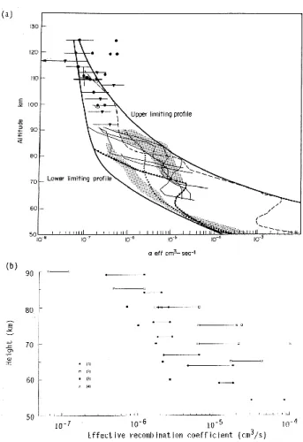
Fig. 1. Values of effective recombination coefficient determined by various methods. (a) A collection by Penman et al. (1979). (b) Recent determinations by incoherent scatter radar (Hunsucker and Hargreaves, 2003). (1) Daytime, summer, the range of values over several days (Reagan and Watt, 1976). (2) Daytime, winter, the range of values over three hours near local noon (Hargreaves et al., 1987). (3) Daytime, spring, afternoon (Hargreaves et al., 1993). (4) Night, spring (Source as 3).

depends on Ne.a, where “a” is the “specific absorption”

de-fined as the absorption per unit path at unity electron density, usually quoted in units of dB.cm3.km−1. Hence, the total ab-sorption over a vertical path is

A = Z

Ne(h).a(h).dh . (2)

The specific absorption depends on the effective collision frequency (dominated by the electron-neutral collision fre-quency ν) and the radio frefre-quency (ω) at which the absorp-tion is measured, in proporabsorp-tion to ν/(ν2+ω2). Here, ω is the angular frequency (=2π f where f is in Hz). The specific absorption may be calculated from an atmospheric model. The values used were based on the curves given by Little et al. (1964). No account is taken of possible transitory varia-tions of “a” due, for instance, to frictional heating. The ri-ometer technique (in the context of auroral absorption) has been reviewed by Hargreaves (1969).

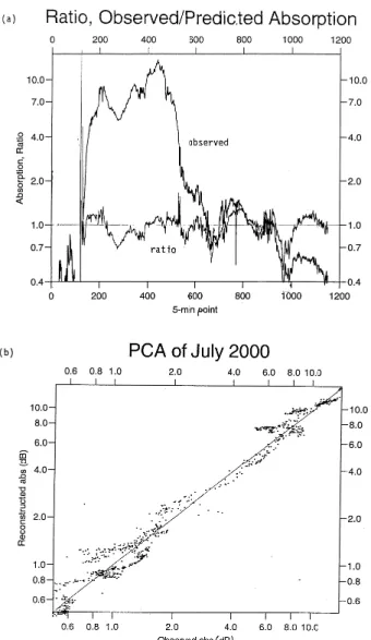
Fig. 2. Comparison between measured and calculated absorption during PCAs (Patterson et al., 2001). The outer lines indicate a difference of 20%.

J. K. Hargreaves: Polar-cap absorption events 11

Penman, J. M., Hargreaves, J. K., and McIlwain, C. E.: The re-lationship between 10 to 80 keV electrons observed at geosyn-chronous orbit and auroral radio absorption observed with riome-ters, Planet. Space Sci. 27, 445–451, 1979.

Reagan, J. B. and Watt, T. M.: Simultaneous satellite and radar studies of the D-region ionosphere during the intense solar par-ticle events of August 1972, J. Geophys. Res. 81, 4579–4596, 1976.

Reid, G. C.: Polar-cap absorption – Observations and theory, Fun-damentals of Cosmic Physics 1, 167–200, 1974.

Table 5.

Height (km)

√

Production rate Combined coeff. Absorption increment 90 √q₁₇ c17 δA17 85 √q₁₆ c16 δA16 5(n+1) √q_n cn δAn 15 √q₂ c2 δA2 10 √q₁ c1 δA1 Acalc

Reid, G. C.: Solar energetic particles and their effects on the terres-trial environment, in: Physics of the Sun, Vol III, Astrophysics and Solar-Terrestrial Relations, edited by Sturrock, P. A., Holzer, T. E., Mihalas, D. M., and Ulrich, R., D. Reidel Publishing Com-pany, Dordrecht, 251–278, 1986.

Reid, G. C., Solomon, S., and Garcia, R. R.: Response of the mid-dle atmosphere to the solar proton events of August–December 1989, Geophys. Res. Lett., 18, 1019–1022, 1991.

Fig. 3. 5-km slabs used in the computation.

While the radio absorption during a PCA may be measured without difficulty, and values of the proton fluxes are readily available, these do not immediately tell us the effects at a given altitude. Direct measurements of the electron-density profile by rocket or radar are only possible in some instances, and although the incoherent-scatter technique is an attractive one for D-region studies in general, it tends to lack the sensi-tivity required for PCA studies. The problem may in princi-ple also be solved by using pre-determined values of the ef-fective recombination coefficient. There have been many es-timates of this coefficient, but since they vary greatly (Fig. 1) it is not obvious which values should be assumed.

Gledhill (1986) reviewed the literature on αe

measure-ments under various circumstances, and derived formulae for its variation with height over the range 50–90 km. The re-sults were given for different types of D-region disturbance, and the PCA results were divided into “day” and “night” ac-cording to solar zenith angles less than 92◦and greater than 98◦, respectively. Recognising the large spread, it was stated

(4)

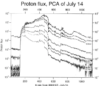
Fig. 4. Integral proton fluxes at energies exceeding 1, 5, 10, 30, 50, 60, and 100 MeV during the event which started 14 July 2000, measured by GOES-10 at geosynchronous orbit.

that the results were “not reliable to a factor of 2, and in some cases not even within an order of magnitude”. This qualification succinctly summarises our problem.

Patterson et al. (2001) used Gledhill’s profiles of effective recombination coefficient (day and night) to estimate the to-tal absorption from the observed proton spectrum in a num-ber of events, and obtained reasonable agreement, at least for the daytime. Figure 2 reproduces their comparison between observed and predicted absorption; lines have been added to indicate differences of 20%.

2 A new approach

The new approach is as follows. From Eqs. (1) and (2), we can write, A = Z q1/2.c.dh , (3) where c = a/α1/2e . (4)

Given that A is in decibels (dB), h in km, and a and αe are in the units stated above, the unit of c will be

dB.cm3/2.s1/2.km−1. The ionosphere is divided into 17 slabs of 5 km (Fig. 3). In each slab the incremental absorption is related to the square root of the production rate by the “com-bined coefficient”, c (equal to the specific absorption divided by the square root of the effective recombination coefficient). The production rates are computed from geosynchronous-satellite measurements of the proton fluxes by the method of Reid (Reid, 1986; Reid et al., 1991). The scheme of compu-tation is based on laboratory measurements of ionization by

Fig. 5. Ion production rates computed for heights from 20 to 90 km during the proton event of July 2000. The curves are displayed in two panels for clarity.

protons in air. Power-law approximations are fitted in sec-tions to the observed fluxes exceeding 1, 5, 10, 30, 50 and 100 MeV, and the energy deposition of individual protons is followed until the particle stops. At selected heights, in this case every 5 km, the deposition is integrated over energy and incidence angle.

The values of “c” are varied until the difference between the calculated and measured absorption is a minimum, the criterion being the sum of the squares of the difference taken over many values during the PCA event. We wish to vary c(n) to minimise the quantity

X

[(Acalc−Aobs)/Aobs]2, (5) where the summation is over time, and

Acalc=5

X

q1/2n .cn, (6)

where this summation is over all the slabs, n=1 to 17. The mathematical procedure, which is from the NAG Fortran Library, is designed for the solution of an

(5)

Fig. 6. Values of the combined coefficient, c in units of dB.cm3/2.s1/2.km−1, determined for daytime during the event of July 2000. (a) Results from 6 separate runs. (b) Results with some values fixed in advance.

over-determined set of equations (in our case 17 variables but as many as 667 equations). Starting from initial guesses, the program works in (in our case) 17 dimensions and samples with small steps, in order to determine in which direction the minimum lies. A larger step is then taken and the pro-cess repeated until a minimum is found. The method relies on the fact that the proton spectrum varies during the event, as a result of which the relative contribution by the various slabs changes with time. No solution would be possible if the spectrum were constant.

Some finesse is required in applying this method. The pro-cedure might find a local minimum which is not the best so-lution, and there might be mathematical solutions which are

Fig. 7. Comparison between observed and reconstructed absorption during the event of July 2000.

not realistic physically. For instance, we know that “c” can-not be negative and that it should vary smoothly from level to level. Thus, it was found useful to operate on different selections of data and to begin the iteration from different starting points. Moreover, because there will always be noise in the data we cannot expect a perfect solution. We are looking for the best answer that does not contradict existing knowledge and that tends to emerge with some consistency over a number of tests.

3 Daytime results

Daytime data are taken from the PCA event of July 2000. The integral proton fluxes above 7 threshold energies (Fig. 4) were measured on a geosynchronous GOES satellite, and production rates from 10 to 90 km were computed from them (Fig. 5). The radio absorption was measured throughout the event with the 38.2-MHz imaging riometer at Kilpisj¨arvi (Finland), geographic coordinates 69.05◦N, 20.79◦E, L-value 5.9, (Browne et al., 1995; Hargreaves and Detrick, 2002), taking the average absorption over the central five beams. This event exceeded 10 dB at its maximum. To main-tain accuracy, only values of at least 0.5 dB were used in de-termining combined coefficients.

Figure 6a shows the values of c determined using different data selections, and also the results of initial tests run using 8 slabs (of 10 km, centred 15–85 km height). In Fig. 6b, the central values, so determined, have been fixed in the hope of obtaining better precision at the upper and lower extremes. The medians from Fig. 6b have been taken as the working values of c for this event, and to represent daytime condi-tions.

In Fig. 7 the absorption pattern reconstructed using these coefficients is compared with the observed absorption. The ratio of observed/calculated absorption (Fig. 8a) has a me-dian value of 1.0 (horizontal line), and half of the values are within 10% of the median. The measure of agreement

(6)

Fig. 8. Comparisons between observed and reconstructed absorp-tion, July 2000 all during daytime. (a) Ratio of observed to pre-dicted absorption. (b) Reconstructed against observed absorption, showing overall linearity.

is substantially the same at all absorption levels (Fig. 8b). This is significant because of the assumption (Eq. 1) that the electron density varies with the square root of the produc-tion rate. Were that not the case, Fig. 8b would have deviated from linearity. We therefore have an independent experimen-tal confirmation of the square root law.

In order to test the more general validity of the coeffi-cients, computations and comparisons have been made for the events of 2 April, 24 September and 23 November 2001 (Fig. 9). The vertical lines mark the times when the solar el-evation is 0 and −10◦. We take 0◦as the limit of “daytime”. The prediction for the April event is low by 30%. The esti-mate is about right for the daytime sections of the September and November events, particularly on the first day in each case. (Since enhancements of the solar wind tend to reach the Earth later than the increase of proton flux, days after the first

Fig. 9. Predicted absorption for the daytime periods of the PCA events of 2001 starting 2 April, 24 September, and 23 November. The vertical lines mark the limits assumed for day and night: solar elevation angles 0 and −10◦respectively. The severe dip on the second day of the April event was caused by a burst of solar radio noise.

are more susceptible to contamination by auroral absorption, whose presence may be suggested by increased irregularity of the riometer trace.)

(7)

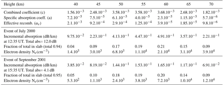
Table 1. Calculated, experimentally determined, and inferred parameters at 40–70 km during daytime PCA events.

Height (km) 40 45 50 55 60 65 70

Combined coefficient (c) 1.56.10−3 2.48.10−3 3.58.10−3 3.58.10−3 3.68.10−3 2.68.10−3 1.82.10−3 Specific absorption coeff. (a) 7.2.10−5 7.5.10−5 6.1.10−5 4.0.10−5 2.3.10−5 1.15.10−5 5.7.10−6 Effective recomb. (αe) 2.1.10−3 9.2.10−4 2.9.10−4 1.25.10−4 3.9.10−5 1.85.10−5 9.8.10−6

Event of July 2000

Incremental absorption (dB/km) 9.75.10−2 2.23.10−1 4.13.10−1 4.47.10−1 4.91.10−1 3.57.10−1 2.21.10−1 at 12:35 UT. Total abs= 12.0 dB

Fraction of total in slab (total 0.94) 0.04 0.09 0.17 0.19 0.21 0.15 0.09 Electron density Ne(cm−3) 1.4.103 3.0.103 6.8.103 1.1.104 2.1.104 3.1.104 3.9.104

Event of September 2001

Incremental absorption (dB/km) 3.85.10−2 8.19.10−2 1.44.10−1 1.53.10−1 1.65.10−1 1.17.10−1 6.91.10−2 at 15:35 UT. Total abs= 4.1 dB

Fraction of total in slab (total 0.95) 0.05 0.10 0.18 0.19 0.20 0.14 0.09 Electron density Ne(cm−3) 5.3.102 1.1.103 2.4.103 3.8.103 7.2.103 1.0.104 1.2.104

Units are c: dB.cm3/2.s1/2.km−1, a: dB.cm3.km−1, αe: cm3.s−1

4 Some inferences: incremental absorption, recombina-tion coefficient and electron density

In the July event, the incremental absorption (defined as the absorption in dB/km) comes to a maximum at 60 km dur-ing most of the event (Fig. 10), though the contributions at 55 and 50 km are as large during the early part, and the ab-sorbing layer extends well below even those levels during the growth phase (when the proton spectrum is hardest). Gener-ally, above 70 km and below 40 km the contribution to the absorption (per km) is less than 10% of that at 60 km. The slabs centred from 45 to 65 km account for 80% of the total absorption. Less that 1% of the total absorption arises below 30 km or above 80 km.

From the definition of the “combined coefficient”, c, and since we know the “specific absorption”, a, as a function of altitude, we may compute values of the “effective recombi-nation coefficient”. The most accurate values will be those for the slabs that make the largest contribution to the to-tal absorption, i.e. from 45 to 65 km. Figure 11 compares those values (extended by one slab at each end) with Gled-hill’s (1986) daytime profile of this quantity. Our values are larger by a factor of 1.5 to 2. Recall that the Gledhill values were obtained by reviewing the existing literature, in which the values show a large spread. It is interesting that the plots of Fig. 11 show similar gradients over their common height range. The new determination is entirely independent of pre-vious estimates and, moreover, it extends down to altitudes for which other data are sparse.

Specimen values of the electron density during PCA events may also be estimated from Eqs. 1, 2 and 4. Ta-ble 1 gives such values for the height range 40–70 km, for times near the daytime maxima of the events of July 2000 and September 2001. These values are consistent with di-rect measurements (by incoherent-scatter radar – Fig. 1b) at

the higher altitudes. However, no comparable radar data are believed to exist for the lower levels.

Table 1 also gives the values of combined coefficient, spe-cific absorption coefficient, and effective recombination co-efficient, all for daytime conditions as derived from the event of July 2000.

5 Night-time results

We expect the results to be rather different for the night pe-riods, when free electrons are removed at the lower altitudes by attachment to neutral species. Night periods were se-lected from the events of 23 November 2001 and 24 Septem-ber 2001, the criterion for “night” being that the Sun was more than 10◦below the horizon, this being the depression angle for which riometers generally indicate that the transi-tion to night-time absorptransi-tion levels is complete. Data from 2 April were not included because the absorption values fell below 0.5 dB. To obtain the greatest range of the proton spec-trum, we wish to include observations early and late in the event. The first phase, however, tends to be of short duration, whereas the last will be more subject to auroral contamina-tion. This is a greater problem by night than by day because the component of absorption due to the protons is relatively smaller by night for a given proton flux.

It was indeed found that the consistency of results from different runs of the procedure was poorer by night than had been the case by day. Taking what is considered to be “a good estimate”, Fig. 12 shows the reconstruction of night periods for the events of April, September and November, compared with the observations. The November event is reproduced quite well, as is the September event except for the dip immediately after sunset. The sharp enhancement

(8)

Fig. 10. The incremental absorption (dB/km) at heights 20 to 85 km, during the PCA of July 2000, showing the contribution maximising at 50–65 km during most of the event.

Fig. 11. Effective recombination coefficients for daytime derived by the present method, compared with Gledhill’s (1986) values.

Fig. 12. Predicted absorption for the night periods of the 2002 events beginning 2 April, 24 September, and 23 November. The vertical lines are as on Fig. 9.

(9)

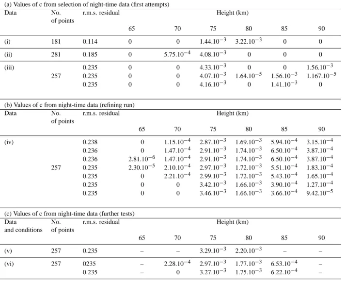
Table 2. Values of c derived from various night-time runs. (a) From three different selections of data: (i) One period in November; (ii) Periods from November and September; (iii) Three periods from November with a shorter one from September. Three progressive stages during run (iii) are shown. (b) Progressive stages of a refining run. The data set is the same as (iii), but the starting values are based on an average of the results in Table (a). (c) Further tests in which only a limited number of levels were permitted. In (v), only 75 and 80 km were allowed to be non-zero. Four levels were allowed in (vi). In each case the data set is the same as in (iii) and (iv), and the starting guess is from the bottom line of Table 2b.

(a) Values of c from selection of night-time data (first attempts)

Data No. r.m.s. residual Height (km)

of points 65 70 75 80 85 90 (i) 181 0.114 0 0 1.44.10−3 3.22.10−3 0 0 (ii) 281 0.185 0 5.75.10−4 4.08.10−3 0 0 0 (iii) 0.235 0 0 4.33.10−3 0 0 1.56.10−3 257 0.235 0 0 4.07.10−3 1.64.10−5 1.56.10−3 1.167.10−5 0.235 0 0 4.16.10−3 0 1.41.10−3 0

(b) Values of c from night-time data (refining run)

of points 65 70 75 80 85 90 (iv) 0.238 0 1.15.10−4 2.87.10−3 1.69.10−3 5.94.10−4 3.15.10−4 0.236 0 1.47.10−4 2.91.10−3 1.74.10−3 6.50.10−4 3.87.10−4 0.236 2.81.10−6 1.47.10−4 2.91.10−3 1.74.10−3 6.50.10−4 3.87.10−4 257 0.235 2.30.10−5 2.10.10−4 2.97.10−3 1.72.10−3 5.51.10−4 1.83.10−4 0.235 0 2.21.10−4 2.99.10−3 1.72.10−3 5.43.10−4 1.65.10−4 0.235 0 0 3.42.10−3 1.66.10−3 3.90.10−4 1.27.10−4 0.235 0 0 3.46.10−3 1.66.10−3 3.66.10−4 9.42.10−5

(c) Values of c from night-time data (further tests)

and conditions of points

65 70 75 80 85 90

(v) 257 0.235 – – 3.29.10−3 2.20.10−3 – –

(vi) 257 0235 – 2.28.10−4 2.97.10−3 1.77.10−3 6.53.10−4 – 0.235 – 0 3.27.10−3 1.75.10−3 6.22.10−4 –

during the September event was due to an enhancement of proton fluxes at the lower energies due to the arrival of a solar-wind shock, whose effect appeared only in the produc-tion rates above 75 km. The shape of the variaproduc-tion by night is poorly reproduced in the April event, though the absolute difference is no more than 0.3 dB.

The values of c obtained from various runs for the night periods are shown in Table 2a. The residual r.m.s. error varies only slightly between these cases, being close to 23.5%, yet the “c” values which the procedure deems to give the best fit vary widely. Evidently, the result is very sensitive to small variations in the data. On the other hand, this also means that there are several sets of “c” which will predict the absorp-tion from the proton flux equally well, presumably because

variations in the production rate are well correlated over the effective height range. Note that c=0 below 70 km in every run, which accords with the well established view that the ef-fective recombination coefficient increases sharply at sunset at the lower altitudes. The present result says that at night the radio absorption cuts off sharply below the 70 km slab and that any absorption contributions lower down are negli-gible in relation to the total. There is experimental evidence for a sharp increase in the ratio of negative ions to electrons below 75 km (Hall et al., 1988).

The first row of Table 2b is an average of the values in Table 2a, adjusted to smooth the transition between 75 and 85 km. This was then used as the starting guess and the procedure was run again, giving successively the results in

(10)

Table 3. Distribution of absorption with height at selected times in the November and September events, using coefficients from Tables 2b and c.

Set of c h (km) Incremental absorption (dB/km) % of total ab-23 November event 24 September event sorption in slab

Point Point 60 200 340 520 300 520 560 830 UT 05:00 16:40 04:20 19:20 01:00 18:20 22:40 21:10 Table 2b, 75 .075 .144 .335 .064 .081 .131 .381 .109 63–71 bottom row 80 .027 .050 .132 .029 .030 .048. .169 .051 25–39 85 .004 .008 .023 .006 .005 .008 .033 .010 4–6 90 .001 .001 .005 .000 .001 .001 .007 .002 0–1 Calculated total .54 1.02 2.48 .50 .58 .94 .2.95 .86 Observed total .52 .98 2.70 .34 .19 .71 2.34 .54 h (km) Incremental absorption Table 2c 75 .072 .135 .317 .060 .077 .124 .360 .103 59–67 bottom row 80 .029 .053 .139 .031 .031 .050 .179 .055 26–31 85 .007 .013 .039 .010 .008 .013 .056 .017 6–10 Calculated total .54 1.01 2.48 .51 .58 .94 2.98 .88 Observed total .52 .98 2.70 .34 .19 .71 2.34 .54

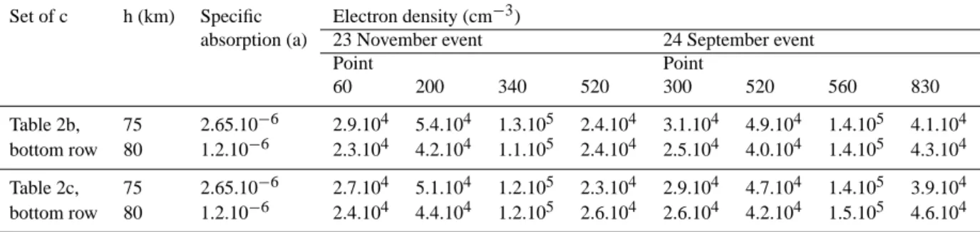
Table 4. Estimated electron densities (cm−3) at 75 and 80 km for the events and times used in Table 3.

Set of c h (km) Specific Electron density (cm−3)

absorption (a) 23 November event 24 September event

Point Point 60 200 340 520 300 520 560 830 Table 2b, 75 2.65.10−6 2.9.104 5.4.104 1.3.105 2.4.104 3.1.104 4.9.104 1.4.105 4.1.104 bottom row 80 1.2.10−6 2.3.104 4.2.104 1.1.105 2.4.104 2.5.104 4.0.104 1.4.105 4.3.104 Table 2c, 75 2.65.10−6 2.7.104 5.1.104 1.2.105 2.3.104 2.9.104 4.7.104 1.4.105 3.9.104 bottom row 80 1.2.10−6 2.4.104 4.4.104 1.2.105 2.6.104 2.6.104 4.2.104 1.5.105 4.6.104

Table 2b, the final row of which was taken as the working values for “night” in deriving the predictions in Fig. 12. Note that the change in the residual error is very slight during this run.

As a further test (Table 2c), the values of c obtained above were taken as the starting guess and only 2 levels (75 and 80 km) were allowed to generate non-zero values of c. This was repeated, allowing contributions from only 4 levels (70 to 85 km). Table 2c gives the result at 2 stages of this second run. Note that the value of c at 70 km generated in this run is either very small or zero. It was shown above that at night there are no significant contributions to the absorption from below 70 km. We can now add that when contributions are restricted to the slabs from 70 to 90 km, there are virtually no contributions from 70 or 90 km either. The night-time absorption is effectively confined to the three slabs centred from 75 to 85 km. Note that the r.m.s. residual is virtually constant in all the results shown here. Any of these sets of

coefficients will give virtually the same accuracy of PCA pre-diction (i.e. 23–24%).

6 Inferences for the night period

Table 3 gives the incremental absorption and the distribution of absorption with height for selected points (all at night) dur-ing the November and September events. The points labelled November: points 60, 200, 340 and 520; and September: points 300, 520, 560 and 830, are, respectively, at 23 Novem-ber, 05:00 UT and 16:40 UT, 24 NovemNovem-ber, 04:20 UT and 19:20 UT, 25 September 01:00 UT, 18:20 UT and 22:40 UT, and 26 September, 21:10 UT. The c values used are the fi-nal values from Table 2b, and from Table 2c, respectively. Clearly, the major part of the night-time absorption during these PCAs comes from the 75 and 80 km slabs, the former producing 60–70% of the total absorption, and the latter 25– 30%. The contribution of the 85-km slab is a minor one at

(11)

4–10% (typically in the late and early phases of the event respectively).

When it comes to estimating the effective recombination coefficients, we should, as for the daytime, only use values from slabs that make a major contribution to the total ab-sorption. For night, this restricts us to 75 and 80 km. Most of the values of c for 75 and 80 km are in the range 2.91.10−3 to 4.33.10−3and 1.66.10−3to 2.20.10−3, respectively. Fol-lowing the method of Sect. 4, these lead to values of effec-tive recombination coefficient of 8.3.10−7 to 3.7.10−7 and 5.2.10−7 _{to 3.0.10}−7_{. These values are smaller than those} from the Gledhill (1986) formula for night (1.56.10−5 _and 4.83.10−6₎_{, and are close to the “lower limiting values” in} Fig. 1 though still within the range shown there.

The values of electron density at 75 and 80 km correspond-ing to the 8 samples detailed in Table 3 are given in Table 4. We note that at these heights the electron density values are similar to each other, being about 4 to 5 times 104if the to-tal absorption is 1 dB, with approximate proportionality be-tween electron density and absorption.

7 Conclusions and discussion

The method outlined in the paper uses the variations of calcu-lated ion production rate as a function of height in compari-son with the total radio absorption measured with a riometer, to estimate the magnitude of the absorption contribution as a function of height. It has been applied to recent polar-cap absorption events, and to day and night periods separately.

Working with 5-km slabs it was found that most of the absorption occurs in the slabs centred from 45 to 65 km by day (80%), and at 75 to 80 km by night. By day, typically, less than 1% of the absorption arises above 80 km or below 30 km. At night there is no significant contribution to the absorption below the 75-km slab or at 90 km.

The observed linearity between the observed and com-puted values of total absorption provides an experimental confirmation of the square-law relationship between produc-tion rate and electron density (Eq. 1).

The method does not require values of the effective re-combination coefficient to be assumed, but estimates of this quantity may be obtained from the results. The daytime val-ues so deduced are comparable with the valval-ues recommended in Gledhill’s (1986) literature review, though they also ex-tend the range down to 40 km. Night values are considerably smaller than Gledhill’s at 75 and 80 km. Electron density val-ues may also be deduced for the heights contributing the most absorption, and these are generally comparable with results from the limited incoherent-scatter radar data available. Val-ues derived in this manner may be useful estimates at times when direct measurements are not available.

This analysis assumes that the values of the “combined coefficient”, c, are constant at a given height. In fact, there is some evidence from radar data that the effective recom-bination coefficient may vary slowly with time (Reagan and Watt, 1976; Hargreaves et al., 1993), and such a variation

would plainly reduce the accuracy of the prediction. Further, no seasonal variations have been taken into account in the present study. The method takes no account of any varia-tions in the specific absorption coefficient (Eq. 2), nor of au-roral electrons which are most likely to arrive after the first day of the proton event and have most effect at the higher al-titudes, therefore making their greatest relative contribution at night. These caveats considered, the overall accuracy of 20–25% which the method achieves appears reasonable and worthwhile.

Acknowledgements. I thank H. H. Sauer for providing the GOES proton data, G. C. Reid for the use of the procedure which com-putes production rates in the atmosphere, and J. Pritchard for indi-cating the appropriate NAG routine and explaining how to use it. The Kilpisj¨arvi imaging riometer is operated jointly by the Univer-sity of Lancaster and the Geophysical Institute, Sodankyl¨a. Some of this material was given as a poster at the Joint EGS and AGU Assembly in Nice, April 2003, and was presented verbally at the Space Weather meeting in Boulder, Colorado in May 2003.

Topical Editor M. Lester thanks E. Nielsen and another referee for their help in evaluating this paper.

References

Bailey, D. K.: Abnormal ionization in the lower ionosphere associ-ated with cosmic-ray flux enhancements, Proc. IRE 47, 255–266, 1959.

Browne, S., Hargreaves, J. K., and Honary, B.: An imaging riometer for ionospheric studies, Electron. Commun. Eng. J, 7, 209–217, 1995.

Gledhill, J. A.: The effective recombination coefficient of electrons in the ionosphere between 50 and 150 km, Radio Science 21, 399–408, 1986.

Hall, C. M., Devlin, T., Brekke, A., and Hargreaves, J. K.: Negative ion to electron number density ratios from EISCAT mesospheric spectra, Physica Scripta 37, 413–418, 1988.

Hargreaves, J. K.: Auroral absorption of HF radio waves in the ionosphere – a review of results from the first decade of riom-etry, Proc IEEE 57, 1348–1373, 1969.

Hargreaves, J. K., Ranta, H., Ranta, A., Turunen, E., and Turunen, T.: Observations of the polar cap absorption event of February 1984 by the EISCAT incoherent scatter radar, Planet. Space Sci., 35, 947–958, 1987.

Hargreaves, J. K., Shirochkov, A. V., and Farmer, A. D.: The po-lar cap absorption event of 19–21 March 1990: recombination coefficients, the twilight transition and the midday recovery, J. Atmos. Terr. Phys. 55, 857–862, 1993.

Hargreaves, J. K. and Dettrick, D. L.: Application of polar cap ab-sorption events to the calibration of riometer systems, Radio Sci-ence 37, no 3, 7–1, 7–11, doi:10.1029/2001RS002465, 2002. Hunsucker, R. D. and Hargreaves, J. K.: The high-latitude

iono-sphere and its effects on radio propagation, Cambridge Univer-sity Press, Cambridge, Chapter 7, 2003,

Little, C. G. and Leinbach, H.: The riometer – a device for the continuous measurement of ionospheric absorption, Proc. IRE 57, 315–320, 1959.

Little, C. G., Lerfald, G. M., and Parthasarathy, R.: Extension of cosmic noise absorption measurements to lower frequencies, us-ing polarized antennas, Radio Science 68D, 859–865, 1964.

(12)

J. K. Hargreaves: Polar-cap absorption events 369 Patterson, J. D., Armstrong, T. P., Laird, C. M., Detrick, D., and

Weatherwax, A.: Correlation of solar flare protons and polar cap absorption, J. Geophys. Res. 106, 149–163, 2001.

Penman, J. M., Hargreaves, J. K., and McIlwain, C. E.: The re-lationship between 10 to 80 keV electrons observed at geosyn-chronous orbit and auroral radio absorption observed with riome-ters, Planet. Space Sci. 27, 445–451, 1979.

Reagan, J. B. and Watt, T. M.: Simultaneous satellite and radar studies of the D-region ionosphere during the intense solar par-ticle events of August 1972, J. Geophys. Res. 81, 4579–4596, 1976.

Reid, G. C.: Polar-cap absorption – Observations and theory, Fun-damentals of Cosmic Physics 1, 167–200, 1974.

Reid, G. C.: Solar energetic particles and their effects on the terres-trial environment, in: Physics of the Sun, Vol III, Astrophysics and Solar-Terrestrial Relations, edited by Sturrock, P. A., Holzer, T. E., Mihalas, D. M., and Ulrich, R., D. Reidel Publishing Com-pany, Dordrecht, 251–278, 1986.

Reid, G. C., Solomon, S., and Garcia, R. R.: Response of the mid-dle atmosphere to the solar proton events of August–December 1989, Geophys. Res. Lett., 18, 1019–1022, 1991.