Development of models for the two-dimensional, two-fluid code for sodium boiling NATOF-2D

(1)

by

R. G. Zielinski and M. S. Kazimi

Energy Laboratory Report No. MIT-EL 81-030 September 1981

(2)

Energy Laboratory and

Department of Nuclear Engineering

Massachusetts Institute of Technology Cambridge, Mass. 02139

DEVELOPMENT OF MODELS FOR THE TWO-DIMENSIONAL, TWO-FLUID CODE FOR

SODIUM BOILING NATOF-2D

by

R. G. Zielinski and M. S. Kazimi

September 1981

Topical Report of the MIT Sodium Boiling Project

8

12 S . . . 0 6 0 0 13 17 17 21 1.2.1 Interfacial Mass, Energy,

and Momentum Exchange Models 1.2.2 Fluid Conduction Model . . . . 1.2.3 Direct Solution of the Pressure iel 1.2.4 Comparison to Experiments on Boiling

Behavior . . . . . . . . .

Chapter 2: INTERFACIAL MASS, ENERGY AND MOMENTUM EXCHANGE MODELS . . . . . 2.1 Introduction . . . . . . . . .. .

2.2 Conservation Equations Used in NATOF-2D 2.3 Interfacial Mass Exchange .... . . .

2.4 Energy Exchange Rate ... . . 2.5 Interfacial Momentume Transfer . . . . .

2.6 Programming Information .0 .0 . . . Chapter 3: FLUID CONDUCTION MODEL . . . . .

3.1 Introduction . . . . . . Page 21 22 22 23 24 24 26 29 40 47

54

i55 . . . . . . . . . . . . . . . . . . . . . . . . ~CI1II l~~~ ~ - - - - -. . . .

(11)

3.2 Formulation . . . .

3.3 Intercell Areas . . . . . .

3.4 Implementation Form . . . .

3.5 Experimental Calibration . . . . . . . 3.6 A Comparison with Effective Conduction

Mixing Lengths . . . .

3.7 Programming Information . . . .

Chapter 4: DIRECT SOLUTION OF THE PRESSURE FIELD 4.1 Introduction . . . .

4.2 Direct Method Solution Techniques . . 4.3 A Comparison of Direct and Iterative

Methods in NATOF-2D . . . .

4.4 Programming Information . . . . . . .

Chapter 5: EXPERIENCES WITH NATOF-2D . . . .

5.1 Introduction . . . * 5.2 Double versus Single Precision . . . .

5.3 On the Modelling of Sodium Reactors .

5.4 The Mass Exchange Rate ...

5.5 Varying Mesh Spacing . . . . . .

Chapter 6: VERIFICATION OF MODELS ...

6.1 Introduction . . . * * * * * * * 6.2 THORS Bundle 6A Experiment, Test 71H,

Run 101 * a * a a a a * * * * * , * * .

6.2.1 Description of the THORS Bundle 6A Experiment . . . . 6.2.2 Simulation Results ... . . . . . . . . . . . . . . . . . . . . . . . . . . . Page 57 61 65 68 79 87 88 88 92 . . . 97 101 102 102 103 * . . 106 . . . 109 * * . 113 * * . 115 * * • 115 * * * 116 * a * 116 * 4 & 117

(12)

-6-6.3 The W-1 SLSF Experii 6.3.1 Test Objecti Chapt Refer Apper 6.3.2 Test Apparat 6.3.3 Tests Chosen 6.4 W-1 SLSF Simulation 6.4.1 LOPI 2A . . 6.4.2 LOPI 4 . . 6.4.3 BWT 2' . . 6.4.4 BWT 7B' . .

:er 7: CONCLUSIONS AND R 7.1 Conclusions . . . 7.2 Recommendations .

ences . . . . . e * ,

idix A: SPECIFIED INLET A.1 Introduction . . o A.2 A.3 A.4 A.5 Appendix Treatment of the Mo Inlet Velocity Boun Specified Inlet Mas Condition . . . •

Programming Informa

B: NATOF-2D INPUT D

I

Appendix C: INPUT FILES FOR NATOF-2D TEST CASES C.1 Westinghouse Blanket Heat Transfer Test

Program Run 544 . . . . ... * . .

C.2 Westinghouse Blanket Heat Transfer Test Program Run 545 . . . . . . . . . .

C.3 THORS Bundle 6A Test 71H Run 101 . . . . nent . . . . . . ve . . . . us and Procedure for Simulation .. Results . . . . . . . 0 * a * * . . a 6 0 0 . 0 0 ECOMMENDATIONS . . S S * * * S * * 0 0 . a .0 0 6 0 0 0 0

VELOCITY AND MASS FL

mentum Equations dary Condition .. s Flow Rate Boundary

S 0 0 . . a 0 0 * tion . . ... ESCRIPTION . . . . 0 0 . . . . . . . . .S . . * . * *S ow * . * .S . . Page 126 126 127 127 133 133 133 138 145 151 151 153 155 157 157 159 165 167 173 174 179 179 180 181

(13)

Page C.4 C.5 C.6 C.7 Appendix Appendix Appendix Appendix W-1 SLSF LOPI 2A . . . . W-1 SLSF LOPI 4 . .. W-1 SLSF BWT 2' ... W-1 SLSF BWT 7B' . . . .

D: NATOF-2D HEXCAN MODEL . . . .

E: NATOF-2D SPACER PRESSURE DROP MODEL F: SAMPLE OUTPUT . . . . G: LISTING OF NEW NATOF-2D SUBROUTINES

* . 0 .S .. .. 00 . . . . . . . . . . . . 186 188 191 194 196 198 202

(14)

-8-List of Figures

Number Page

1.1 Typical Arrangement of Cells Used in NATOF-2D 19 2.1 Condensation Coefficient as a Function of

Pressure . . . 33 2.2 A Comparison of New and Old MasS Exchange

Rates for a Superheat of 2 C . . . 38 2.3 A Comparison of New and Old Mass Exchange

Rates for a Superheat of 20 C . . . 39 2.4 Variations between Vapor and Saturation

Temperatures for an Interfacial Heat

Transfer Nusselt Number of 0.006 .... 45 2.5 Vapor and Saturation Temperatures for an

Interfacial Heat Transfer Nusselt Number of 6.0 . . . . 46 2.6 Values of r and K as a Function of Void

Fraction for Typical Operating

Conditions . . . 51 3.1 Top View of Fluid Channels Showing the Radial

Heat Transfer Between Them . . . 58 3.2 Top View of Fluid Channels Showing Radial

Cell Boundary Numbering Scheme . . . 62 3.3 Unit Cell Used in NATOF-2D . . . 63 3.4 Radial Temperature Profile at the End of the

Heated Zone for Various Effective

Nusselt Numbers . . . 71

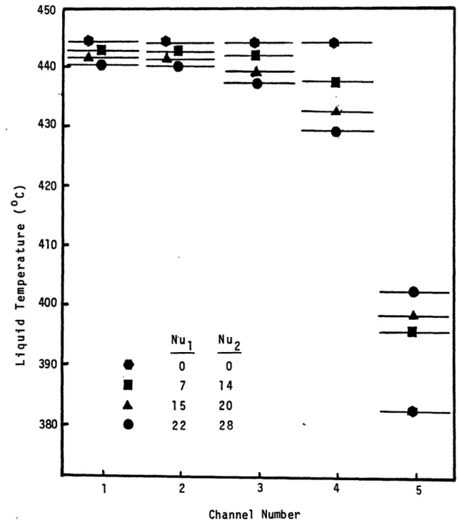
3.5 A Comparison Between Westinghouse Run 544 and NATOF-2D Radial Temperature Profiles at the Heated Zone Midplane for Nul = 22 and

Nu2 = 28 . . . . 72

3.6 A Comparison Between Westinghouse Run 544 and NATOF-2D Radial Temperature Profiles at the End of the Heated Zone for Nu

=

22

(15)

List of Figures (continued)

Number Page

3.7 A Comparison Between Westinghouse Run 544 and NATOF-2D Radial Temperature Profiles 25 Inches Downstream of Heated Zone for

Nul = 22 and Nu2 = 28 . . . e . 74

3.8 Normalized Heat Input per Rod for Westinghouse Blanket Heat Transfer Test Program

Run 545 ... * * * * * * 75

3.9 A Comparison Between Westinghouse Run 545 and NATOF-2D Radial Temperature Profiles at the Heated Zone Midplane for Nul = 22 and Nu2 = 28 . . . 76

3.10 A Comparison Between Westinghouse Run 545 and NATOF-2D Radial Temperature Profiles at the End of the Heated Zone for Nul = 22 and Nu 2 = 28 . . . . .. . . . . 77

3.11 A Comparison Between Westinghouse Run 545 and NATOF-2D Radial Temperature Profiles 25 Inches Downstream of the Heated Zone for Nul = 22 and Nu2 = 28 . . . . . . . . . 78

3.12 Possible Temperature Distributions Which Yield the Same Cell Averaged Temperature . . . 81

3.13 19-Pin Cell Geometry Used for the Calculation of Effective Mixing Lengths . . . . . . 83

4.1 Arrangement of Cells for Pressure Field Matrix Shown in Figure 4.2 . . . 89

4.2 Pressure Field Matrix . . . . . . . . . . . . 90

4.3 Upper Triangular Matrix . . . 93

4.4 Lower Triangular Matrix . . . ... 93

4.5 A Comparison of Steady State CPU Usage Between the Direct and Iterative Techniques (10 Axial Levels, 5 Radial Nodes) . . . 98

4.6 A Comparison of Transient CPU Usage Between the Direct and Iterative Techniques (10 Axial Levels, 5 Radial Nodes) . . . 99

(16)

Number Page

6.1 Location of Cells Used in the NATOF-2D

Simulation of the THORS Bundle 6A

Experiment . . . 119

6.2 NATOF-2D Predicted Inlet Mass Flow Rate of

THORS Bundle 6A Test 71H Run 101 . . . 121

6.3 NATOF-2D Temperature Profiles of Central

Channel At Various Points in Time

(THORS Bundle 6A, Test 71H, Run 101) . 122

6.4 NATOF-2D Predicted Temperature Histories at End of the Heated Zone for the Central and Edge Channels

(THORS Bundle 6A, Test 71H,Run 101) . . 123

6.5 A Comparison of NATOF-2D Predicted Liquid and Vapor and Velocities

(THORS Bundle 6A, Test 71H, Run 101) . 125

6.6 Location of Cells Used in the NATOF-2D

Simulation of the W-1 SLSF Experiments . 130 6.7 W-1 SLSF Test LOPI 2A Experiment Inlet Mass

Flow Rate / 5 / . . . 134

6.8 A Comparison Between Experiment and NATOF-2D Predicted Temperature Histories at the End of the Heated Zone for the Central

Channel (W-I SLSF Test LOPI 2A) . . . . 135

6.9 A Comparison of NATOF-2D Central and Edge

Channels Temperature Histories at the End of the Heated Zone

(W-1 SLSF Test LOPI 2A) . . . 136

6.10 W-1 SLSF Test LOPI 4 Inlet Mass Flow Rate

/ 5 / . a • . a . • • a • . . . • 137

6.11 A Comparison Between W-1 SLSF Test LOPI 4 and

NATOF-2D Temperature Histories at the

End of the Heated Zone for the Central

Channel . . . 139

6.12 A Comparison Between W-1 SLSF Test LOPI 4 and

NATOF-2D Temperature Histories at the

End of the Heated Zone for the Edge

(17)

Number Page

6.13 NATOF-2D Void Maps for W-1 SLSF Test LOPI 4 for the Central and the Middle Channels

(Void Fraction = 0.1) . . . . . . . . . 141 6.14 W-1 SLSF Test BWT 2' Inlet Mass Flow Rate . . 142 6.15 A Comparison Between W-1 SLSF Test BWT 2'

and NATOF-2D Temperature Histories at the End of the Heated Zone for the

Central Channel . . . . . . . . . . . . 143

6.16 A Comparison Between W-1 SLSF Test BWT 2' and

NATOF-2D Temperature Histories at the

End of the Heated Zone for the Edge

Channel . . . . . . . 144

6.17 A Comparison Between W-1 SLSF Test BWT 7B'

and NATOF-2D Predicted Inlet Mass Flow

Rate . . . . . 147

6.18 A Comparison of NATOF-2D Central Channel Void Maps for CF = 1.0 and CF = 0.01

(W-1 SLSF Test 7B') . . . .. 148

6.19 A Comparison of NATOF-2D Edge Channel Void Maps for CF = 1.0 and CF = 0.01

(W-1 SLSF TEst 7B') . . . . . . . . . . 149

6.20 A Comparison Between NATOF-2D and W-1 SLSF BWT 7B' Temperature Histories at the End

of the heated Zone for the Central

Channel . . . . . . . . . . . . 150

A.1 Positions Used for the Evaluation of

Variables . . . . . . . . . 161 A.2 Example Cell Numbering Scheme for Flow

Boundary Calculation . . . . . . . . . . 168 A.3 Cell Configuration for Matrix Shown in

Figure A.4 . . . . . . . 170

A.4 Pressure Field Matrix With Flow Boundary

(18)

-12-List of Tables

Number Page

2.1 Parameters Used in K versus r Comparison . . 52

3.1 Test Parameters for Westinghouse Blanket

Heat Transfer Test Program Bundle . . . . 69

3.2 Conduction Mixing Length Theory Results . . . 84

5.1 Convergence Criteria Versus Minimum Timestep

(Single Precision) . . . .a . 104

5.2 A Comparison of PWR and LMFBR Properietes . . 107

5.3 A Comparison of Water and Sodium Properties . 107

6.1 Description of THORS Bundle 6A . . .... . 118

6.2 Geometric Parameters of W-1 SLSF Test

Bundle . . . 128

6.3 Power and Flow Rates of the W-I SLSF

(19)

Nomenclature Letter a A A Ar Ar* b CF d D Dc De f g hfg h H

J

K

Units(SI)

m 2 m Definition Fuel pellet radius Area

Matrix of pressure coefficients Volumetrically averaged

Radial area between cells Radial area constant

Fuel rod radius Condensation factor Wire wrap diameter

Diameter Conductive diameter Equivalent diameter friction factor Gravity constant Enthalpy of vaporization Enthalpy

Heat transfer coefficient Mass flux

Momentum exchange coefficient

Lower triangular matrix Effective conduction mixing

length

Centroid-to-centroid distance of adjacent cells

Momentum exchange rate

m/s2 J/kg J/kg w/m2- oK kg/m2-s kg/m 3-s m kg/m 2-s L 9ij .. ij

(20)

Nomenclature (continued) Letter

M Molecular weight of particles

n Row number Nu Nusselt Number P Pressure P Fuel pitch P Perimeter q Heat flux q'" Power density q" Heat flux

Q Heat generation rate

r Radial spacial coordinate R Universal gas constant

S ij Length of common cell boundary

SBT Stable boiling timestep

t Time

T Temperature

U Velocity

U Upper triangular matrix

V Volume

w Bandwidth of matrix

W Total inlet mass flow rate

z Axial spacial coordinate

Units (SI) kg/mole N/m2 m_N/m2 m W/m 2 W/m3 W/m2 W/m m J/mole- OK m s s

OK

m/s m kg/s m

(21)

Nomenclature (continued) Greek Definition a Void fraction a Thermal diffusivity 6 Increment A Increment, spacing

r Mass exchange rate

Interfacial velocity weighting factor

p Density

a Mass exchange coefficient

Subscripts r z v i e c s T int c w Units(SI) 2 m2/s kg/m 3 -s kg/rn3 kg/m 3 Radial position Axial position Vapor Liquid Interface Evaporation Condensation Saturation Total Interface Conduction Wall

(22)

Nomenclature (continued) Superscripts

n+1 n

New time step Old time step

(23)

-17-Chapter 1 INTRODUCTION

1.1 Description of the Code

The computer code NATOF-2D was developed at the Massachusetts Institute of Technology for the simulation of both steady state and transient conditions in Liquid Metal Fast Breeder Reactors / I /. The code uses the two fluid model of conservation equations, and a two-dimensional r-z geometry which takes advantage of the symmetry found in LMFBR bundles. The two dimensional nature of the calculation allows the multidimensional effects of sodium boiling to be observed, without the corresponding high computational costs of a three dimensional code.

The model treats the liquid and vapor phases separately, coupled by only the exchange coefficients. No assumption is made about the relationship between the properties of the two phases, which allows greater generality. The method thus requires the solution of the mass, momentum and energy conservation equations for each phase.

For calculational purposes, the fuel assembly is divided into a finite number of axial and radial mess cells. There is no constraint as to the positioning or number of axial levels other than at each level the mesh spacing

(24)

remains constant. However, the boundaries between cells in the radial direction must fall between the fuel pin centerlines, and so the number of radial cells is limited to the number of fuel pin rows. Figure 1.1 shows a typical arrangement of cells used by NATOF-2D.

The fluid properties of a cell are treated as the volumetric average of the properties in that cell, which necessitates the use of sufficiently small cells in order to obtain detailed information. The fluid velocities are evaluated at the faces of the cell, and are assumed to be uniform across each cell face. The unknowns of the calculation are P, a, Tv, TZ, Uvz , Uvr , Utz , and Utr.

NATOF-2D uses a partially implicit method to solve the fluid dynamics equations. The terms involving sonic velocity and interfacial exchange are treated implicitly. However, for the convective terms, only the velocities are treated implicitly, while all other factors are evaluated at the previous timestep. This method imposes a timestep limitation such that

Az At <_- _U

Z

z

In most cases, this is not a detrimental constraint, since this timestep is usually the same order of magnitude as the time at which information is required.

The equations are solved by reduction to a Newton Iteration problem, in which the unknowns become linearized.

(25)

-19-Typical Arrangement of Cells

NATOF-2D

(26)

These equations are further reduced to a set of linear equations involving only the pressures of a cell. The pressure field is then solved for by either an iterative or a direct technique, and all variables are then updated. The advantage of using a Newton Iteration technique is that a solution can always be attained by taking a sufficiently small timestep. The heat conduction equations are solved implicitly and coupled to the fluid dydnamics equations.

The code has the capability to operate with pressure, velocity or flow boundary conditions at the inlet, and a pressure boundary condition at the outlet. The velocity and flow inlet boundary conditions are new features incorporated into NATOF-2D, and are described in Appendix A.

NATOF-2D is able to handle the most severe sodium boiling conditions, including flow reversal. The work covered in this thesis addresses some of the major difficulties encountered in past sodium boiling simulations.

(27)

-21-1.2 Scope of Work

1.2.1 Interfacial Mass, Energy and Momentum Exchange Models The constituative equations used for the calculation of the interfacial mass, energy and momentum exchange rates have been improved to more physically account for the observed phenomena. The terms have a pronounced effect on the ability of the two-fluid model to simulate sodium boiling transients, since one of the major assumptions of this work is that for void fractions below 0.957 the vapor phase does not come in contact with the wall. Thus these terms often represent the only source of mass, momentum and energy for the vapor phase.

The mass exchange rate, which has the strongest effect of any constituative relation on the running of the code, has been implemented in a more basic form than before, using the kinetic theory of condensation. It is treated in a fully implicit manner so that all dependencies on the

independent variables are accounted for. The momentum exchange rate has been modified to take into account the effects of mass exchange. Finally, the energy exchange rate has been modelled to prevent the appearance of highly subcooled vapor or superheated liquid in two phase flow transients.

(28)

1.2.2 Fluid Conduction Model

The high conductivity of liquid sodium coupled with the turbulence found in LMFBR bundles usually results in small radial temperature gradients across the core. Previously, the only mechanism available in NATOF-2D for the modelling of this phenomenon was energy exchange between cells due solely to mass transfer. However, the small radial velocities allowed large temperature differences to exist between internal channels and the edge channel.

Therefore, a radial heat conduction model has been incorporated into NATOF-2D. The model is applied only when single phase liquid is present in adjacent cells since the conductivity of the vapor phase is very low. Presently, only radial conduction has been employed in the code, since axial convection effects tend to dominate any axial conduction effects.

Calibration of the model is accomplished by simulation of two Westinghouse Blandket Heat Transfer Test Program experiments / 2 /. The model developed is also compared to analytic results based on conduction mixing length theory

/ 3 1.

1.2.3 Direct Solution of the Pressure Field

The computer time usage of NATOF-2D is strongly dependent on the solution technique used for the calculation of the pressure field. A more efficient method has been

(29)

-23-implemented into NATOF-2D which uses a direct method to solve the pressure field matrix, rather than the iterative technique previously employed. The advantages of this are substantially reduced running time, and the capability of using smaller axial mesh cell spacings.

1.2.4 Comparison to Experiments on Boiling Behavior

The major experiences encountered while running NATOF-2D are documented in Chapter 5 to serve as a

foundation for future work, and also provide an explanation for any changes deemed necessary to the previously derived models, especially the mass exchange rate. Also, some of the difficulties with sodium boiling codes in general are discussed.

Chapter 6 discusses the results obtained for five transients performed by NATOF-2D. One test was a simulation of the Thors Bundle 6A experiments conducted at Oak Ridge

National Laboratory / 4 /, while the other four are from the SLSF W-1 experiments done at the Hanford Engineering Development Laboratory / 5 /.

Finally Chapter 7 summarizes the findings of this thesis, and makes recommendations for future development of NATOF-2D.

(30)

Chapter 2

INTERFACIAL MASS, ENERGY, AND MOMENTUM EXCHANGE MODELS

2.1 Introduction

In the two fluid model NATOF-2D, each phase in the flow field is described by a set of mass, energy, and momentum equations. Each of these equations takes into account the interactions which occur between the phases. This is accomplished by the use of empirical correlations or simple physical models, that describe the mass, energy and momentum exchange rates at the liquid/vapor interface.

One of the requirements of two phase flow modelling is that no mass, energy, or momentum be gained or lost at the interface. This is the so called "jump condition" at the interface. This requirement is met if the conservation equations of each phase can be summed together, and the interface exchange terms cancel each other.

For the sodium boiling transients which NATOF-2D was designed to simulate, these exchange rates take on a special significance. One of the basic assumptions of this work is that only the liquid phase is in contact with the wall for values of void fraction up to 0.957. Thus, for many applications, the vapor phase is entirely dependent on the liquid phase as a mass, energy or momentum source, and

(31)

thereby dependent on the accuracy of the exchange models incorporated into this code.

This chapter will cover the models developed for interfacial transport exchange, and compare the results with those previously used in NATOF-2D / 1 /.

(32)

-26-2.2 Conservation Equations Used in NATOF-2D

Since this chapter deals with the modelling of the interfacial mass, enegy and momentum exchange rates, the conservation equations in the form used by NATOF-2D are summarized in this section. Since NATOF-2D is a two-phase, two-dimensional R-Z code, for each phase there will be one mass and one energy conservation equation, and two momentum equations (one for each direction) at each node. Given below are the eight conservation equations written in control volume form.

Mass Conservation liquid phase:

- f(l-a)p dV +

j

- (l-a)p UzdA + - (1-a)p U rdA

v Az+ Az_ Ar+

Ar-= - dV _(2.1)

V

vapor phase:

ap dV

ap U dA

vUv

-

ap

U dA

at v v vz f vr

v AZ+ Az_ Ar+

(33)

Conservation liquid phase:

(1-a)p (eZ + U2 /2)dV + _- _{(1-a) pU(e}

Az+ AZ-+ U /2)dA k + U /2)dA k Ar = fQdV- f(l-a) v V p gU zdV i U" f*zdA A w P•n-U dA P, + P

TF

dV -

j

qZidA A i vapor phase ap v(e _v S- _aPv_U_vr(e Ar+ Ar-Momentum + U 2/2)dV V

+

A + U /2)dA = v

-

fa

z+ Az-Q dV -dV at PVUz(eV + U V2/2)dA

f

p gU vdV V + I qVi dA Ai Conservation--Axial Direction liquid phase t (l-)pUtzdV +

I

- I(1-a)Pk UzU rdA

-Ar+

Ar-I

- 2)dA - (-) p U£zdA Az+ Az-P-k*- dA = fkzdA -AR _A w (1-a)p g Energy Ar+ (2.3) -f dA + jP'n*U dA (2.4)

-

(

l-a)pzUkr(ek

-

fP

dV -

f

M zdV (2.5)

(34)

-28-vapor phase -4apvUvzdV + V

J

PdA

ap U

2c

+ -A Az- A Az+ Az_{_} _Ar+ vUvz U vr dA -A

r-f

Pek*n dA = -fvzdA -

f

pvgdV + A Aw v

Momentum Conservation--Radial Direction liquid phase _lt-(l-a)p ZUrdV + -v _Az+ - f(l-a)p Ur dA -Ar+ Ar_{_}

-f f rdA + f M rdV

Aw v vapor phase a PvUvrdV ₊ V

(1l-a)ptUrUtzdA

+

A

z-SPr*n

dA = (2.7)

- fvUvz vrdA + - ap vU2 dA

Az+ A_{z_} _Ar+

Ar-- P.r-n dA = fvr dA -

i

MvrdV

Av _v Aw _w v

(2.8)

f MvzdV

(35)

2.3 Interfacial Mass Exchange

In the mass conservation equations for the liquid and vapor phase (equations 2.1 and 2.2) r represents the mass exchange rate between phases, and will be defined as positive for evaporation. 1 has units of kg/m3-s. At the present time, the accepted model for the mass exchange rate is based on the kinetic theory of condensation. This model views the interaction simply as the difference between a flux of particles arriving at the interface, and a flux of particles departing from the interface. The particles are assumed to be arriving from the vapor phase, and departing from the liquid phase. When the arrival rate exceeds the departure rate, condensation is occurring. In the reverse situation, evaporation takes place and when the net flux is zero, an equilibrium condition exists. The derivation of the mass exchange rate is essentially due to Schrage / 6 /.

Using a Maxwell-Boltzmann distribution, it is possible to show that in a stationary container the mass flux of particles passing in either direction through the interface is given by:

M= 2 p

i 2rR T _(2.9)

where

ji = mass flux of phase i (kg/m 2_-s) M = molecular weight of particles

(36)

-30-R = universal gas constant

P = pressure exerted by the particles T = temperature of the particles

If there exists a progress velocity on the vapor side towards the interface such that Jv = PvVp then

M 2 P T (2.10)

where

S= e-2 + or(1 + erf#) (2.11)

V

P 2R/ (2.12)

(2RT/M) T p v(2RT/M) (.

Vp = progress velocity

At the liquid-vapor interface not all the molecules striking the surface will condense. Therefore, c is defined as the fraction of molecules striking the surface which actually do condense. In a similar manner, oe represents the ratio of the flux of molecules actually leaving the interface to the flux given by equation 2.9.

At the condensing surface, molecules are arriving at a progress flow rate pvVp, and molecules are departing the surface at a rate equivalent to that of molecules in a

(37)

stationary container. Thus the net flux towards the surface is given by:

i P P

. _2JRM 2 C _T_TeT_T-v (2.13)

If it is assume that P << 1, or in other words that the condensation rate is low, Y can be approximated by the following expression:

T / + 1

Pv( 2RT /M) T (2.14)

Substituting this into equation 2.13 yields

2 a 2fR T 2 eT

c v e (2.15)

When the two phases are in equilibrium, the net flux, j, is equal to zero, and ac = e*. Since the values of the individual coefficients in non-equilibrium systems have not been determined, it is justified to set a = ae = a,. Using this approximation the net flux becomes:

J=

2a

M

21 1J

v 2 _(2.16)

and the mass exchange rate is thus

.2a M

FP

v

F = -jA = A T_ - -1

2Mv _w(2.17)

where

(38)

The literature shows a wide variation in the value of a for sodium, ranging from a = 1.0 at low pressures to a = 0.001 at atmospheric pressures (See figure 2.1). Rohsenow / 7 /, however, attributes this variation to

the presence of non-condensible gases which tend to congregate at the interface. These gases add an additional resistance to condensation. Tests conducted on nearly gas-free systems where the flow was high show that any gases present are swept away from the interface, and a = 1.0 for all pressures.

In the models developed for NATOF-2D, it is assumed that only the liquid phase is in contact with the wall for values of void fraction up to adryout. Below this value,

all heat gains to the vapor phase are solely from the liquid phase. When the liquid phase is evaporating, the vapor phase is entering the system at the saturation temperature. Similarly, condensation occurs when the liquid phases loses heat to the wall, and becomes subcooled. The vapor phase

again condenses at the saturation temperature. Thus, for a < adryout, it is justified to set T_vto T_sand Pv to Ps in equation 2.17.

For values of a > adryout' the liquid becomes entrained in the vapor phase, and then it is the vapor which experiences the heat losses and gains. Thus for this case, T = Ts, and PP = P_s in equation 2.17. In order to obtain

(39)

Pressure Condensation Pressure Coefficient as a Function 1.0 0.1 0.01 0.001 0.01 0.1 (bar) 1.0 Figure 2.1 of I I L

(40)

-34-the correct behavior of this relation, it is necessary to reverse the sign of equation 2.17 so that in a superheated vapor environment, the entrained liquid evaporates, instead of condensing. Equation 2.30 of the next section confirms this behavior.

For the range of temperatures in which sodium boiling and condensation occurs, f Ts and T2 Ts . With this

approximation, the final form of the mass exchange rate is arrived at. S< adryout n+1 n + l _2a M _ s 2 - a

L

3HL yT

T

i

(2.18)

s S> _dryout _n+l n+1 2- a M P (2.19) s where

PV = pressure corresponding to a saturation temperature of T

Pk = pressure corresponding to a saturation temperature of TZ

Ps = system pressure

T_s = saturation temperature

A = interfacial area calculated implicitly

The formulations previously used for the mass exchange rate in NATOF-2D were:

(41)

For evaporation I'= A {P 2h ngfT - Tn+i S For condensation (p h n, T - T n+1 S= n+ (l_)n R v fg v s n+ s- T2 S

These relations were based AT/T_s _{<< 1, where AT = T,} -however, show that AT can be will be discussed in furth

interfacial areas in equations explicitly, and the term a(1 -to zero for single phase flc treats all terms implicitly eliminated the a(1 - a) term. / 8 /, and depend on the a summary of the equations us(

on the assumption that T_s . Simulations by NATOF-2D, quite large. These results ler detail in Chapter 5. The 2.20 and 2.21 were calculated a) was added to force F to go )w. The present formulation r, including the areas, and has The areas are from Wilson flow regime. The following is

a < cm A 3a 1 rm m

-

2 3 m M /D 3 (P/D)2- 7/2 r = 6. x lO1 (2.22) m (2.20) (2.21)

(42)

a < 0.55 A2₂ _D 2/3 (P/D) -(2.23) 0.55 < a < 0.65 A 3 a + b.a 3 where - a - 0.55 S-0.65 - 0.55 c = 3(A 4 3A₄ d -- --_So + c 2 + d-t 3 3A2 b = 3a - A3) - a-aA2 + a-- + 2(A ₂ ol 2 a = A2 aA2 - 2*A - A 4 ) < a < 0.957 2/3r(P/D) 2 (2/3(P/D) - 2 ITra 2/3(P/D) - T SA ₄ " _{1 -} _0.957 -36-(a < m 0.65 (2.24) 4 4 D 0.957 < a < 1.0 (2.25) A5 (2.26)

(43)

A transition regime area, A3, which is a polynomial fit

between A₂ and A4, has been added in order to keep the areas and their derivatives with respect to a continuous. A comparison was made between the previous and present mass exchange rate formulations. The system pressure used for this comparison was 2 bars, and the results are shown in figure 2.2 and 2.3 for liquid superheats of 20C and 200C respectively. The results show that the new formulation predicts a more rapid vapor production especially in high void regions. Even discounting the effects of the a(1 - a) term, the present mass exchange rate still is 2 to 4 times greater than the one previously implemented. Thus more vigorous and sustained boiling for the same superheats is expected.

(44)

-38-0.1 0.2 0.3 0.4 0.5 0.6 0.7 0.8 0.9

Void Fraction

Figure 2.2 A Comparison of New and Old Mass Exchange

Rates for a Superheat of 20C

3 10 U W 4JI X W3₀₎ C 'U U, L& U) U) 'U 102 1.0

(45)

0.1 0.2 0.3 0.4 0.5 0.6 0.7 Void Fraction

Figure 2.3 A Comparison of New and Old Mass Exchange

Rates for a Superheat of 200 C

u C-, C, ! E o, w 4.) , -C.) a u-J C, 0.8 0.9 1.0

(46)

-40-2.4 Energy Exchange Rate

Reliable constituative relations for interphase heat transfer are not available at the present time. This is due in part to the insufficient attention which this phenomenon has recieved until only recently, and also to the extreme difficulty in gathering useful data on the subject.

Starting. with the two phase energy conservation equations, equations 2.3 and 2.4, one can define an energy exchange due to the difference in temperature between the phase and the interface, and an energy exchange associated with the heat transferred by virtue of mass exchange. With this premise, the energy exchange from the liquid/vapor

interface to the vapor become

qiv = r.hvs + AiHiv(Ti - TV) (2.27)

Similarly, the energy exchange from the liquid to the liquid/vapor interface is:

.i = r*hts + AiH£I(Tz - Ti) (2.28) where

r = mass exhange rate

hvs = enthalpy of the vapor at the saturation temperature

hts = enthalpy of the liquid at the saturation temperature

(47)

H. = interface to vapor phase heat transfer coefficient

HPi = liquid phase to interface heat transfer coefficient

Since the "jump condition" at the interface requires that

qiv _£i

we have

-*h + A.H i(T - Tv) = r'hs + AiH i(T - Ts) (2.29)

Equation 2.29 can be used to solve for the mass exchange rate to yield

H. ivAi(T - T _{i )}+ H i.A(T - T_{i )}

hfg (2.30)

The above relationship shows that if Hiv and H£i were known, and if Ti was defined, the mass exchange rate would be

determined. Unfortunately, there is a lack of data on the interface heat transfer coefficients at the present time. Therefore, an alternative is to use either equation 2.27 or 2.28 and the formulation given in section 2.3 for the interfacial energy exchange rate. One cannot use equation 2.27 for the vapor energy equation and equation 2.28 for the liquid energy equation simultaneously since there would be no guarantee that the jump condition was being satisfied.

(48)

value somewhere in the range between the liquid and vapor temperatures have proven fruitless. For an interface temperature based on two infinite bodies in contact, T_i is given by the relation

T - T_i _ (kpc

)

T - TT (kpc )

(2.31) Since the conductivity and density of the liquid phase is so much greater than that of the vapor phase, solution of equation 2.31 yields Ti TR. This result would be

acceptable is T, stayed near the saturation temperature when both phases are present, but difficulties experienced in attaining a high sodium vapor condensation rate have resulted in vapor coexisting with liquid which is subcooled by as much as 1000C.

Therefore, the decision was made to set the interfacial temperature to the saturation temperature. The saturation

temperature was chosen since it is the equilibrium

temperature for a two-phase mixture, As previously stated, for values of a < adryout' the vapor gains heat solely from the liquid. In an evaporating state the assumption that Ti = Ts implies that all the liquid superheat is utilized as

latent heat for evaporation. And in a condensing state where Tk < Ts, the vapor is kept at the saturation

temperature, and all heat losses from the vapor are by

(49)

a >adryout the roles of each phase will be reversed. With this understanding, the final form of the interfacial energy exchange rate becomes:

C < dryout S= n+h + An+1 (n+1 - +1) (2.32) Svs i iv s C > adryout qi= n+1 hs + An+lHH (Tn+1 - Tn+1) (2.33) where H. Nu iv D e k H = Nu V e

The previous formulation of the interfacial heat exchange rate was

= F h + r h + AiH (T - T V )

i ehvs + chs + AiHI(T - Tv) (2.34)

This formulation effectively kept TV equal to T,, and led to

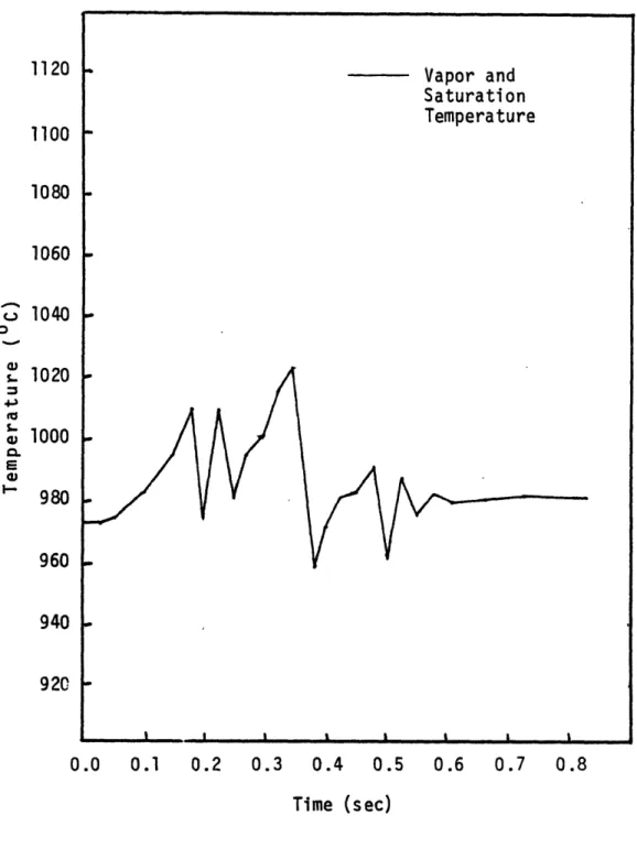
situations of the vapor phase being subcooled by as much as 1000C. The present formulation has eliminated this problem as is shown in figure 2.5.

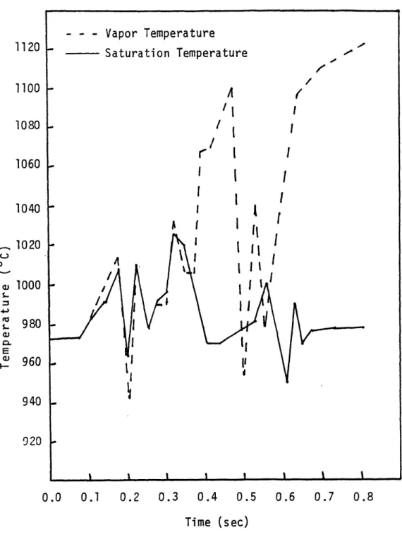
The nusselt number chosen for the interfacial heat transfer coefficients has a pronounced effect on the temperature of the phases. To illustrate this, three

(50)

simulations of a sodium boiling transient were run in which only the interfacial nusselt number was varied. In these cases there was no switch in correlations at a=adryout. The temperatures given correspond to those found at the top of the heated section of the fuel bundle. As can be seen in figure 2.4, where the vapor and liquid temperatures have been plotted versus time, a small nusselt number (Nu = 0.006) leads to quite a variation between the vapor temperature and the saturation temperature. At approximately 0.55 seconds after boiling inception, at a void fraction corresponding to adryout the vapor phase began to superheat to high levels. The liquid temperature stayed very close to the saturation temperature.

When Nu = 6, T T and T = T as figure 2.5

v s s

indicates. This test case also showed that the saturation temperature was more stable with time, and less prone to wild fluctuations. For Nu = 6000, the results were about

the same.

Based on these simulations, a value of Nu = 10 is recommended. A value in this range will keep the vapor at the saturation temperature, but not make the sensible heat contribution term the dominating one in equations 2.32 and

(51)

1120 - Saturation Temperature -1100 _A _/ r I I 1060 1040 ! 1

r

I

1020 I I cIII ' I I 1, 000 - I I I 980 -a I II S960 II 940 920 0.0 0.1 0.2 0.3 0.4 0.5 0.6 0.7 0.8 Time (sec)

Figure 2.4 Variations Between Vapor and Saturation Temperatures for an Interfacial Heat

(52)

1120 1100 1080 1060 1040 1020 1000 980 960 940 0.0 0.1 0.2 0.3 0.4 0.5 0.6 0.7 0.8 Time (sec)

Figure 2.5 Vapor and Saturation Temperatures for

an Interfacial Heat Transfer Nusselt Number of 6.0 0 03 5-4L 5-43 E 03 920

(53)

2.5 Interfacial Momentum Transfer

The interfacial momentum exchange rate, similar to the interfacial energy exchange rate, is composed of two terms. The first term takes into account the momentum gain due to mass exchange across the interface, and the second term accounts for the effect of shear stresses at the interface. This section will show how these terms can be combined into

a single term which contains both of these effects.

The momentum conservation equation for the vapor phase in the z-direction written in differential form is

(p U + (ap U2 + (ap UvrUvz) +

t Vv z vz r vz v r

a f - ap g - M_i - U_i r (2.35)

3Z

- = -fwz v.35)

where

Miz = shear stress contribution

U. i = contribution due to mass exchange which is traveling at an interfacial velocity

i = rlnu + (1 - r)Uv, where n is a weighting factor (0 I n < 1)

In order to facilitate the implimentation of the finite difference scheme utilized by NATOF-2D, it is necessary to cast equation 2.35 into non-conservative form. This is accomplished by applying the product rule of differentiation to the following terms:

(54)

Uv

-a-(ap U )_ = a+ U-(ap a

at v vz vat vzat vapv

a

(ap U2 ) = ap U

aVzp

z v vz v vz z z v vz

-(ap U U ap U au + U a (apU 3r v vz vr v vr +r vz 3r vr

Substituting these values into equation 2.35, the

(2.36)

(2.37)

(2.38)

vapor momentum equation becomes:

a p +U (ap ) + ap Uz +U (apU ) + v T - vz at v v vz -t vz az vz

vz

a

aP

apvz + U (aPUv) + a-p

-vvr vz Dr vr 3z

-f

_wz - ap g - Miz + Uizr (2.39)

The vapor mass conservation equation is given by:

v(( ₎ + -(ap vU V + (ap Uv r

(2.40) and this can be substituted into equation 2.39 to yield the non-conservative form

auvz

pV _{v at} + acp _{v vz}U _7tau vz + ap _vU _{vr ar}-a

-f - ap g - M + U iz - Uv

Next Mz is defined such that_vz

= -Miz + U iz - Uvz Vziz i. v2) vz ₊ ap a a-az (2.41) M' vt (2.42)

(55)

where

iz

: vz

Z V

- j, z)

K = interfacial momentum exchange coefficient

M' can be rearranged by the following procedure:

VZ = _{-K(Uz - U z) + [ nUz} Mz vz (1-n)U~vz - Uvz]F = -K(U - U z) + [ n(U - U v) + U v- Uv vz Ez Ezvz vz vz = -(K + Jr)*(Uvz - Uz) (2.44)

One can follow the same procedure for the liquid phase momentum equation to obtain the non-conservative form, which is: t+ (l-)j z (l-)pt 3tz + (l-a)P Uz + (1U-a)p r -z 3t Z R az S _-f _- _(l-)p _{+ Miz -} _{Uizr + U} (l-c)fr wz z) iz Rz Defining where

Mz = Miz - Uizr + Uzr

Miz

=

K*(Uvz - UZ)

one can simplify MIz to obtain

Mz = (K - (l-n)F)*(U - U z)

PIZ vz Ez

In order to better interpret these results, consider a (2.43)

(2.45)

(56)

situation where n

=

0.5 so that U = (Uz + Uv)/2, and where UV> Uk. For an evaporating condition (F > 0), the terms MIz and MIz both decrease. The vapor phase bulk momentum decreases by picking up slower particles (U_i < U_V ) and the liquid phase bulk momentum decreases by losing particles traveling at U_i > UY.

In a condensing condition, both MI and M increase. The vapor phase bulk momentum increases by losing its slow particles and the liquid phase gains momentum by receiving fast particles.

A comparison of K and nr verses void fraction was made in order to access the importance of this phenomenon. As can be seen in figure 2.6, for values of a > 0.88, the term is the dominating one. This is a desired result, since as the liquid becomes entrained in the vapor phase, the slip ratio should decrease as the liquid particles become borne in the vapor phase. Parameters used for this comparison are given in Table 2.1.

To determine what effect this modification actually has on NATOF-2D simulations, a sodium boiling transient was run with the new correlation (with n = 0.5), and compared to the same transient without it. The results showed an insignificant difference for the full range of void fractions.

Simulations were also run in which n was varied in the range from 0.0 to 1.0. The only noticeable difference was

(57)

0.0 0.1 0.2 0.3 0.4 0.5 0.6 0.7 0.8 0.9 1.0 Void Fraction

2.6 Values of r and K as a Function of Void Fraction for Typical LMFBR Transient

C,onditions 1 v, C t 4 v SL C rCI Figure

(58)

Table 2.1

Parameters Used in K versus nr Comparison

Pressure (N/m2 )

Saturation Temperature (OK) Fuel Pin Diameter (m)

Hydraulic Diameter (m) Pitch/Diameter Vapor Density (kg/m2 ) Vapor Velocity (m/s) Liquid Velocity (m/s) T - Tsat (OK) 2. x 105 1235.59 5.842 x 10 4.223 x 10-3 1.25 0.53 25.0 5.9 2.0

(59)

that for n = 0.0 the vapor velocity was lower than for n = 1.0, and for n = 0.0 the liquid velocity was higher than for n = 1.0. Since these results are for a region where condensation is occurring (r < 0), this was expected. Refering to equation 2.44, the term (K + qr) is smallest when n = 1. Thus the vapor phase isn't slowed down by the liquid phase as much. Refering to equation 2.46, the term (K - (1-)r) is smallest for r = 1, and so the liquid phase is not dragged as much by the vapor phase. Hence, the lower velocity.

(60)

2.6 Programming Information

Both the new mass exchange rate and energy exchange rate were incorporated into subroutine NONEQ.

The momentum exchange rate was incorporated into subroutine WS. Since r is required in this formulation, and since it must be evaluated at the previous time step, the value of the mass exchange rate is stored in subroutine ONESTP for use in the following time step.

(61)

-55-Chapter 3

FLUID CONDUCTION MODEL

3.1 Introduction

Some of the previous sodium boiling transients

simulated with NATOF-2D have shown a large difference in the fluid termperature between the central channels and the edge channel. A small variation is expected since the edge

channel experiences heat losses to the hexcan container, and since there is usually a lower power to flow ratio in the

ouside channel. However, whereas in the W-1 SLSF

experiments a radial temperature variation of 100C was

reported for steady state operation / 9 /, NATOF-2D

predicted a difference of 600C / 1 /.

In LMFBR bundles, the fuel rods are helically wound with spacer wires. These wires act as a spacing agent

between fuel rods, and tend to sweep the coolant

transversely around the bundle. This results in turbulence and good mixing of the coolant. NATOF-2D, as originally

developed, is unable to simulate this phenomenom. The radial velocities found in NATOF-2D are due solely to the radial pressure gradient, which in most cases is rather small in magnitude. Since mass transfer between cells was the only mechanism available for energy exchange, the large temperature gradients persisted. When boiling occurs, the

(62)

previously mentioned sweeping effects become negligible compared with the expansion of the vapor phase.

Therefore to account for the observed temperature profile, radial heat conduction has been incorporated into the code. The heat transfer between cells has been modelled in terms of "effective" conduction between the fluid in adjacent cells. Besides modelling the pure conduction effects, the formulation will also be used to account for mixing and diffusive effects in the fuel bundle. Axial heat conduction has been neglected since the the high axial velocities allow the effects of convection to dominate any conductive effects. Also, the low conductivity of the vapor phase makes any vapor-liquid or vapor-vapor radial heat transfer effects negligible. This chapter will present the methodology for calculating radial heat conduction, and offer typical values for the effective nusselt number for conduction.

(63)

-57-3.2 Formulation

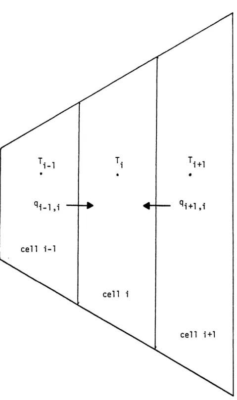
For the arrangment of cells shown in figure 3.1, the total heat transfer rate to cell i can be expressed as the sum of the heat transfer rates through each of its two faces. In this formulation, the heat flux is given by an effective heat transfer coefficient times the difference in the temperature of the adjacent cells. Written explicitly, this becomes:

qiT qi-,i + i+1,i (3.1)

where

q-,i = Ai-1,ihi-1, 1i-1

i+li Ai+liJi+li i+l

Ti)

- T_i

(3.2) (3.3) and

total heat transfer rate to cell i heat from cell i-I to cell i

heat from cell i+1 to cell i

effective heat tranxfer coefficient between cell i-1 and cell i

temperature of cell i intercell area

On either side of the interface seperating two adjacent cells, a heat transfer coefficient has been defined with the form:

qiT

=

qi-1,i

₌

qi+1,i

=

hi1,

i

=1

T

_i

₌

Ai+1,

i

=

(64)

Figure 3.1 Top View of Fluid Channels Showing the Radial Heat Transfer Between Them

(65)

-59-KR

i Nu/ 2 D (3.4)

where

Nu = effective nusselt number

KX = conductivity of the liquid in cell i

D = conductive diameter of cell i

- 4*A

P

pc = perimeter of fluid-fluid conduction

Conservation of energy.requires that the heat flux from cell i to the interface of cells i and i+1 be equal and opposite to the heat flux from cell i+1 to the interface, and so an interface temperature, Tint , can be defined such

that

hi(Tint - Ti ) = -hi+(Tint - Ti+l) (3.5)

Solving for the interface temperature yields hiT_i + hi+lTi+1

T Tint h +

h_i + hi+l _(3.6)

Since the heat flux to the interface from cell i is the same as the heat flux between cells i and i+1, the right hand side of equation 3.5 can be equated to equation 3.3 to yield:

(66)

Substituting in equation 3.6 for Tint, h can now be solved for. The result is:

i+1 hi 1+1,h h + h.

hi+1 + hi (3.8)

Considering the case where hi = hi+1, equation 3.8 reduces

to h 1/2h hi+,i 1/2hi+ KR

=

Nu---D

as one would expect.

In summary, the methodology of this approach is to calculate h as given by equation 3.4 for each cell, and then use these values to solve for hi+l,i . Once this is