ARCHVES
Discrete Cellular Lattice Assembly
MASSACHUSETTSINSTITUTEOF TECHNOLOGY
by
NOV 2.5 2015
Matthew Eli Carney
B.S.M.E., CalPoly San Luis Obispo (2004)
LIBRARIES
M.S.M.E., University of California Berkeley (2008)
Submitted to the Program in Media Arts and Sciences, School of
Architecture and Planning,
in partial fulfillment of the requirements for the degree of
Master of Science
at the
MASSACHUSETTS INSTITUTE OF TECHNOLOGY
September 2015
@
Massachusetts Institute of Technology 2015. All rights reserved.
Author...Signature
redacted
Program in Media Arts and Sciences
hl August 7, 2015Certified by....
Signature redacted...
Neil Gershenfeld
Professor of Media Arts and Sciences
Thesis Supervisor
Signature redacted
Accepted by...
...
Prof. Pattie Maes
A
mic Head, Program in Media Arts and Sciences
Discrete Cellular Lattice Assembly
by
Matthew Eli Carney
Submitted to the Program in Media Arts and Sciences, School of Architecture and Planning,
on August 7, 2015, in partial fulfillment of the requirements for the degree of
Master of Science
Abstract
Robotic assembly of discrete cellular lattices at super-hertz (>1Hz) assembly rates is shown to be possible by integrating the design of a modular robotic assembler with the specified lattice topology such that the lattice can itself be removed from the incremental assembly process. Limits to assembly rates are ultimately dependent on allowable error, system stiffness, and damping characteristics. Vibrations due to cyclical motions of the end-effector, locomotion system, and the dynamic response of an incrementally varying lattice must settle to acceptable ranges to enable engagement between end-effectors, discrete elements, and their affixing features to adjacent cells. For given system dynamics, longer settling times enables greater energy dissipation, and less error. With a greater allowable error at the interface, a shorter assembly cycle period can be attained. Passive alignment features designed into the robot end-effectors, locomotion systems, and the discrete lattice elements reduce the precision requirements of the assembly process by opening up the acceptable error range, thereby, enabling higher assembly cycle-rates. An experiment was performed to evaluate how an assembler locally referencing a lattice performed in comparison to a globally referenced assembler. The two assemblers were of similar kinematic form: both gantry-type CNC machines: a ShopBot and a custom built relative robotic assembler. The results showed superior performance by the global coordinate frame system. An error budget analysis of the two systems showed that the locally referenced, lattice based system had a larger more variable structural loop than the global coordinate frame ShopBot. The control experiment, demonstrated 0.1Hz assembly rates, while first order approximations predict a maximum 4Hz cycle for the specified interface geometry. Results show that in order to successfully assemble discrete cellular lattices at super-hertz rates the robot must itself become the local, instantaneous global coordinate frame such that the structural loop is absolutely minimized, while stiffness is maximized; at the instantaneous moment of assembly the structural loop of the robot must reference only itself.
Thesis Supervisor: Neil Gershenfeld
Discrete Cellular Lattice Assembly
This master thesis has been approved by the following committee members.
Neil Gershenfeld ...
Signature redacted
Chairman, Thesis Committee Professor of Media Arts and SciencesSignature redacted
Sangbae Kim... esis Committee
/ Membe esis Committee
Associate rofessor of c nical Engineering
Brian L. Wardle...Signature
redacted
Member, Thesis Committee Professor of Aeronautics and Astronautics
Acknowledgments
I would like to thank all of my colleagues at The Center for Bits and Atoms. Without the support of everyone it would not be possible to make cool things happen. I would
also like to thank the folks in the Program in Media Arts and Sciences for their support to help make cool things happen.
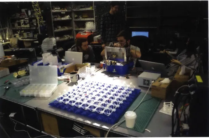
Figure 0-1: The late night crew: Sam Calisch, Will Langford, Ben Jenett, Amanda Ghassaei.
Contents
1 Introduction 17
2 Robotic Assembler Systems 21
2.1 Automated Assembly . . . . 21
2.1.1 Common Robot Classifications . . . . 21
2.1.2 Task Specific Assemblers . . . . 23
2.2 Modular Robotic Systems: Coordinated Assembly of Lattice Structures . 23 2.2.1 Brick Construction . . . . 25
2.2.2 Active Modules with Passive Truss Elements . . . . 26
2.2.3 Relative Robotic Lattice Assembly . . . . 26
2.3 G lobal vs. Local . . . . 27
3 Discrete Cellular Lattices 29 3.1 Cellular Lattice Rigidity . . . . 30
3.1.1 Kinematic Constraints . . . . 32
3.1.2 Modified Maxwell Criteria of Rigid Frameworks . . . . 33
3.1.3 Stiffness of Beams . . . . 35
3.1.4 Euler Beam Buckling . . . . 36
3.1.5 Multiphase Cellular Distribution . . . . 37
3.2 Stochastic Cellular Lattices . . . . 40
3.3 Non-stochastic Cellular Lattices . . . . 41
3.3.1 Hierarchical Structures . . . . 42
3.3.2 Kagome Structures . . . . 43
3.4 Discrete Non-Stochastic Cellular Lattices . . . . 45
4 Sources of Error 49 4.1 Static Errors . . . . 51
4.1.1 Tolerance Analysis . . . . 51
4.1.2 Total Error Budget Analysis . . . . 52
4.1.3 Elastic Averaging . . . . 55
4.2 Dynamic Error and Rate Limits . . . . 57
4.2.1 Servo Loop Time and Stiffness . . . . 58
4.2.2 Allowable Error and Frequency . . . . 59
4.2.3 P ow er . . . . 63
4.2.4 Control System . . . . 64
5 Comparable High-rate Machines 67 5.1 Qualitative Timing Analysis . . . . 67
5.2 Comparison Machines . . . . 70
6 Implementation 75 6.1 Geometries: Elements and their Interfaces . . . . 75
6.1.1 Building Blocks . . . . 77
6.1.2 Interfaces . . . . 79
6.2 Geometries: Lattice Topologies . . . . 82
6.2.1 Face Connected Octahedra . . . . 82
6.2.2 Vertex Connected Octahedra - Cuboct . . . . 85
6.2.3 Edge Connected Octahedra . . . . 88
6.2.4 K elvin . . . . 88
6.3 Robots: Designs toward dB Scaling . . . . 89
6.3.1 Gantry-based . . . . 90
6.3.2 Mandrel-based . . . . 94
6.3.3 Dynamic Aperture . . . . 95
6.3.4 Fully Passive . . . . 98
6.3.5 Hybrid Passive Dynamic . . . . 99
6.3.6 Tri-helix Locomotion Integrated . . . . 100
List of Figures
0-1 The late night crew: Sam Calisch, Will Langford, Ben Jenett, Amanda
G hassaei. . . . . 7
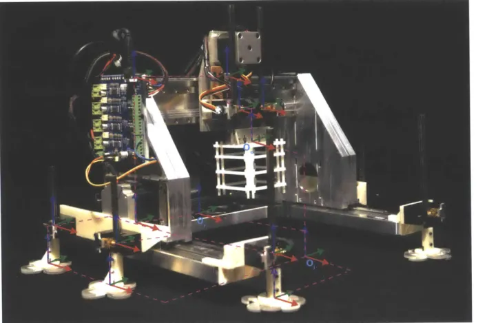
1-1 A robotic assembler of discrete cellular solids, built as a test-case to eval-uate gantry-based assembly platforms. . . . . 18
2-1 Classification of Automation, clockwise: factory automation
[1],
humanoids, robotic fabrication [2], self-assembly [3] . . . . 222-2 Task specific assemblers, counter-clockwise: space truss assembly [4], mod-ular robotic truss assembly [5], modmod-ular robotic [6], automation cell [7], filam ent winding [8]. . . . . 23
2-3 TERMES, modular brick laying robot. . . . . 25
2-4 Shady-3D reconfiguring assembler robot. . . . . 26
2-5 AMAS relative assembler robot. . . . . 27
3-1 Celluar lattices. The left-most image is a stochastic cellular lattice metal foam [9]. The right-most image is a non-stochastic discrete cellular lattice designed and built by the author. . . . . 30
3-2 (a) a mechanism; (b) a structure. . . . . 31
3-3 (a) two translations constrained, one rotation free; (b) exactly constrained two translations and one rotation. . . . . 33
3-4 Perspective sketches of assemblies to illustrate statical and kinematical determinacy and indeterminacy. . . . . 34
3-5 (a) Applied bending load; (b) applied axial load; (c) axial load sufficient to induce buckling. . . . . 36
3-6 Cubic octahedron shown as vertex connected octahedra solid phase, tiled with truncated cubic void phase. . . . . 38
3-8 Cubic octahedron coordination number . . . . 40
3-9 Hierarchical face-connected DCLA. . . . . 42
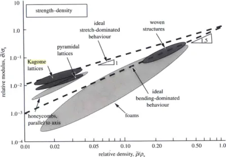
3-10 Relative modulus lattice types. . . . . 43
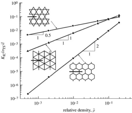
3-11 Fracture toughness of lattice types. . . . . 44
3-12 Two potential 3D Kagome lattice layouts. The connectivity remains the same, but the left image has an offset orientation which provides clean cutting planes. . . . . 44
3-13 Discrete cellular lattice assembly vocabulary. (image credit: Ben Jenett 2015) . . . .. . . . 45
3-14 Premanufactured carbon fiber laminate layup, discretely assembled into truss-core panels. Finnegan, K. A. (2007). Carbon fiber composite pyramidal lattice struc-tures. University of Virginia. [10] . . . . 45
3-15 Electronic digital materials. (image credit: Will Langford) [11] . . . . . 46
3-16 Hierarchical space structures and risk reduction from one-shot unfurling of deployable space structures. (image credit: Ben Jenett 2015) . . . . . 47
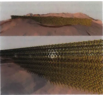
3-17 Landscape scale structures such as levees can be constructed - shown sim-ulated in the digital material design tool. [12]. (image credit: Amanda Ghassaei 2015) . . . . 48
3-18 Design tools exploiting the discretization as finite elements analysis [12]. 48 4-1 Deviations in material dimensional tolerance stack-up. . . . . 50
4-2 Coordinate frames of primary links, and their offsets for the custom built gantry-type assembler. O, is the the robot origin, 01 is the incremental local lattice origin (target location), 0e is end-effector origin. . . . . 53
4-3 Allowable error dependencies for servo-loop time and actuator stiffness. Based on equations provided by Slocum [13] . . . . 59
4-4 Spring mass model of assembly. . . . . 60
4-5 Frequency response of axial and transverse loaded beams. . . . . 62
4-6 Frequency response of an underdamped system. . . . . 63
4-7 Design space exploration of system characteristics affect on operating fre-quency, dependent on error. . . .. .... ... . .. . . . ... 63
4-8 (a)Power requirement dependencies for high frequency assembly; (b) tri-angular velocity profile. . . . . 64
5-1 One-Bit Bot, the first interpretation of a relative robotic assembler. . . . 68
5-2 High-speed industrial sewing machine. Note the large crankshaft rotation driving the needle, cast-iron frame, and the amber cooling oil tube. . . . 71
5-3 High speed bottling machinery. The KHS Innofill filling and capping ma-chines are the fastest in the industry reaching up to 80,000 bottles per hour (22Hz). Residence time is increased by passing bottles around a large circum ference. [14, 1] . . . . 71
5-4 Mass ratio of chassis frame to moving component of comparison machines. 73 6-1 Construction from pure distance and angle constraints. . . . . 78
6-2 Node-to-node connections possible with (a)vertex-connected and (b)face-connected lattice topologies. In (b) an interface geometry attempts at passive kinematic alignment: intracellular interface is ball and cone, while intercellular are tapered faces; both rely on a shear pin for tensile load. (Dimensions are 100mm node-to-node in both frames.) . . . . 79
6-3 An alignment feature that has 7r polar periodic symmetry, allows more than a millimeter of deviation in all degrees of freedom and self-energizes in compression (grid size is 1cm). The broad face, and interlocking nature of the joint enable moment coupling across the interface. . . . . 79
6-4 Joint constraints. . . . . 80
6-5 On the left is a standard issue three-groove kinematic coupling [15]."For good stability in a three-groove kinematic coupling, the normals to the planes containing the contact force vectors should bisect the angles be-tween the balls."[16] . . . . 81
6-6 (a) flat elements (PF1) with alignment features; (b) interlocking joint with additional complexity (0H5). . . . . 81
6-7 Kinematic constraints of stacked octahedra. . . . . 84
6-8 Close-up view of node interface for the octa-stack configuration. . . . . . 84
6-9 Face-connected octahedra as a volumetric lattice. . . . . 85
6-10 Mechanical testing of the octa-stack. . . . . 85
6-11 Cubic-octahedron, or vertex connected octahedra: (a) x-shape element design with shearpin; (b) square-element with clipped pins; (c) triangle-element with interlocking fingers. . . . . 87
6-12 Edge connected octahedra with kinematic constraints colored (image credit: B en Jenett) . . . . 88
6-13 Kelvin Lattice, standard discrete - left, and with reduced degrees of
free-dom, right. (node-to-node spacing is 100mm) . . . . 88
6-14 The gantry-based relative robotic assembler (designed and built in March 2015). Also shown with error budget coordinate transformations in figure 4-2 . . . . 9 0 6-15 Maximum frequency of operation with an axially loaded aluminum beam as an end-effector.. . .. . . .. ... . . . .. . . .. 93
6-16 Global positioning gantry-type assembler . . . . 95
6-17 Mandrel-based assembler . . . . 96
6-18 Rack and pinion, dynamic aperature . . . . 97
6-19 Gear tooth profile . . . . 97
6-20 The geometry of the assembly mandrel passively aligns elements during placement. Code-name: Zipper . . . . 98
6-21 A passive mandrel assembler. . . . . 99
6-22 A fully integrated locomotion, and placing system where both part place-ment, and traversal occur simultaneously. Code-name: Leapfrog . . . . . 101 6-23 A prototype of the robot arm mounted single-stage integrated octahedral
List of Tables
5.1 Individual element placement timing estimates for six discrete elements placed to form a cubic cell. . . . . 69 5.2 Timing comparison of machines with equivalent motions to assembler robots. 72
6.1 Timing estimates for both placing three elements of a cell, and simultane-ously traversing to the next cell with a passive loading mandrel. . . . . . 100 6.2 Timing estimates for both placing three elements of a cell, and
Chapter 1
Introduction
In order for robotic assemblers of discrete cellular lattices (RADCL) to reach super-hertz (>1Hz) assembly rates the system must operate with a local, instantaneous, global coordinate frame. Assembly happens without reference to the lattice, at all. The settling time for allowable error is the greatest limit to assembly rates. To reduce this error contribution the system must be maximally rigid, with minimal structural loop. There is no room for the lattice to contribute error, and so it must not. The robot incrementally ratchets along the lattice, placing cells relative to its own internal coordinate frame.
Robotic assemblers whose kinematic design is directly informed by a lattice topol-ogy exploit tuning of kinematic and inertial mechanisms for high frequency assembly and locomotion. Heterogeneous modular robotic systems, or relative robotic assembly of non-stochastic discrete cellular lattices, provide a primary contrast to traditional man-ufacturing in that the factory is turned inside out: the object being created is itself the framework for the factory; the periodic lattice acts as both the desired construction objective as well as the foundation of locomotion. It is also not self-assembly robotics, rather wherein self-assembly systems the robot is both the assembler and the structure, here, the focus is high performance lattice structures assembled by task-specific modular robots. The complexity of assembly remains within the robot, allowing the lattice to construct a material that is simple, light weight, and manufacturable at scale.
Large-scale assembly of arbitrarily sized periodic lattice structures lends itself to au-tomated assembly. This, more so than other manufacturing processes; the environment of the lattice is highly structured, enabling the automation to be equivalently structured. Where a traditional industrial robot arm provides a range of functionality, its arrange-ment of degrees of freedom and inertial characteristics generally serialize the operational
capabilities of the system. Kinematic tuning can allow parallelization of assembly se-quences while minimizing vibrational modes, thereby increasing robustness, and capacity for higher velocity construction routines. Both the robot, and the structure are defined with respect to one another, making each one a necessary, and contributing component to a heterogeneous modular robotic assembly system. Relative robotic assembly enables unbounded, repairable and reconfigurable construction, along with the computationally tuned material performance of non-stochastic discrete cellular materials. Discrete
eel-Figure 1-1: A robotic assembler of discrete cellular solids, built as a test-case to evaluate gantry-based assembly platforms.
lular lattices are a way of designing, and manufacturing with: ultralight, high stiffness material regimes [17], reuse and reconfigurability of materials [18], tuned functional per-formance [11], reduced simulation complexity [19], error correction [20], and automated assembly. Rather than building large, monolithic, single-use components, the material is discretized into simple, repeating, functional bits. A discrete set of base elements, with a discrete set of allowable positions, and orientations are integrated to form non-stochastic cellular lattices with bulk material properties. In this way, the performance of a material can be maximized by incrementally assembling high-performance sub-elements. The next element placed only after the prior, provides in situ error checking and correction. The order of magnitude difference in wavelength between discrete element, and expressed cellular solid material properties provides
JN
surface precision. The reconfigurability maximizes the sustainability post life of the product as it is simply deconstructed, and reconstructed. Finally, periodicity of structure reduces system uncertainty enablingpar-allelization of locomotion, and assembly operations.
The premise for cellular solids operation in the ultralight regime will be explained along with how the design elements necessary to generate reconfigurable discrete cel-lular lattices were identified through analysis and experimentation. The discretization allows reconfigurability of materials yet the interface between individual elements sets constraints on load paths, as well as the kinematics of assembly automation. The de-sign of the interface is directly related to the connectivity, and structural performance of the material. It is also dependent on the total static, and dynamic error budget of the assembly process; the accumulation of mechanical error from the lattice, through the assembler machine components, to the interface of the next adjoining element of the lat-tice, and the dynamic vibration of latlat-tice, and assembler all combine to define minimum clearance, and ultimately allowable interface designs. These constraints affect the mass, the stiffness of the system, and ultimately the achievable assembly rates.
By tightly integrating the design of the assembly robot along with that of the dis-cretized lattice RADCL can be optimized. As is common in robotics, the mutual inter-dependencies of the subjects must be applied to satisfy the desired goal. The breadth of this subject requires an introduction to the current state of this emerging field, which then enables an integration of those concepts into simulated, and built models.
To set the scope, similar heterogeneous reconfiguring modular robotic systems are introduced. Then, the reader is taken on a dive into cellular materials, with the intention that they surface with an appreciation for the benefits, and applications for non-stochastic discrete cellular lattices. The effects of error are so crucial to understanding the demands of the interface design -which ultimately define dynamic assembly rates -that methods of tolerance, kinematic constraint, error budget analysis, and vibrations are presented, and applied, along with a brief section discussing how elastic-averaging enables local error to become global precision. The learnings from the background chapters are then applied toward mechanical design experiments performed on lattice topologies, and their associ-ated inter, and intracellular interfaces. Rather than present all of the work I performed in this area, I provide a selection of the discovered pivotal design elements, then discuss
them through application, and simulation. 1
To test the above defined dependencies of discrete lattice assembly I built a custom, relative robotic assembler to test against an off-the-shelf, traditional, linear kinematic, gantry-type CNC machine. The question asked was: does an assembler that locally
All work performed was scaled to the same cell dimension, that being the length of an edge of a cube encompassing an octahedron: that is 100mm measured across opposing nodes on an octahedron.
references a lattice place with more or less precision than a globally referenced assembler? The experiment consisted of picking up an octahedron voxel from one location, and then placing it into a target location within an edge-connected octahedral lattice. The two machines had the same kinematic configuration consisting of linear actuators for x, y, and z axes. The dependent variable being that the custom built assembler system was mounted directly on the lattice by way of an incremental relative motion system which included leg, and foot actuators. The results of the experiment showed, that due to the increase in uncertainty from the dimensional variability accumulated from the lattice elements, a local assembler must actually be a locally global assembler.
The conclusion is that the relative robotic assembly process must minimize the struc-tural loop. The global assembler was more successful in the experiment because the tolerance stack only ever included its own, tightly controlled, and non-variable, hard-ware. In order for a robotic assembler that moves relative to the lattice to assemble locally, the assembler must minimize its structural loop; the assembler must place parts only relative to itself, without dependency on non-adjacent lattice elements. At each in-cremental step the assembler must consider that location its instantaneous global origin, and place adjacent elements with reference to only this instantaneous coordinate frame. In this way, static dimensional uncertainty is reduced, allowing more room to manage the positional variability from dynamic conditions, increasing potential assembly rates. The final chapters utilize this information, and make recommendations of designs for future relative robotic assemblers to be built and tested.
Chapter 2
Robotic Assembler Systems
The use of manipulators for assembly tasks requires that precision with which parts are positioined with respect to one another be quite high. Current ins-dustrial robots are often not accurate enough for these tasks, and building robots that are may not make sense. Manipulators of greater precision can be achieved only at the expense of size, weight, and cost. The ability to measure and control contact forces generated at the hand, however, offers a possible alternative for extending the effective precision of a manipulator. Since relative measurements are used, absolute errors in the position of the manipulator and manipulated objects are not as important as they would be in a purely position controlled system. Since small variations in relative po-sition generate large contact forces when parts of moderate sitffness interact, knowledge and control of these forces can lead to a remendous increase in effecive positional accuracy.
Craig, J. J. (1989). Introduction to robotics : mechanics and control. Read-ing, Mass. : Addison-Wesley, c1989. [21]
2.1
Automated Assembly
2.1.1
Common Robot Classifications
Robotic automation is used to perform tasks that are either unsafe for humans, or rep-etitious and require the dexterity of enough degrees of freedoms that it is not feasible to build a factory-style automation system. Common views of robots are the traditional six axis industrial robot arm, humanoid or self-assembling modular robots. The
exam-ples in figure 2-1 from top right, clockwise show traditional factory automation in a beer bottling system. The next shows a 6-axis industrial robotic arm, coupled with an additional 7th rotary axis - this robot is performing advanced computational architec-tural fabrication, it is machining custom panels for a computationally designed pavilion. Humanoid robots often have seven degrees of freedom to mimic human range of mo-tion. Humanoids are designed to operate in unstructured environments, safely, alongside humans. Self-reconfiguring Modular Robots are combinations of 1-axis modules. The reconfigurability has been partially driven by a desire to operate in unstructured envi-ronments where adaptation is necessary. These often move quite slow, and are neither good at being a robot nor a structure, but are highly adaptable.
All but one of the systems described are generalist, that is their design is such that they have a multitude of degrees of freedom to enable a variety of applications. This makes them adaptable for varying tasks, but the serial-link configuration also brings with it the additional mass of potentially unnecessary degrees of freedom. This additional mass can limit rates of motion (due to power or vibration limits), as well as limit dexterity in tight spaces. Task specific assemblers can exploit task specific kinematics.
Classification of Automation
Zykov etal 12004). MoIecbe Extended: Dlvrfing CapabltttI of Open-Source Modular Robotits OROS 2004.
Carney et al. Meka Bob**-r. 2009 Mengesetal, ICD/ aIT Research Palion 201, 5%*ga knwem4, 2Un 1
Figure 2-1: Classification of Automation, clockwise: factory automation
[1],
humanoids, robotic fabrication [2], self-assembly [3].2.1.2 Task Specific Assemblers
Hjelle, David & Upson, Hod, A Robotlca/ly Reconfigurable Truss ASME/IFToMM International
Conference on Reconfigurable Mechanisms and Robots (ReMAR), 2009.
Task Specific
Robotic Assemblers
Starltz et al. Skyworker: A Robot for Assembly, Inspection and
Maintenance of Large Scale Orbital Facllitles /ROS 200 I.
Nigl et al, Structure Reconfiguring Robots IEEE
Robotics & Automation Magazine, pp. 60-71, September 2013
Galloway et al, Factory Floor: A Robotlcally Reconfigurable Construction Platform, IEEE
lnltrnatlonal Conference on Robotics and
Automation, pp.2467-2472, 2010.
http://www.tethers.com/papers/SPACE2013_Spider Fab.pdf
Figure 2-2: Task specific assemblers, counter-clockwise: space truss assembly [4], modular robotic truss assembly [5], modular robotic [6], automation cell [7], filament winding [8].
Driving for more efficient fabrication modular reconfiguring robotic systems have been utilized to perform the specific task of assembling arbitrarily sized truss structures. Trusses are sparse, load bearing systems that are fundamentally, a set of distance and angle constraints. The system on the right is spiderbot, a space-based, in situ robotic 3D printer of large apperature trusses. Below it is a self contained filament winder for extruding composite trusses. Beside that is another type of statically mounted truss extruder that builds with distances and angles. The systems on the left crawl along the structure and assemble a truss out of discrete elements. In each case the assembly com-ponents have specific features to aid assembly. These features include passive alignment,
fixturing and even locomotion mechanisms.
2.2
Modular Robotic Systems: Coordinated
Assem-bly of Lattice Structures
One of the grand-challenges of robotics is the design and coordination of multiple robot systems to cooperatively solve tasks [22] - scalability through parallelization is the
fun-damental inspiration. A taxonomy of this new field is still subjective, and best identified by task goals rather than control architecture. Roughly, system architectures can be discretized into low-instance coordinated tasks, centralized computation with task dis-tribution, and decentralized algorithmic coordination - swarms.
Self-assembly, and re-configurable robots have been used interchangeably to describe both robots that themselves re-configure into new shapes (programmable matter [23]), and those which are able to compose, and decompose structures. This research focuses on reconfiguring robots, that is robots acting on lattice structures, but not (generally) being an integral part of the lattice. In this way the structural performance of the lattice can be maximized without massive embedded complexity. Similarly, the robotic assembler can be optimized to assembly tasks specific to the lattice topology, without the complexity of also being the lattice. The adaptability of structures is highly desirable for space-based construction where mass can be optimized for final in-space use rather than launch loading resilience - that is structural elements are packaged for launch and assembled in-space. Further, localized failures may be compensated or repaired with reconfigurable systems. Reconfigurability also allows the building of temporary scaffold structures to allow relatively simple, one-unit-step robots to assemble complex geometries such as overhangs or pillars [24]. Further, in some instances, the robot may behave as both the assembler and the structure [25], and be optimized to live, and interact only within the lattice structure [26]. Optimization between hardware, and path planning is tightly coupled due to computation, communication, topology, and physical limitations. Control strategies of swarm systems are generally based on a principle of stigmergy:
In such algorithms, local patterns of matter that result from past construction provide the exclusive cues necessary to direct and coordinate the building ac-tivities of the swarm. Therefore, any coherent architecture naturally induces coordination, which may then be seen as a by-product of the architecture; more over coordination severely constrains in turn the spaces of possible co-herent architectures. [27]
Further, a range of control strategies based on stigmergy algorithms may include such ideas of granular convection, gradients [28], etc. Most of these strategies end up being relatively similar in the fact that the agents have limited or no knowledge of overall mission goals but instead stochastically investigate, and assemble based on simple rules. While, this strategy does allow the construction of structured environments, it is done without specificity. If detailed custom configuration is necessary then a fully generalized
control approach must make use of more centralized control. Strategies range from high bandwidth communication from fully centralized computation to beacon elements that manipulate locally generalized construction.
The following is a short survey of the current state of multi-robot coordination for solving the task of assembly of discrete, cubic, lattice type structures.
2.2.1
Brick Construction
The Self-organizing Systems Research Group at Harvard University has developed a brick laying robot bioinspired by termite construction techniques, TERMES. "The hardware comprises a mobile robot and specialized passive blocks; the robot is able to manipulate blocks to build desired structures, and can maneuver on these structures as well as in unstructured environments"
[24].
The brick morphology of the structure is similar to an unstructured environment, such as a flat floor or gravel covered field. The bricks contain kinematic locating features to allow higher placement precision than the robot is, in itself, capable of providing. Similarly the bricks contain geometry to provide stepping features, locating, and communication features that provide information to the assembler robot.Control methodology is based on stigmergy with the modification that agents may be turned into beacons. This means agents, in general, follow simple rules, however, they can be locally manipulated to change their path by local beacon information. While the agents may traverse on unstructured environments, they are gravity based, and as such are constrained to assemble in ordered fashion. Temporary scaffold structures can be built to allow complex features such as pillars, and overhangs.
...
Figure 2-3: TERMES, bio-inspired construction robots.
Petersen, K. H., Nagpal, R., 6 Werfel, J. K. (2011). Termes: An autonomous robotic system for three-dimensional collective construction. In Robotics: Science and Systems Conference VII. MIT Press. [24].
2.2.2
Active Modules with Passive Truss Elements
A modular robotic system designed to not only build truss structures but to behave as active elements of the structure; Shady-3D is a three degree of freedom modular robot that is specified to live within the truss environment it constructs. Reconfigurability of the structure is a primary element of the design, such that a robotic system "decomposes a given structure into constituent building blocks and reassembles the same building blocks into a target structure... [this] approach uses truss structures rather than modular cubic units, allowing lighter structures and more flexibility in reconfiguration" [29]. Multiple assembler robots may gang themselves to increase their effective degrees of freedom for specific tasks. This research is a collaboration between the labs of Hod Lipson at Creative Machines at Cornell and Daniela Rus at the Distributed Robotics Lab at MIT. Several iterations of the robots and control algorithms have focused on topological optimization of the structures. Coordinated assembly, and activation of the structure is optimized through a quadratic competitive ratio for both static and dynamic graph methods [30].
Figure 2-4: Shady-3D, assembler robot for reconfigurable truss lattice structures.
Terada, Y., & Murata, S. (2008). Automatic Modular Assembly System and its Dis-tributed Control. The International Journal of Robotics Research, 27(3-4), 445-462. [30].
2.2.3
Relative Robotic Lattice Assembly
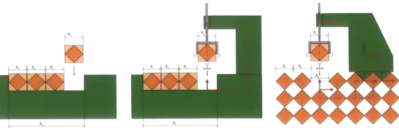
The Automatic Modular Assembly System (AMAS) is a heterogenous modular robotic construction system. The robotic assemblers are active making motions based on a finite set of required motions. The building blocks are passive cubic lattice elements, though they contain mechanisms for mechanical latching, power and communications transmission. The assemblers locate locally, relative to the structural elements of the lattice:
hands and carrying a module with its hand (L-shaped part). As any modular structure made up of these modules can be described on a cubic grid, a finite set of motion patterns is sufficient to build any shape. We took advantage of this to minimize the configuration of the assembler robot. Only four degrees of freedom are enough for locomotion and adding a new module on any surface of another. [31]
Figure 2-5: AMAS assembler robot.
Terada, Y., & Murata, S. (2006). Modular stucture assembly using blackboard path plan-ning systems. In International Symposium on Automation and Robotics in Construction
(pp. 852-857). [26]
The control strategy is gradient based; a gradient between supply chain and growth front is communicated to the assemblers to direct their motion. "The desired shape of the panel is given a priori to both the robot and the structure modules. The modules can tell whether they are at the growth front, or inside of the shape, and whether their neighbor point is occupied" [31].
2.3
Global vs. Local
Each of the above modular robotic systems utilize local reference frames for positioning and locomotion. The premise being the ability to build structures without bound. That is, by making incremental motions across the structure - assuming an effective method of material distribution - the scale of structure to be constructed is effectively unbounded. Repair, and reconfiguration of these structures is also possible with modular robots, as specific components can be reconfigured in situ, without dissassembly of monolithic components in a factory. Each of the above robotic systems operate at a scale on the order of the discrete cell size, or smaller. Each cell provides some alignment features that
provide a local position reference. The robot places components only onto the adjacent cell, and so the precision required is based on the structural loop between only adjacent cells. This provides a placing accuracy directly related to the precision of two cells.
When it comes to discrete lattice assembly, the assumption is that this local reference potentially provides higher locational precision than a global scale assembler; the error stack includes only two adjacent cells, where as global assembly includes the root sum square of all deviations between the global reference, and the end-effector. That is an end-effector, whose location is referenced to a single global origin, traversing across a vast array of cells to a target location may not find the target location in its exact, specified spot, due to the accumulation of error of each of the discrete cells. There are two possible options, then to solve this: elastic averaging, and relative placement.
It is possible to have error reduction better than linear when operating locally by exploiting elastic averaging (see 4.1.3). A modular robotic assembler that spans across
Np parts can express a local precision that is _ . For a magnitude increase in averaged accuracy it would require a span across 100 parts -perhaps unrealistic. An error reduction of one half is potentially possible with four points of contact. It should therefore be possible to utilize the concepts from modular robotic assemblers of discrete lattices to design an assembler that has higher positioning accuracy, enabling faster cycle rates (see
4.2), by utilizing a locomotion system spanning multiples cells.
Alternatively, a further reduction in error can be achieved if the lattice is actually not part of the structural loop of assembly. If, instead the robot has alignment features that enable placement only with reference to its own hardware, then the static and dynamic error contribution from the lattice can be completely removed; the robot latches onto a lattice cell, and then makes a placement maneuver into the adjacent cell by mechanically referencing its own hardware. In this way the global origin of the robot moves incrementally with the robot; at each step its instantaneous local position is its global reference frame.
Chapter 3
Discrete Cellular Lattices
Here we are concerned with lattice or cellular materials. Like the trusses and frames of the engineer, these are made up of a connected array of struts or plates, and like the crystal lattice, they are characterized by a typical cell with certain symmetry elements; some, but not all, have translational symmetry.. .At one level, they can be analysed using classical methods of mechanics, just as any space frame is analysed. But at another we must think of the lattice not only as a set of connected struts, but as a 'material' in its own right, with its own set of effective properties, allowing direct comparison with those of fully dense, monolithic materials.
Ashby, M. F. (2006). The properties of foams and lattices. Philosophical Transactions. Series A, Mathematical, Physical, and Engineering Sciences,
364(1838), p1 6. [32]
Cellular lattices, low density materials whose properties are defined by the bend-ing or stretchbend-ing of load carrybend-ing, highly connected, and sparsely distributed structures with periodic, and translational symmetries
[33]
[34] exhibit isotropic, anisotropic, or quasi-isotropic behavior determined by the connectivity of their strut node network [32].Stretch dominated axial stresses or coupled bending moments are primary material be-havior indicators that can be identified by the connectivity at nodes and the multiphase distribution of rigid and mechanism cells throughout the material [35, 36]. "For the lat-tice to behave as a material, the wavelength of any loading is also much longer than that of the lattice elements. In contrast, the lattice behaves as a 'structure' when it contains a relatively small number of lattice elements, and the length scale of the loading is comparable to that of the lattice elements" [37].
Primary engineering interest of the cellular lattice is the property of sparse density. Two distinctly different material behaviors exist within this ultralight regime: energy absorption, and stiffness [38]. Each property, unique in its cellular structure, application,
and traditionally, in its manufacturing process. Historically engineered uses of cellular solids have relied on stochastic, bending dominated cellular structures such as honeycomb
and foams, but modern manufacturing techniques enable tuned stretch dominated
non-stochastic lattices that demonstrate an order of magnitude increase in structural efficiency over bend dominated lattices [35, 39].
This research is primarily concerned with maximizing stiffness and strength of struc-tures and developing means to assemble lattices from discrete cellular components. The
following is a brief explanation of how the rigidity of a lattice framework is examined and
what underlying scaling variables exist. Then I introduce the variables of importance to
discrete cellular assembly, and how they are effected by the lattice and following chapters will explain how they effect assembly scalability.
Figure 3-1: Celluar lattices. The left-most image is a stochastic cellular lattice metal foam [9]. The right-most image is a non-stochastic discrete cellular lattice designed and
built by the author.
3.1
Cellular Lattice Rigidity
Analysis of the behavior of cellular lattices requires both a micro and a macro description. The cellular material has useful engineering mechanical properties that can be treated
as a bulk material with elastic modulus, yield strength, and mass, among other things.
These properties however, are dependent on the aggregate behavior of the cellular lattice that makes up its microstructure. The most defining attribute of the lattice is how loads are transmitted through the connecting material that forms the cells, how they connect to one another, and the distribution of cell types throughout the lattice. The nodes that are at the interface between load paths can be either exactly, over, or, under constrained.
If they are under constrained then an applied load to the lattice, such a compression or shear will cause the nodes to migrate and the connecting members to bend. If the nodes are exactly, or over constrained by the load bearing members then those same members will experience only axial, and no bending loads. This is significant because it results in an order of magnitude difference in stiffness. Perhaps the best description was given by
Deshpande et al. in the following quote and accompanying figure 3-2:
F F
joint
(a) (b)
IF F
Figure 3-2: (a) a mechanism; (b) a structure. [35]
An open-cell foam can be treated as a connected set of pin-jointed struts by the following argument. Consider the pin-jointed frames shown in Fig. 1. The frame in Fig. 1(a) is a mechanism. When loaded, the struts rotate about the joints and the frame collapses; it has neither stiffness nor strength. The triangulated frame shown in Fig. 1(b) is a structure: when loaded the struts support axial loads, tensile in some, com- pressive in others. Thus, the deformation is stretching-dominated and the frame collapses by stretching of the struts. Imagine now that the joints of both frames are frozen to prevent free rotation of the struts. On loading the first frame, the struts can no longer rotate. The applied load induces bending moments at the frozen joints, and these cause the struts to bend. This is the situation in most foam structures. However, freezing the joints of the triangulated structure has virtually no effect on the macroscopic stiffness or strength; although the struts bend, the frame is still stretching-dominated and the collapse load is dictated mainly by the axial strength of the struts.
Deshpande, V. S., Ashby, M. F., & Fleck, N. a. (2001). Foam topology: bending versus stretching dominated architectures. Acta Materialia, 49(6),
Understanding, now, that the lattice may be treated as a pin-jointed framework of struts, the traditional next step is to then evaluate the Maxwell rigidity criteria, and the coordination number for the repeating cell type. Both of these methods evaluate the kinematic constraint of lattice nodes, yet, the numerical simplifications of geometrical constraint disregards the mixture of multiphase closed polyhedra (i.e. rigid octahedron mixed with flexible truncated cubic forms) that necessarily makeup a space filling lattice, and also help define the operating behavior of cellular materials. The following section will briefly introduce kinematic constraints which apply both to the understanding of cellular lattice microstructure, rigid frameworks, as well as later will be directly applied to discrete cellular lattices.
3.1.1
Kinematic Constraints
An object can move freely in space unless constrained to not move in certain directions by some fixing force. A 2D object has three kinematic degrees of freedom two translational and one rotational: X, Y, 0,. A 3D object has six kinematic degrees of freedom three translational and three rotational: X, Y, Z, O., 0Y, 0. Structures make use of secondary rigid bodies to enforce the constraints to limit each of the degrees of freedom. Exact constraint design, or kinematic constraint design is a design methodology that aims to constrain each of the required degrees of freedom and only those required, such that additional internal stresses are not applied to the structure, and that robust, repeatable precision location of parts is possible
[40].
The methodology is straightforward. Each constraint should be effective as a strut with pins on each end, and acts along a line of action, applying tension or compression forces and no other. Only translation perpendicular to each line of action is possible. At the point of intersection of two lines of action there is a rotational degree of freedom, known as an instantaneous center of rotation. As the point of intersection approaches the limit of infinity the lines approach parallel and the rotation can be approximated as a translation. The instantaneous center of rotation is only valid at the instant of evaluation as it can migrate based on the orientation of the constraint members and their intersections. In this way, all degrees of freedom can be considered rotations. For each unwanted degree of freedom a constraint is needed to satisfy the equations of equilibrium. Further, to form a rigid body framework "each constraint line needs to have a "good size" moment arm about the instant center of rotation defined by the intersection of the other two constraint lines" [40].
The figure 3-3 shows an under constrained and exactly constrained body. The in-stantaneous center of rotation is at the intersection of each constraint line, colored light blue. In frame (a) it is apparent that x, and y are effectively constrained, yet there still exists a rotational pivot at this arbitrary location on the body shown in blue. The body is able to rotate about this point, and this point does move based on the orientation of the body. This system is a four bar linkage. Frame (b) shows a third constraint has been established that intersects with the x-axis constraint, creating a secondary instant center of rotation. This new line of action is some "good size" distance from the origi-nal instant center of (a) and generates a moment that restricts the rotatioorigi-nal degree of freedom that had existed. In this way this framework is now rigid, and each degree of freedom is exactly accounted for, it is an exact constraint design. If however, an addi-tional strut were attached to the body in (b) and it had any, even infinitesimal variation as is always the case in real systems, then all of the members would then be forced into conditions of self stress as they strain to accommodate the new, over constraint. Any infinitesimal extension in a strut due to an over constrained structure induces internal stresses throughout the structure, and is generally considered an undesirable feature in the mechanical design of structures. The following section shows how Maxwell utilized these concepts of constraint to apply towards the construction of rigid frames, and how his framework has since been utilized to predicit the behavior of cellular solids.
(a) (b)
Figure 3-3: (a) two translations constrained, one rotation free; (b) exactly constrained two translations and one rotation.
3.1.2
Modified Maxwell Criteria of Rigid Frameworks
Maxwell [41] defined the necessary conditions for a pin-jointed frame of struts to be rigid statically, and, kinematically determinate in the form a stability criteria. His method-ology later evolved into exact kinematic constraint as described above [42]. Maxwell established his rule to define the rigidity of frames, as at the time he was developing
precision instrumentation for laboratory equipment, rather than infinite frameworks of lattices. Nonetheless, it has been shown that a cellular framework can be evaluated as a system of struts, and pin joints [35]. The rules were updated to include information regarding not only if the frame was rigid, but if it is bending, or stretch dominated when the pins are effectively frozen in the nodes of a cellular lattice. The three dimensional criteria modified to examine the frame stability in terms of mechanisms and self-stress is given in the following by Pellegrino and Calladine [43]:
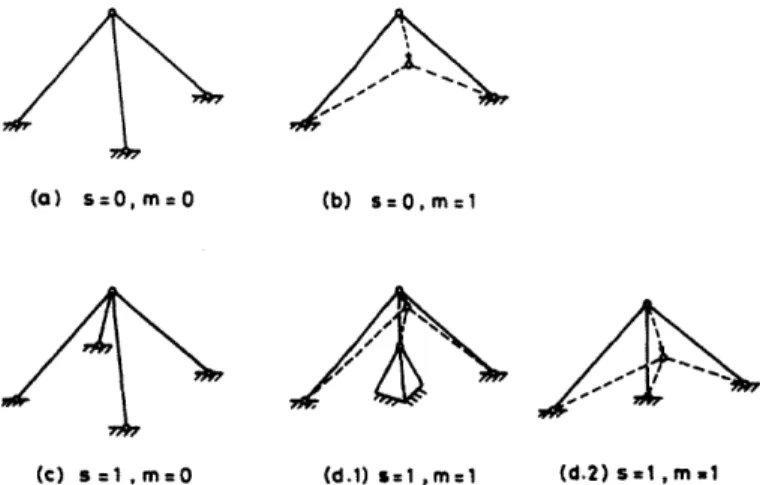
M = b - 3j+6 = s - m (3.1)
where, b is number of non-collinear struts,
j
is number of joints, s is value of self-stress, m is number of mechanisms. A visualization of what self stress and mechanisms mean in a framework is seen in figure 3-4.(a) s=O,m=O (b) s=0,m=1
(C) S=1,m =0 (d.1) s=1,m=1 (d.2) s=1,mul
Figure 3-4: "Perspective sketches of assemblies to illustrate statical and kinematical determinacy and indeterminacy. (a) The three foundation joints lie at the comers of a square. (b) One bar has now been removed, and the assembly has a mode of inextensional displacement in which the central node moves towards the reader. (c) The fourth bar makes the assembly statically in- determinate. (d.1) A third bar added to (b) makes the assembly both statically and kinematically indeterminate; but only small displacements of the inextensional mechanism are possible. (d.2) As (d. 1), except that the three foundation joints are colinear, and free motion of the inextensional mechanism, as in (b), is possible."
Pellegrino, S., & Calladine, C. R. (1986). Matrix analysis of statically and kinematically indeterminate frameworks. International Journal of Solids and Structures, 22(4), 410.
It should be noted, though, that a similar method of evaluating the behavior of cell loading conditions that commonly leads to misinterpretation of the Maxwell Criteria is
that of coordination or connectivity number, Z, that is the average number of struts connected to a node. This criteria is used as an explanation for how rigidity can be defined for an infinite lattice. From coordination number the conditions for rigidity are Z = 4 for 2D, and Z = 6 for 3D structures[43]. What is commonly forgotten, however, is that Maxwell's rule specifically states only non-collinear struts may be evaluated due to redundancy and the kinematic indeterminance of the equilibrium equations due to strut collinearity. Figure 3-7 shows a symmetrically sectioned cubic octahedron, showing how it is in fact a mechanism.
The more accurate Pellegrino and Calladine equation helps us understand the loading conditions of a cellular lattice. When M < 0, the frame is a mechanism and bending dominated. When M >= 0, the structure becomes kinematically determinate, and strut loading conditions are dominantly axial - the frame is stretch-dominated [43].
3.1.3
Stiffness of Beams
The literature has examined through empirical evaluation as well as linear algebraic anal-ysis that stretch dominated frameworks are an order of magnitude stiffer than bending dominated, and what conditions must be present in order for a lattice to exhibit such be-havior. However, one additional factor to explicitly state to help understand the scaling differences is an examination of the stiffness of a simple beam in each of these loading
conditions: axial, and transverse bending (see figure 4-4).
The distinction between stretch and bending dominated behavior can be further un-derstood by comparing the stiffness of a solid round beam in axial versus bending load conditions (figure 3-5). The mechanics for this can be found in most mechanics of mate-rials or mechanical design references[44, 45]:
ka AE (3.2)
L 3E1
kb L= (3.3)
Where, for a round slender member, d << L, and inserting
A rd 2 4 I =d
back into the stiffness equations
k AE 7E d 2 (34)
L 4 (L)
3EI 37rE d2 21
k P L 64 (L (3.5)
it can be seen that axial stiffness is related to a beam slenderness ratio d2 by an order of magnitude scaling O(c) 0
0(1). The bending stiffness of the same beam is then a
two order of magnitude 0(2) scaling of this slenderness ratio, and additionally, inversely proportional to the length of the beam.
Due to the slenderness condition of the beam this second order scaling explicitly defines the empirical evidence found by Ashby et al.[32] that bending-dominated lattices exhibit an order of magnitude less stiffness than highly triangulated stretch-dominated lattice frameworks. 4.2.2 goes into some detail of the system response to each of the axial and bending conditions.
(a) (b) (C)
Figure 3-5: (a) Applied bending load; (b) applied axial load; (c) axial load sufficient to induce buckling.
3.1.4
Euler Beam Buckling
There is a limit to the allowable slenderness ratio, and that limit is due to buckling. A long slender beam will still exhibit bending modes even in an axial load condition when the compression stress reaches a critical stress. The Euler buckling criteria for a slender beam in compression is [44]: ocr Pcr 2E (3.6) Ac ()2 r37 r =(3.7)
where, r is the radius of gyration, cr, is the critical buckling stress, I second area moment
of inertia, A projected area of beam, E modulus of elasticity, and L, is the effective length. The effective length is dependent on the constraints applied to the end conditions and can be found in the references of Hibbeler or Juvinall [44, 45]. Assuming a pin jointed constraint, this can be reorganized to evaluate the maximum effective beam length for a given geometry,
Le = r E (3.8)
Ucr
or, in the case of the simple round slender beam,
d wr2E
Le = - (3.9)
4
aOc
ac, must remain below the yield stress limit of the material, and depending on the application, should likely be further reduced to the fatigue stress limit.
For evaluation of cellular lattices it has been found that a pin joint connection be-tween struts, and nodes is an adequate representation [35]. However, what remains to be evaluated is if this effective length could be considered fixed, rather than pin-joint. For pinned joints Le = L, but for fixed end joints the theoretical limit is 2Le = L, and em-pirically 0.65Le = L. Hence, a fixed joint approximation would improve the slenderness
ratio, which theoretically cubicly improves volumetric sparsity by a half to nearly a full order of magnitude. 1
3.1.5
Multiphase Cellular Distribution
"It is worth mentioning here that any convex simply-closed polyhedron with triangular faces satisfies the Maxwell criterion and is rigid (see Appendix 9 in Calladine). It is generally assumed that the best model for a cell in a foam approximates a space filling shape. However, none of the space filling shapes (indicated by numbers 2, 3, 4, 6, 7 and 8) are rigid. In fact, we could not identify any rigid space filling cell in the 3D case and only succeeded in
10f
course, this is in contrast to the pin-jointed assumptions previously stated. Those however are approximations to simplify analysis, and it may be that each approximation can be made as appropriate and necessary for the conditions of interest - this technicality remains to be proven.
synthesising rigid periodic 3D frameworks from combinations of rigid cells (e.g. the tetrahedron and octahedron in combination fill space to form11
[32]
+
Figure 3-6: Cubic octahedron shown as vertex connected octahedra solid phase, tiled with truncated cubic void phase.
What Ashby is referring to is that while triangulated polyhedra do satisfy the Maxwell
criterion, there are only two shapes that self fill space, rigidly. In fact the only known regular polyhedra to fill space are the cube, tetrahedra, and octahedra [46]. This means,
since foams do fill space with closed polyhedra forms, there results a mixture or
multi-phase configuration of different polyhedra shapes that fill the volume. The multi-phase
arrangement may then be composed of statically rigid, fully constrained polyhedra, and polyhedra of varying mechanism.
The effective elastic moduli of such multi-phase materials are approximated by the strain energy bounds of the Hashin-Shtrikman variational principles of mixtures. Shown below is the simplification for a two phase mixture [36].
G¢ k(l-¢)+G k¢ (k
+
2G)(l - ¢)+
k (3.10) (3.11)where, ¢ is a solid volume fraction, 1 - ¢ void phase volume fraction, k bulk modulus,
ke effective bulk modulus, G shear modulus, Ge effective shear modulus [36, 47].
As the void phase volume fraction approaches zero the cellular material behaves as
its stretch-dominated rigid polyhedra dictates. However, for mixed phase cellular lattices
This derating effect can make a solid phase rigid cellular lattice and make it minimal rigid [35].
Some examples of this shown in figure 3-6 are the cubic octahedron tiling system that includes node connected octahedra (rigid), mixed with truncated cubes (mecha-nism void). The octahedron is a fully triangulated six joint, twelve strut, structure; it is exactly constrained with zero self-stress, zero mechanisms, and demonstrates stretch-dominated behaviour. The octahedron can be assembled in different density configura-tions: vertex-connected, edge-connected and face connected. Each configuration nesting with a different type of volume filling space: a truncated cube, tetrahedron and tetra-hedral dipyramid. However, as a mixture of rigid, closed polyhedra is not necessarily rigid.
In this example the octahedra are rigid, and in planar tension/compression the lat-tice remains so. However, the truncated cubic void phase volume fraction expresses three degree of freedom mechanisms (rotations about each axis). In planar shear, the vertex connected octahedra solid phase has a single constraint that lies along the plane perpen-dicular to the shear, while the void phase has a mechanism, such that the shear response of the cubic octahedra (the cuboct) comes from a pure bending load condition on the strut members of they are frozen in their joints. Another way to look at this mechanism to reference figure 3-7 where Pellegrino and Calladine demonstrate how a cross sectioned cubic octahedron can seemingly satisfy the Maxwell criteria yet be statically and kine-matically indeterminate. Finally, it is also apparent from figure 3-8 where it is clear that the node connectivity only constrains translational modes, while rotational modes are free. From this analysis we see a vertex connected, cubic octahedron has been shown to be a minimum density, maximum axially stiff lattice yet identified [17], but may only be axially stiff; it is quasitropic, axial loading is stretch dominated, shear is bending dominated.
That said, according to Deshpande et al. a rigid boundary condition can be considered part of the volume fraction, and will play a part in overall system stiffness. For instance, a rigid boundary can assert distance constraints on the boundary nodes, restricting the expression of a structural mechanism that would otherwise exist. This example surface rigidity constraint, however, becomes inconsequential as the volume increases such that the fraction of the rigid boundary condition phase becomes insignificant, and the void phase volume fraction approaches a significant contribution to the total solid volume. The system then approaches a minimal stiffness condition for the specified loading conditions