HAL Id: ensl-00338234
https://hal-ens-lyon.archives-ouvertes.fr/ensl-00338234
Submitted on 12 Nov 2008HAL is a multi-disciplinary open access archive for the deposit and dissemination of sci-entific research documents, whether they are pub-lished or not. The documents may come from teaching and research institutions in France or abroad, or from public or private research centers.
L’archive ouverte pluridisciplinaire HAL, est destinée au dépôt et à la diffusion de documents scientifiques de niveau recherche, publiés ou non, émanant des établissements d’enseignement et de recherche français ou étrangers, des laboratoires publics ou privés.
Time-Frequency Surrogates for Nonstationary Signal
Analysis
Pierre Borgnat, Patrick Flandrin
To cite this version:
Pierre Borgnat, Patrick Flandrin. Time-Frequency Surrogates for Nonstationary Signal Analysis. 8th IMA International Conference on Mathematics in Signal Processing, IMA, Cirencester, United Kingdom. �ensl-00338234�
Time-Frequency Surrogates
for Nonstationary Signal Analysis
∗Pierre Borgnat & Patrick Flandrin
Universit´e de Lyon, ´Ecole Normale Sup´erieure de Lyon
Laboratoire de Physique (UMR 5672 CNRS), 46, All´ee d’Italie, 69364 Lyon Cedex 07, France
1
Introduction
In the context of nonstationary signal analysis, especially of experimental data, a question is to give a practical meaning to what stationarity is. Indeed, whereas the theoretical concept of stationarity is well known (independence with respect to every time shifts) it cries out for an operational definition that permits to quantify if a signal is stationary or not, especially when confronted to experimental realities such as finite-length recordings, selection of relevant time-scales, statistical fluctuations in estimation,... Also, nonstationarities can take many forms: transient signals, modulations in ampli-tudes or frequencies, for stochastic or deterministic signals... Contributing to methods of assessment of stationary or nonstationary behaviors is the objective of the present work.
When dealing with one single observation, it is difficult to ascertain the significance of a stationary feature related to stationarity due to unavoidable fluctuations in estimation. We have revisited the question of stationarity testing, the framework being a comparison between local and global frequency features [1, 2]. A key ingredient is their comparison with those reproduced by some “controlled noise”, generated in a data-driven way so as to keep characteristics of the original signal (spectrum there) and scramble the one to be tested (nonstationarity)—thus providing an experimental null hypothesis for the test [1, 2, 3]. The technique of surrogate data [4, 5] can here be recognized, in a new application pertaining to stationarity, whereas surrogates were proposed initially for testing nonlinearity.
The purpose of the present communication is, after a brief outline of the use of simple surrogates as introduced so far for stationarity tests, to deal with constructions of surrogates in time-frequency domains. Indeed, for transient detection or cross-correlations analysis, one need to construct di-rectly surrogate time-frequency distributions, as opposed to distributions of surrogate time series, and keeping the ‘geometrical’ structure in the plane of the quadratic distribution.
Let us recall first basics on quadratic time-frequency distributions; they describe the evolution in time and frequency of the energy of a signal. The Wigner-Ville spectrum is a well-known solution:
Wx(t, f ) = Z +∞ −∞ E{x∗ (t − τ /2)x(t + τ /2)}e−i2πf t dτ. (1)
Better estimates (less fluctuations or oscillations) are obtained by applying some smoothing operation on Wx(t, f ). Using short-time windows hk(t), spectrograms give estimates of local frequency features:
Sx,K(t, f ) = 1 K K X k=1 Z +∞ −∞ x(s) hk(s − t) e −i2πf s ds 2 , (2)
as used in [1]. If K = 1, one recovers classical spectrograms. For K > 1 and with the K first Hermite functions, one obtains multitaper spectrograms [6] that are better estimates of the Wigner-Ville spectrum for stochastic processes, or reduced interference distribution for deterministic signals.
∗This is part of an undergoing work supported by ANR StaRAC and conducted with the collaboration of PO Amblard (GIPSA-lab, Grenoble), C Richard and P Honeine (UTT, Troyes) and J Xiao (ENS Lyon & ECNU, Shangha¨ı).
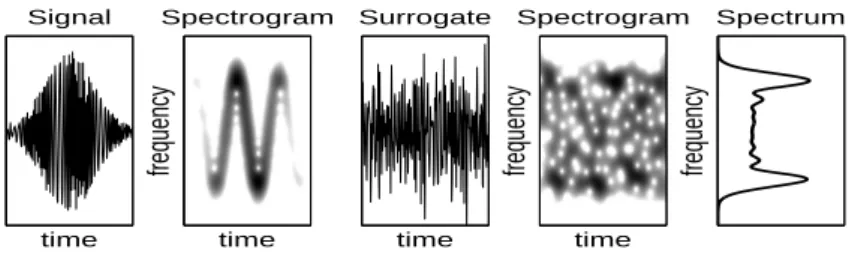
frequency Spectrum time Signal time frequency Spectrogram time Surrogate time frequency Spectrogram
Figure 1: Time-Frequency View of Surrrogates. Left to Right: a nonstationary signal; its spectrogram; a surrogate; the spectrogram of the surrogate; their common global (time-averaged) spectrum. One sees that the local frequency features, as compared to the global ones, will fluctuate more for the signals that for the surrogate which has a ’stationary’ behavior (constant in time).
Other domains of representation are used, showing the same information in different variables. The ambiguity domain is the 2D Fourier transform of Wxand reads: Ax(ξ, τ ) =R E{x∗(t − τ /2)x(t +
τ /2)}ei2πξtdt. We shall make use of it to work of surrogates in time-frequency domains.
2
Surrogate Data for Stationarity Test
An operational notion of stationarity relatively to observation time-scales is defined by the display of small fluctuations of quantities measuring a contrast between local and global frequency features [1, 2]. Global features are estimates of the marginal (in time) spectrum. Local features are estimates of the Wigner-Ville spectrum (with multitaper spectrograms). The signature of non-stationarity (and the basis of the test) is to display higher fluctuations of contrast than for stationary signals.
So as to define the null hypothesis of stationarity tests, one requires surrogates that keep un-changed the global features (time-averaged spectrum). Given that the spectum is the expectation of the squared amplitude of the Fourier transform of the signal, the simplest way is to randomize the phase of the Fourier transform of the signal (known to code the temporal features of the signal), while keeping its amplitude constant. This technique of surrogate data [4, 5] is illustrated on Fig. 1 in the time-frequency framework. Note that, up to our knowledge, it was not used before for nonstationary analysis (but for a proposal of surrogates keeping nonstationary properties for nonlinearity tests [7]). This is in a nutshell the method that we proposed, characterizing the null hypothesis of station-arity (and what “small fluctuations of contrast” mean quantitatively) through a set of surrogates drawn from the original signal. Details are to be found in [1, 2].
3
Time-Frequency Surrogates
For general nonstationarities, it is better to refine schemes for surrogates, keeping features directly the time-frequency representations. The rest of the present communication proposes an operational scheme to generate forms of surrogates defined by constraints put in time-frequency domains. Principle Classical surrogates manipulate directly the data. Our proposition is to build surrogates from its representation in a relevant time-frequency domain. The principle is to operate a direct Fourier phase randomization of the 2D representation. The details are as follows:
1. First randomize the phase in the Fourier transformed domain of the needed representation (the ambiguity domain for time-frequency representations), so that the procedure preserves its magnitude, known to be associated to the correlations and the geometry of the time-frequency distribution. 2. Additional constraints are used depending on the specific question:
– For surrogates in the time-frequency domain, as they should be of energetic nature, a positivity constraint is needed for a fair comparison of surrogates with spectrograms. Remembering that the Wigner-Ville spectrum is not always positive, we begin the procedure from spectrograms instead.
– If one wants to preserve some nonstationarity (as in [7]), but directly in time-frequency domain, one can work out the constraint in the ambiguity domain. Keeping a nonstationary variance E|x(t)|2 is achieved by constraining the ambiguity function of the surrogate on the ξ-axis to be equal to the one of the original signal, Ax(ξ, 0). The frequency marginal is constrained by the keeping of Ax(0, τ ).
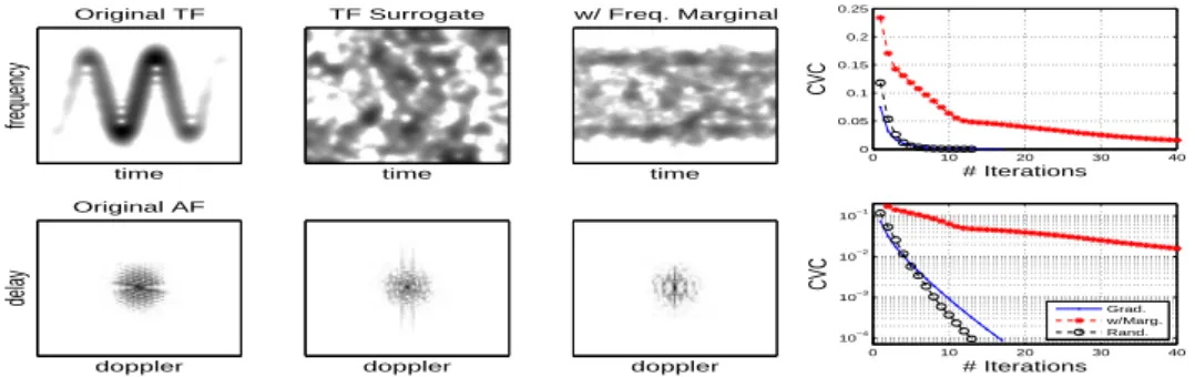
time frequency Original TF doppler delay Original AF time TF Surrogate doppler time w/ Freq. Marginal doppler 0 10 20 30 40 0 0.05 0.1 0.15 0.2 0.25 # Iterations CVC 0 10 20 30 40 10−4 10−3 10−2 10−1 # Iterations CVC Grad. w/Marg. Rand.
Figure 2: Time-Frequency Surrogates: Examples and Convergence. Spectrogram and Ambiguity function of a signal, one TF surrogate (positivity constraint) and one with also equality constraint in frequency marginal. Far right: Convergence criteria (sum of negative values divided by the sum of positive ones) vs. n.
Algorithm. The adaptation mutatis mutandis of the surrogate technique reads as follows:
(i) Do the 2D-Fourier transform of Wx(or its estimate through the multitaper spectrogram (2))
which is in the ambiguity domain;
(ii) Keep its amplitude and randomize the phase by replacing it with an admissible phase obtained as the phase of a realization of the ambiguity function of a white noise;
(iii) Come back in the time-frequency domain by inverting the Fourier transform;
(iv) Impose relevant constraints as discussed before, because they are not necessarily obtained by the previous procedure. Then, in order to keep an admissible representation, we follow the lead of [5, 8] and propose for this step an iterative method which asymptotically corrects the representation toward positivity. This method was first presented in [9], then in [3]. From step n to step n + 1, the algorithm is as follows (supposing here that only the positivity constraint is used; this can be replaced by any other one constraint):
1. Constraint: Take the positive part (S(n)(t, f ))+ of the time-frequency surrogate;
2. Compute the new ambiguity under positivity constraint: ˜A(n)(ξ, τ ) = F−1
t Ff(S(n)(t, f ))+;
3. Correct the new ambiguity by a gradient adjustment: A(n+1) = | ˜A(n)|ei(argA(n)+δϕ(n)), hence keeping the magnitude and adjusting the phase by some δϕ(n) toward an admissible one;
4. Compute the new time-frequency surrogate: S(n+1)(t, f ) = F
ξF−τ1(A(n+1)(ξ, τ ));
5. Stopping criteria: when the constraint (positivity here) is approximatively satisfied (given an a priori threshold on the negative proportion in S(n+1)(t, f )), else iterate n + 1 to the next step.
This phase correction is an iterative gradient algorithm with constraint. This correction is taken as δϕ(n)= λ(arg ˜A(n)− argA(n)) with some λ < 1, and read as:
arg(A(n+1)) = arg(A(n)) + λ(arg ˜A(n)− arg A(n)). (3) This results in convergence of the iterations toward a representation whose ambiguity function is the closest (in minimal quadratic sense) of the original randomized ambiguity function, with positivity constraint of the corresponding spectrogram and an admissible phase.
Imposing positivity and exact equality of the magnitude of the ambiguity function (on step 3 of the iterative algorithm: replace | ˜A(n)| by |A(n)|) leads to a convergence (albeit slow) to the original
distribution, up to some shift in time and frequency (which affects only the phase in the ambiguity domain). This is an evidence of the redundancy of the ambiguity representation of the signal. Convergence. We first look experimentally at the convergence of the procedure. In Fig. 2, exam-ples for time-frequency surrogates are reported with 2 different choices of constraints: 1) positivity only, 2) positivity and keeping the marginal in frequency. Numerical experiments show that the proposed procedure converges correctly (if λ is not too large, typically, λ = 0.1). However, the con-vergence is slower when constraints are added. Using surrogates for tests require to compute several realizations so as to empirically compute the null distribution, and this can be a limit. To accelerate the convergence, a second method is to use a stochastic search for the solution, inspired by simulated annealing convergence. The algorithm (proposed in [9]), uses a random correction of the phase by adding in step 3: δϕ(n)= γnarg(A
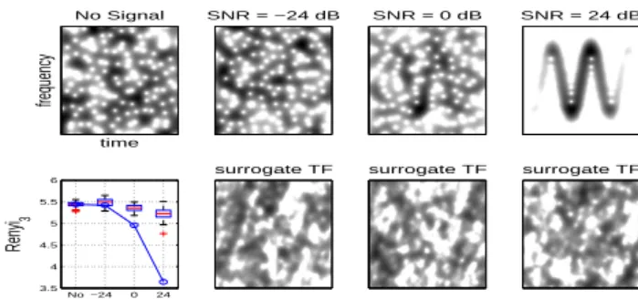
time frequency No Signal SNR = −24 dB surrogate TF SNR = 0 dB surrogate TF SNR = 24 dB surrogate TF No −24 0 24 3.5 4 4.5 5 5.5 6 Renyi 3 SNR
Figure 3: Transient Detection. A chirp is embedded in a white Gaussian noise with several SNR (-24, 0 and 24 dB); TFD of the signal and TF-surrogate with positivity constraint are shown. Bottom left: distribution of R´enyi entropy of order 3 of the surrogates (box-plot) and value for the signal (circle); as this value is lower (if transient is significant, SNR 0 or higher), as compared to TF surrogates, this test detects transients.
γ < 1. This method is found to perform particularly well in practice and converges in less steps. The price is then that convergence is not guaranteed if the original solution is further away from the target; this does not happen with positive constraint only, but it can with constraints on marginals. Example of Transient Detection. The existence of transients in a signal can then be tested using surrogates [3, 9]. Taking the R´enyi entropy of the time-frequency distribution (measuring the randomness in the time-frequency domain) as test statistics, one expect to detect a transient with a decrease of entropy if compared to equivalent, yet random, signals—thoses are provided by Time-Frequency surrogates. Fig. 3 shows an example of this test.
4
Conclusion and Perpectives
The procedure proposed here is found to work well. Because cross-spectrum and cross-ambiguity functions have definitions equivalent to the univariate case, one can create time-frequency surrogates of these quantities for testing of nonstationarities in cross-correlations (see [3]). A multivariate formulation of surrogates [10] (keeping the cross-spectrum) may be not sufficient because it keeps only the marginal but not the geometrical structure in the plane of the quadratic distribution. Also, one can wonder also whether the surrogates could be related or compared to other resampling plans (such as bootstrap, jacknife, cross-validation,. . . [11]) and this will be addressed in future works.
References
[1] J. Xiao, P. Borgnat and P. Flandrin, “Testing stationarity with time-frequency surrogates,” Proc.
EUSIPCO-07, Poznan (PL), 2007.
[2] J. Xiao, P. Borgnat, P. Flandrin and C. Richard, “Testing stationarity with surrogates – A one-class SVM approach,” Proc. IEEE Stat. Sig. Proc. Workshop SSP-07, Madison (WI), 2007.
[3] P. Borgnat, P. Flandrin, “Stationarization via Surrogates,” Journal of Statistical Mechanics: Theory and
Experiments, accepted, and expected online publication: January 2009.
[4] J. Theiler et al., “Testing for nonlinearity in time series: the method of surrogate data,” Physica D, Vol. 58, No. 1–4, pp. 77–94, 1992.
[5] T. Schreiber and A. Schmitz, “Improved surrogate data for nonlinearity tests,” Phys. Rev. Lett., Vol. 77, No. 4, pp. 635–638, 1996.
[6] M. Bayram and R.G. Baraniuk, “Multiple window time-varying spectrum estimation,”in Nonlinear and
Nonstationary Signal Processing(W.J. Fitzgerald et al., eds.), pp. 292–316, Cambridge Univ. Press, 2000.
[7] C.J. Keylock, “Constrained surrogate time series with preservation of the mean and variance structure,”
Phys. Rev. E, vol. 73, pp. 030767.1-030767.4, 2006.
[8] T. Schreiber and A. Schmitz, “Surrogate time series,” Physica D, Vol. 142, pp. 346–382, 2000.
[9] P. Flandrin, “Time-frequency surrogates,” invited talk at the AMS Joint Mathematics Meeting, San Diego, January 2008. http://perso.ens-lyon.fr/patrick.flandrin/talkAMS08 handout.pdf
[10] D. Prichard and J. Theiler, “Generating surrogate data for time series with several simultaneously mea-sured variables,” Phys. Rev. Lett., Vol. 73, No. 7, pp. 951–954, 1994.