HAL Id: hal-01021780
https://hal-enac.archives-ouvertes.fr/hal-01021780
Submitted on 27 Oct 2014
HAL is a multi-disciplinary open access
archive for the deposit and dissemination of
sci-entific research documents, whether they are
pub-lished or not. The documents may come from
teaching and research institutions in France or
L’archive ouverte pluridisciplinaire HAL, est
destinée au dépôt et à la diffusion de documents
scientifiques de niveau recherche, publiés ou non,
émanant des établissements d’enseignement et de
recherche français ou étrangers, des laboratoires
Vehicular navigation using a tight integration of
aided-GPS and low-cost MEMS sensors
Damien Kubrak, Christophe Macabiau, Michel Monnerat, Marie-Laure
Boucheret
To cite this version:
Damien Kubrak, Christophe Macabiau, Michel Monnerat, Marie-Laure Boucheret. Vehicular
naviga-tion using a tight integranaviga-tion of aided-GPS and low-cost MEMS sensors. ION NTM 2006, Nanaviga-tional
Technical Meeting of The Institute of Navigation, Jan 2006, Monterey, United States. pp 149-158.
�hal-01021780�
Vehicular Navigation using a Tight Integration
of Aided-GPS and Low-Cost MEMS Sensors
Damien Kubrak, Ecole Nationale de l’Aviation Civile / TéSA, France Christophe Macabiau, Ecole Nationale de l’Aviation Civile, France
Michel Monnerat, Alcatel Alenia Space, France
Marie-Laure Boucheret, Ecole Nationale Supérieure de Télécommunications, France
BIOGRAPHY
Damien Kubrak is a Ph.D. student at the signal processing lab of the Ecole Nationale de l’Aviation Civile (ENAC) in Toulouse, France. He graduated in 2002 as an electronics engineer from the ENAC, and received the same year his Master of research degree in signal processing. His work focuses on the hybridization of MEMS sensors with a GPS receiver to face personal positioning issues.
Christophe Macabiau graduated as an electronics engineer in 1992 from the Ecole Nationale de l’Aviation Civile (ENAC) in Toulouse, France. Since 1994, he has been working on the application of satellite navigation techniques to civil aviation. He received his Ph.D. in 1997 and has been in charge of the signal processing lab of the ENAC since 2000.
Michel Monnerat graduated from the ENSICA (Ecole Nationale Supérieure d’Ingénieur de Constructions Aéronautiques) engineering school. After being involved within Alcatel Space in many radar programs, in charge of the onboard processing of the ARGOS / SARSAT payload, he has been involved in the Galileo program since 1998, for the signal design and performance aspects. He is currently involved in Alcatel Alenia Space LBS programs.
Marie-Laure Boucheret graduated from the ENST Bretagne in 1985 (Engineering degree in Electrical Engineering) and from Telecom Paris in 1997 (PhD degree). She worked as an engineer in Alcatel Space from 1986 to 1991 then moved to ENST as an Associated Professor then a Professor. Her fields of interest are digital communications, satellite on-board processing and navigation systems.
ABSTRACT
The land vehicle navigation using very few GPS updates is studied in this paper using a low-cost MEMS sensors assembly integrated with a conventional GPS
receiver. The sensors assembly is composed of triad of accelerometers, gyrometers, magnetometers as well as a pressure sensor, and can easily be taken in or off the car. Since in most of cities, downtown areas block GPS signals, conventional receivers may not be able to compute 3D or even 2D fixes.
Therefore, to augment the availability of the position solution in harsh environments, pseudorange and pseudorange rate measurements are fused in a Kalman Filter (KF) with the Dead Reckoning (DR) solution provided by the sensors assembly following a tight integration scheme.
In the developed vehicular navigation algorithm, the MEMS sensors are used to provide reliable attitude information of the vehicle. It also propagates the position of the vehicle in three dimensions. A conventional GPS receiver gives pseudorange and pseudorange rate measurements for the tight integration. External ephemeredes are used to estimate the satellite Doppler contribution in the user-to-satellite Line Of Sight (LOS).
Results show that as soon as two satellites are tracked, the overall accuracy of the integrated positioning system increases. Moreover, the availability of the position solutions is also augmented. Depending on the type of harsh environments, namely classical or deep urban canyons, heavy map-matching algorithms are not required with such low-cost sensors integration. However, the integration scheme is dependent on the satellite geometry with respect to the user’s heading. When a bad satellite configuration is detected, the Integrated Navigation System (INS) relies exclusively on the IMU data. As a consequence, the INS may experience systematic drift for long periods (>1min) without any GPS updates.
INTRODUCTION
Over the past few years, the vehicular navigation has experienced tremendous improvements in both reliability and accuracy. There are indeed many
affordable navigation systems available today to assist the user in driving. Current systems are based on powerful High Sensitivity GPS (HSGPS) that are often augmented with odometer and heading information provided by a gyrometer or a magnetometer. Associated with map-matching algorithms, these navigation systems provide effective means to help the user drive in a city.
As performed in [2], [3] or [4], this paper investigates the enhancement possibilities of a GPS-based navigation system for land vehicle navigation. More specifically, the study focuses on the feasibility of using very few GPS measurements to estimate IMU errors and thus provide a smoothed and accurate position solution. As discussed and justified in [4], the augmentation of the GPS receiver needs to be small and cheap for LBS perspectives. Therefore in this paper, several low-cost MEMS sensors are used to augment an aided conventional GPS receiver.
In a first section, the MEMS-based sensors assembly is described. A rough analysis is performed to demonstrate the intrinsic low performance capabilities of the different sensors. Then, the GPS core and the aiding method are presented. Section III discusses the integration of both navigation systems in a Kalman Filter. Finally, section IV presents results of the integrated navigation system in real urban conditions. A focus is put on the availability of the integrated system and the hybridization using the measurements of only two GPS satellites to significantly improve the navigation solution.
I – INERTIAL MEASUREMENT UNIT
The Inertial Measurement Unit used in this study is composed of three low-cost MEMS sensors, plus a pressure sensor ($2000 for the integrated unit, but about $15 each sensor). It comprises a triad of accelerometers and gyrometers, and also a triad of magnetometers. The detailed composition is given in Table 1, and characteristics can be found in [6], [7], [8] and [9].
Sensor Manufacturer Product
Accelerometers Analog Devices ADXL202E
Gyrometers Analog Devices ADXRS300
Magnetometers Philips KMZ52
Pressure sensor Intersema MS5534
Table 1 – IMU components.
Since sensors are low-cost, their intrinsic performance can be expected to be low as well. Thus, in order to use them in a navigation system, all the different errors impacting their respective measurements shall be modelled. These errors are threefold: scale factor, bias and noise. The general sensor output model that will be used in the study is therefore as follows:
[
]
k k true k k output kSF
s
b
n
s
=
1
+
⋅
+
+
(1) run in k on turn k kb
b
b
=
−+
− (2) where : − true ks
is the actual quantity at epochk
.− output
k
s
is the output of the sensor at epochk
. −b
k is the bias at epochk
.− turn on
k
b
− is the turn-on bias at epochk
.− in run
k
b
− is the in-run bias at epochk
. −SF
k is the scale factor at epochk
. −n
k is the sensor noise at epochk
.Among all the errors affecting the measurements, the bias is the worst one. It is composed of a turn-on part, which varies every time the sensor is powered on, and an in-run part, whose variation is closely related to the motion experienced by the sensor. The latter contribution is the more difficult to estimate since the movement of the sensor is unpredictable. It will consequently introduce non-negligible systematic errors in the measurements, especially for accelerometers and gyrometers.
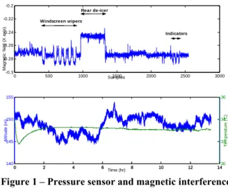
The pressure sensor measurements are affected by this kind of error as well, but they are also dependent on atmospheric changes. In the bottom of Figure 1 is plotted data recorded during a whole night in a closed room. As it is shown, the altitude provided by the sensor varies from 145 meters up to 155 meters, whilst the temperature stays constant.
0 500 1000 1500 2000 2500 3000 -0.3 -0.28 -0.26 -0.24 -0.22 -0.2 Samples M a g n e ti c f ie ld ( X a x is ) 0 2 4 6 8 10 12 14 140 145 150 155 A lt it u d e ( m ) 0 2 4 6 8 10 12 1430 32 34 36 T e m p e ra tu re ( °C ) Time (hr) Windscreen wipers Rear de-icer Indicators
Figure 1 – Pressure sensor and magnetic interference issues.
The magnetometer’s model follows those of equation (1) and equation (2), but must be augmented to take into account random interferences that may occur while driving. The upper part of Figure 1 gives an
example of such perturbations caused by windscreen wipers, indicators or rear de-icer and affecting the IMU placed on the dashboard of a car.
The sensors assembly, whose components have been described above, is used as the inertial reference system of the integrated land vehicle navigation system. Gyrometers are used to compute the attitude of the IMU, whereas accelerometers and magnetometers compensate for the drifts, even when the vehicle is moving [5].
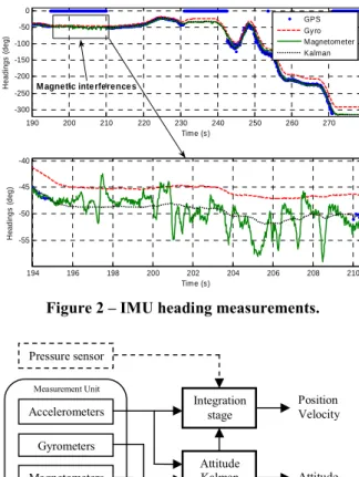
Figure 2 presents the headings computed with different algorithms during a trial in the city center. The upper part shows the drift of the gyro-based heading with respect to the magnetometer-based one. The GPS derived heading is plotted as well to assess the accuracy of the magnetic heading. The lower part focuses on magnetic interference mitigation. As expected, interferences occurred during the test conducted in the city centre. In the zoom presented Figure 2, the interference lasts about 15 seconds making the magnetic-derived heading unreliable. However, the Kalman filter that fuses the gyro and magnetometer measurements provides good estimate of true heading. The mitigation succeeds so that the attitude computed by the IMU can be used for navigation.
190 200 210 220 230 240 250 260 270 -300 -250 -200 -150 -100 -50 0 H e a d in g s ( d e g ) Time (s) 194 196 198 200 202 204 206 208 210 -55 -50 -45 -40 H e a d in g s ( d e g ) Time (s) GPS Gyro Magnetometer Kalman
M agnetic inte rfe rence s
Figure 2 – IMU heading measurements.
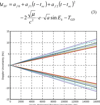
Figure 3 – Inertial Measurement Unit Mechanization. The pressure sensor is the last component of the
sensors assembly. It is used to check the vertical velocity as well as the vertical position. Figure 3 summarizes the inertial navigation mechanization.
II – GPS MEASUREMENT UNIT
The GPS measurement unit used in this study is composed of two parts. The first one is the receiver itself, whereas the second one is the assistance data.
a) Receiver core
The first part of the GPS measurement unit is a conventional receiver able to acquire and track signals down to 30 dBHz. It is also capable of providing measurements from the different tracking loops as well as pseudoranges with a sampling frequency up to 20 Hz. In our application, only Doppler and pseudorange measurements will be used in the integrated navigation system.
b) Assistance data
The second part of the GPS measurement unit is composed of the assistance data. They are threefold: satellites’ ephemeris augmented with ionospheric delay coefficients, rough user’s position and rough GPS time.
Ephemeredes and ionospheric delay coefficients are collected using a master GPS receiver operating under clear sky conditions. These data do not help the GPS receiver core to improve the signal acquisition performance.
Rough user’s position and GPS time are provided only when the GPS unit is started and has not yet given any measurements. This corresponds to the so-called “cold-start” mode. Once the first measurements are available and the initial position has been computed by the receiver, they are no more used as assistance data. The user’s position needed to process the ephemeris data is then given whether by the Integrated Navigation System (INS) or the IMU.
The combination of GPS measurements with assistance data allows the computation of four parameters that are useful for the Integrated Navigation System. The first one is the predicted satellite’s Doppler contribution, which is computed using ephemeris data, user’s position and GPS time. This contribution is estimated with some uncertainty since both position and time are known approximately, at least in the “cold-start” mode.
Given this worst case, an example of the error made on the estimation of the satellites’ Doppler contributions is plotted in Figure 4. This simulation
Attitude Kalman Filter Accelerometers Gyrometers Measurement Unit Magnetometers Low-cost MEMS sensors
Integration stage Position Velocity Attitude Pressure sensor
involves 11 ephemeredes recorded from visible satellites, but does not take into account time uncertainty, which may introduce extra +/-2 Hz error.
The satellite clock correction model is as described in [1]. The receiver core is capable of tracking GPS signals on both L1 and L2, but in our study only the
L1 acquisition and tracking is used. As a consequence,
using the notations of [1], the Space Vehicle clock correction model is as follows:
(
)
(
)
GD k oc f oc f f SVT
E
a
e
c
t
t
a
t
t
a
a
t
−
⋅
⋅
−
−
+
−
+
=
∆
sin
2
2 2 2 1 0µ
(3) 0 2000 4000 6000 8000 10000 12000 14000 16000 -15 -10 -5 0 5 10 15User's Horizontal Position Uncertainty (m)
D o p p le r U n c e rt a in ty ( H z )
Figure 4 – Satellite Doppler Uncertainty. Assistance data are also used to estimate the
tropospheric delay affecting the pseudorange
measurements. In this paper, the classical Hopfield model given in equation (6) is used.
(
)
amb amb amb d P T T K ⋅ + ⋅ + ⋅ ⋅ = − 16 , 273 72 , 148 40136 10 55208 , 1 4 (4)(
)
vap amb amb w P T T K ⋅ + + + ⋅ − = 16 , 273 2 , 8307 16 , 273 282 , 0 (5)(
)
(
2 3)
3 210
6854
,
0
sin
10
904
,
1
sin
− −⋅
+
+
⋅
+
=
∆
E
K
E
K
T
w d (6) where :–
T
amb is the standard ambient air temperature. –P
amb is the standard ambient pressure. –E
is the elevation of the satellite (unit : rad).–
P
vap is the standard ambient vapour pressure. –∆
T
is the tropospheric delay (unit : m).In the following, standard conditions will be taken into account, except the ambient pressure that will be provided by the pressure sensor. Consequently, Tamb=288,16K, Pvap=8,5hPa and Pamb=PMS5534.
The last information provided by the processing of the assistance data is the ionospheric delay impacting the L1 pseudorange measurements. Despite the
dual-frequency capabilities of the receiver core, the Klobuchar algorithm is used for ionospheric delay estimation.
Finally, the GPS Measurement Unit used in this study is composed of a single frequency (L1) receiver core
capable of providing Doppler and pseudorange
measurements. It is augmented with extra information such as satellite’s Doppler contribution and clock bias, ionospheric and tropospheric delays. The principle of the GPS Measurements Unit is summarized in Figure 5.
This unit is then integrated with the IMU described in section I, as discussed in the next section.
Figure 5 – GPS Measurement Unit.
III – INTEGRATED NAVIGATION SYSTEM Several integration schemes can be used to fuse GPS and IMU data. They all can be separated into three categories, namely loose coupling, tight coupling and ultra-tight coupling. Loose coupling is a very famous integration method that gives a great deal of performance for a minimal complexity. It uses GPS position and velocity measurements to correct the data from the IMU. Tight coupling goes deeper in the integration process since it uses raw GPS measurements (Doppler, pseudoranges, delta ranges…) to correct IMU errors. Ultra-tight coupling is the highest integration level, where IMU measurements are used to control GPS tracking
Rough position
Rough GPS time Ephemeredes & iono
Assistance data Acquisition Tracking loops Receiver Assistance data processing Pseudoranges Carrier Doppler Satellite Doppler Satellite clock correction Ionosphere correction Troposphere correction
INS/IMU Position
loops oscillator.
In this study, a tight coupling method is investigated to fuse GPS and IMU data and face urban navigation issues when very few GPS measurements are available. Raw pseudorange measurements are collected from the receiver for position correction. The processing of the ephemeredes provides ionospheric, tropospheric and satellite clock corrections so that corrected pseudoranges are fed in the Kalman filter. Because the vehicle is likely to go in urban / deep urban canyons, multi-path may affect these measurements and so the position solution. As a consequence, the receiver Doppler corrected for the satellite contribution is used as the second GPS measurement in the Kalman filter since it is more robust on such perturbations.
The IMU provides position and velocity, whose respective biases are estimated in the filter. Attitude measurements are processed separately to remove drift in pitch, roll and heading angles, as well as to reduce the impact of magnetic interferences on the filtered heading.
The Kalman filter used to fuse both navigation systems is composed of 8 states, as given in equation (7). The biases of the gyros are not estimated in the Kalman filter but their estimation is rather done in the attitude filter of the IMU.
r r V NED V NED
clk
clk
b
V
SF
P
AlongTrack∂
(7) where: − NEDP
is the vehicle position in the navigation frame. This includes North, East and Down components. −SF
V is the along track velocity scale factor.− NED
AlongTrack
V
is the true along track velocity in the navigation frame.−
b
V is the bias affecting velocity measurements. −clk
r is the receiver clock bias.−
∂
clk
r is the receiver clock drift.As discussed above, the measurements used in the filter are of three types and follow the relations given in (8), (9) and (10). V NED AlongTrack V IMU AlongTrack
SF
V
b
V
=
×
+
(8)(
AT LOS)
NED AlongTrack LO d receiver GPS corrected df
g
V
f
,=
+
,
α
/ (9) r receiver GPS corrected=
∆
N
+
∆
E
+
∆
D
+
c
⋅
clk
2 2 2ρ
(10) where: − receiver correctedρ
is the pseudorange corrected for theionosphere, troposphere and satellite clock biases.
− receiver
corrected d
f
, is the Doppler frequency corrected for thesatellite contribution.
−
α
AT/LOS is the Along Track to Line Of Sight projection coefficient.−
g
is a non-linear function that computes the user’sDoppler contribution using NED
AlongTrack
V
andα
AT/LOS asparameters.
−
c
is the velocity of light −L
1 is the GPS L1 frequency.−
∆
N
is the north position difference between the vehicle and the satellite at time of transmission. −∆
E
is the east position difference between thevehicle and the satellite at time of transmission. −
∆
D
is the down position difference between thevehicle and the satellite at time of transmission. The projection coefficient
α
AT/LOS that must be applied to the true velocity along the track followed by the vehicle is computed using the satellite position at time of transmission, the position of the vehicle and the result of the processing of the data provided by the IMU.The integrated navigation system principle is summarized in Figure 6. Five measurements at most are fused in the Kalman filter to provide a position solution and also augment the system availability.
Figure 6 – Integrated Navigation System.
Kalman
Filter
Attitude measurements Velocity measurementsInertial Measurement Unit
Position Doppler measurements Pseudorange measurements GPS Measurement Unit Velocity
This navigation system is then tested in actual urban conditions. Results are given in the next section.
IV – TEST RESULTS
This section presents the results of the tests conducted with the system described above. The capability of the INS to provide a position solution in challenging urban canyon conditions is more specifically addressed. The focus is put on the navigation using the IMU and the measurements of only two GPS satellites. IMU data are recorded at 25Hz, whereas GPS data are recorded at 1Hz.
The reference trajectory is plotted in Figure 7 as the red path. The traveled distance in the exercised vehicle trial is about 4,5 km for 15 minutes of navigation in urban conditions. The position solution given by the OEM4 GPS receiver is also plotted in blue, and corresponding statistics are given in Table 2.
OEM4 Tracking status. Nb of
satellites 0 – 1 2 3 ≥ 4
% of
time 7,2% 12,3% 14% 66,5%
Table 2 – OEM4 tracking performance. As it can be seen in Figure 7, the position solution availability is medium (66,5 %), that does not allow a full urban navigation. The receiver tracked at least 2 satellites about 93% of the time, which makes the trial suitable for testing the proposed tight integration. During the trial, GPS measurements experienced large errors certainly due to multi-path, as shown by the position solutions inside the green circles.
Figure 7 – Reference trajectory & OEM4 trajectory.
In the following, the two latest satellites that are acquired and tracked will be used in the Integrated Navigation System in order to process data from many satellite configurations and thus simulate real conditions where only 2 GPS measurements were available. In the exercised trial, the satellite configuration, that is the combination of two GPS measurements, changes approximately every 8 seconds.
As a comparison of both navigation systems intrinsic performance, the trajectory computed exclusively with the data provided by the IMU is plotted in Figure 8. In this test, the heading was initialized using the magnetometers and checked by the first GPS measurements.
Figure 8 – IMU based trajectories.
The magnetometers have been calibrated before the trial, so that the magnetic heading is not affected by interference due to the vehicle itself. Two trajectories have been computed, one using the gyro-derived heading (the green plot), the other using the filtered-derived heading (the red plot). As it can be seen in the figure, both trajectories are rapidly drifting. This is mainly due to the accelerometer bias that changes during the trial and impacts the velocity and position computation. The trajectory using the filtered heading provides however the best position solution.
In order to test first the ability of the INS to provide a reliable position solution using very few GPS measurements and second the accuracy of the heading provided by the IMU, a first hybridization is performed using only two Doppler measurements. Results are given in Figure 9. The trajectory using the gyro-derived heading is still unreliable. The gyro drifts affect obviously the heading but also the estimation of the along track velocity through equation (9).
Opposite, the position solution using the filtered heading is far more accurate. The trajectory shape is clearly recognizable and follows the true path quite well, with a horizontal error bounded by 100m for 15 minutes of navigation. The heading provided by the IMU is thus quite accurate, even if it is not perfect. Because the INS provides a position solution in a Dead Reckoning mode by integrating the debiased velocity, error accumulates so that the position is still drifting and will lead to an unreliable long term position solution. Both trajectories are not affected by multipath, as the GPS-based position is. This is mainly due to the fact that Doppler measurements are less sensitive to multipath than pseudoranges.
Figure 9 – INS trajectories. 2 Doppler measurements used when available.
The above hybridization shows that the use of only Doppler measurements does not allowed the computation of a reliable position with an error bounded in time. As a consequence, pseudorange measurements seem necessary in the integration process.
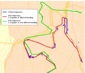
Another hybridization is therefore performed using only two Doppler and two pseudorange measurements. The filtered attitude provided by the IMU is used in this test. The resulting trajectory provided by the INS is plotted in Figure 10 in red. As a comparison, the GPS trajectory is also plotted in blue.
It can obviously be noticed that the overall accuracy is tremendously improved with the use of pseudorange measurements. The horizontal error stays indeed within 40 meters from the reference trajectory. Even if pseudoranges are used, the hybridized INS trajectory is again resistant to multipath affecting the GPS measurements because of the high confidence in the
Doppler measurement model and the position
computation strategy implemented in the Kalman filter.
Figure 10 – INS trajectory. 2 Doppler and 2 pseudorange measurements used when available.
In this hybridization test, position estimations with and without height-aiding were performed. However, the horizontal position solution does not vary very much from each integration scheme that is why only the non height-aided solution is plotted in Figure 10.
Figure 11 shows the vertical performance of the hybridized system using only two Doppler and two pseudorange measurements. The upper part of the figure gives the vertical accuracy, with respect to the pressure sensor measurements. As it can be seen in the figure, the vertical error reaches about 30 meters without height-aiding, whereas it stays below 5 meters when the altitude is used in the Kalman filter.
0 100 200 300 400 500 600 700 800 900 0 10 20 30 (m ) KF Height error 100 200 300 400 500 600 700 800 900 160 162 164 166 168 Time (s) A lt it u d e ( m ) Pressure Sensor W ithout Height aiding
W ith Height aiding
Figure 11 – INS vertical error. 2 Doppler and 2 pseudorange measurements used when available.
However, the path followed during the test was quite flat, as shown in the lower part of the figure. Thus, the capability of the filter to bound the vertical error when
height-aiding is performed has to be considered with care. The vertical accuracy should be assessed with a hilly path. The velocity profile of the vehicle computed using two Doppler and two pseudorange measurements is plotted in Figure 12. The velocity of the INS is well debiased compared to the one provided by the IMU itself and that is fed in the Kalman filter. However, the along track velocity profile experiences sudden variations that affect the position solution. Some may be very large, as shown by the black circles in Figure 10.
0 0.5 1 1.5 2 2.5 3 3.5 4 4.5 x 10⁴ -180 -160 -140 -120 -100 -80 -60 -40 -20 0 20 Samples V e lo c it y ( m /s ) INS velocity IMU velocity
Figure 12 – Along track velocity profile. Two velocity profile zooms are plotted in Figure 13 to clearly observe the discontinuities that sometimes appear. 3.87 3.88 3.89 3.9 3.91 3.92 3.93 3.94 3.95 3.96 3.97 x 10⁴ 5 10 15 Samples V e lo c it y ( m /s ) 6500 6550 6600 6650 6700 6750 6800 6850 6900 6950 5 6 7 8 Samples V e lo c it y ( m /s )
Figure 13 – Velocity profile discontinuities. In these two examples, discontinuities clearly occur around samples 6750 and 39600. They can be due to two events. The first one occurs when the hybridized solution relies exclusively on IMU data, thus accumulates errors, and then is corrected by GPS data. The second one occurs when low quality GPS data are used to correct the
velocity and the position provided by the IMU. Since in our case, discontinuities appear when GPS measurements are combined with IMU data, the hybridization methodology can be considered responsible for those issues.
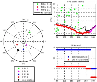
Figure 14 presents three different plots that explain the reasons of this bad velocity estimation when GPS and IMU data are tightly integrated. The lower right plot gives the PRNs used in the Kalman filter, the upper right plot the velocity computed using these different PRNs and the left plot the satellite geometry and user heading at time of data combination. At the beginning, PRN 14 and 6 are used for hybridization. Based on these two PRNs, the user’s velocity along the track followed by the vehicle has been computed and plotted. It corresponds to the green dots in the upper right plot. As it can be stated, this velocity has got a large variance.
1 2 30 210 60 240 90 270 120 300 150 330 180 0 PRN 5 PRN 1 PRN 14 PRN 6 user heading 50 100 150 200 250 300 4 5 6 7 8 9 10 11 (m /s ) GPS-based velocity PRNs 6-14 PRNs 5-14 PRNs 5-1 KF velocity 50 100 150 200 250 300 0 5 10 15 PRNs used 1st measurement 2nd measurement
Figure 14 – Satellite geometry issue.
The position of PRN 14 when it is used in the Kalman filter is plotted on the left as the blue dots, whereas the position of PRN 6 is plotted as the red dots. The heading of the user is also referenced as the black dots. Obviously, given this satellites configuration with respect to the user’s heading, the estimation of the user’s Doppler contribution is very difficult, even not possible. This explains why the GPS-based user’s velocity is very noisy.
The Kalman filter uses then PRNs 14 and 5 to estimate the along track velocity. The configuration of the satellite’s position with respect to the user’s heading is far better, as it can be seen in the left plot. This also explains why the user’s velocity is computed with much accuracy, as shown with the red curve in the upper right plot. It can thus be stated that the satellite geometry is of tremendous importance to estimate the velocity of the vehicle, as the DOP is for GPS positioning accuracy.
To avoid this discontinuity issue, a criterion based on the geometry of the satellites used for hybridization has been implemented. When bad configurations are detected, GPS measurements are no more taken into account, but the INS relies exclusively on the IMU data.
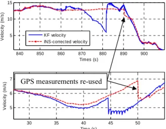
The results of the along track velocity estimation is plotted in Figure 15, using only two Doppler measurements to avoid the pseudoranges to interfere in the velocity and position computation. The improvement is not obvious. It could either perform better or worse. Sudden variations are still observable, but in that case, they are due to the re-use of new good GPS measurements. The performance of the INS without GPS updates depends directly on the quality of the sensors that are used. 840 850 860 870 880 890 900 5 10 15 Times (s) V e lo c it y ( m /s ) 30 35 40 45 50 5 6 7 Time (s) V e lo c it y ( m /s ) KF velocity INS-corrected velocity KF velocity INS-corrected velocity
Figure 15 – Velocity profile corrected by IMU measurements when bad satellites configurations are
detected.
Figure 16 – Corrected and non-corrected INS trajectories.
The improvement on the position solution is not obvious as well, as it can be noticed in Figure 16. Even if the horizontal accuracy stays within 100 meters from the reference trajectory, the final error is worst than without IMU-based corrections.
CONCLUSION
This paper investigated the land vehicle navigation using low-cost sensors and a conventional GPS receiver using very few GPS measurements for the tight hybridization. It as been shown that two Doppler and two pseudorange measurements were sufficient to allow the estimation of the bias affecting the velocity provided by a low-cost MEMS-based IMU.
The use of only two Doppler measurements shows that the accuracy of the heading provided by the IMU was reliable enough to provide a good short term position solution. Long term positioning is rather difficult since the trajectory is slowly drifting because residual biases affect the attitude of the IMU. However, a horizontal error within 100m is achievable for 15 min of navigation with only two Doppler measurements.
The adjunction of two pseudorange
measurements tremendously improves the position accuracy. A horizontal error within 40 meters of the reference trajectory can indeed be achieved using only two Doppler and two pseudorange measurements. No more drift is noticeable in the Integrated Navigation System position solution.
Height aiding improves the vertical accuracy that is reduced from 30 meters to 5 meters with the adjunction of pressure sensor measurements in the Kalman filter. The trial exercised here was quite flat, so hilly tests should be performed to assess this improvement.
However, the Integrated Navigation System is dependent on the geometry of the satellites used for hybridization, especially when only two measurements are used. Bad satellites configurations with respect to the user’s heading yield to erroneous velocity updates. A detection criterion has thus been implemented to prevent these configurations from biasing both the velocity and the position of the vehicle. During these periods, the performance of the Integrated Navigation System relies then exclusively on the quality of the sensors used in the IMU.
ACKNOWLEDMENTS
The authors would like to thank GeoConcept for the GIS software used in the study.
REFERENCES
[1] – Global Positioning System Standard Positioning Service Signal Specification, 2nd edition, June 1995.
[2] – S. Godha et al., Performance Analysis of MEMS / IMU / HSGPS / Magnetic Sensor Integrated System in Urban Canyons, ION GNSS 2005.
[3] – S. Godha and M. E. Cannon, Integration of DGPS with a Low Cost MEMS – Based Inertial Measurement Unit (IMU) for Land Vehicle Navigation Application, ION GNSS 2005.
[4] – Collin J., J. Kappi, and K. Saarinen, Unaided
MEMS-Based INS Application in a Vehicular
Environment, ION GNSS 2001.
[5] – Kubrak D., Macabiau C. and Monnerat M., Performance Analysis of MEMS based Pedestrian Navigation Systems, ION GNSS 2005.
[6] – Intersema MS5534 data sheet.
[7] – Analog Devices ADXL202E data sheet. [8] – Analog Devices ADXRS300 data sheet. [9] – Philips KMZ52 data sheet.