HAL Id: hal-00879347
https://hal.archives-ouvertes.fr/hal-00879347
Submitted on 6 Jan 2016
HAL is a multi-disciplinary open access
archive for the deposit and dissemination of
sci-entific research documents, whether they are
pub-lished or not. The documents may come from
teaching and research institutions in France or
abroad, or from public or private research centers.
L’archive ouverte pluridisciplinaire HAL, est
destinée au dépôt et à la diffusion de documents
scientifiques de niveau recherche, publiés ou non,
émanant des établissements d’enseignement et de
recherche français ou étrangers, des laboratoires
publics ou privés.
and occultation measurements
Viktoria F. Sofieva, N. Rahpoe, J. Tamminen, E. Kyrölä, N. Kalakoski, M.
Weber, A. Rozanov, C. von Savigny, A. Laeng, T. von Clarmann, et al.
To cite this version:
Viktoria F. Sofieva, N. Rahpoe, J. Tamminen, E. Kyrölä, N. Kalakoski, et al.. Harmonized dataset
of ozone profiles from satellite limb and occultation measurements. Earth System Science Data,
Copernicus Publications, 2013, 5 (2), pp.349-363. �10.5194/essd-5-349-2013�. �hal-00879347�
www.earth-syst-sci-data.net/5/349/2013/ doi:10.5194/essd-5-349-2013
©Author(s) 2013. CC Attribution 3.0 License. Open
Access
Science
Data
Harmonized dataset of ozone profiles from satellite limb
and occultation measurements
V. F. Sofieva1, N. Rahpoe2, J. Tamminen1, E. Kyrölä1, N. Kalakoski1, M. Weber2, A. Rozanov2,
C. von Savigny3, A. Laeng4, T. von Clarmann4, G. Stiller4, S. Lossow4, D. Degenstein5, A. Bourassa5,
C. Adams5, C. Roth5, N. Lloyd5, P. Bernath6,7, R. J. Hargreaves6, J. Urban8, D. Murtagh8,
A. Hauchecorne9, F. Dalaudier9, M. van Roozendael10, N. Kalb10, and C. Zehner11 1Finnish Meteorological Institute, Helsinki, Finland
2Institute of Environmental Physics, University of Bremen, Bremen, Germany 3Institute of Physics, University of Greifswald, Greifswald, Germany
4Karlsruhe Institute of Technology, Institute for Meteorology and Climate Research, Germany 5Institute for Space and Atmospheric Studies, University of Saskatchewan, Saskatoon, Saskatchewan, Canada
6Department of Chemistry, University of York, York, UK
7Department of Chemistry & Biochemistry, Old Dominion University, Norfolk, VA, USA
8Chalmers University of Technology, Department of Earth and Space Sciences, 41296 Gothenburg, Sweden 9Université Versailles St-Quentin, UPMC University Paris 06, CNRS/INSU, LATMOS-IPSL,
78280 Guyancourt, France
10Belgian Institute for Space Aeronomy (IASB-BIRA), Brussels, Belgium 11ESA/ESRIN, Frascati, Italy
Correspondence to: V. F. Sofieva ([email protected])
Received: 30 May 2013 – Published in Earth Syst. Sci. Data Discuss.: 14 June 2013 Revised: 3 October 2013 – Accepted: 9 November 2013 – Published: 2 December 2013
Abstract. In this paper, we present a HARMonized dataset of OZone profiles (HARMOZ) based on limb and occultation measurements from Envisat (GOMOS, MIPAS and SCIAMACHY), Odin (OSIRIS, SMR) and SCISAT (ACE-FTS) satellite instruments. These measurements provide high-vertical-resolution ozone profiles covering the altitude range from the upper troposphere up to the mesosphere in years 2001–2012. HARMOZ has been created in the framework of the European Space Agency Climate Change Initiative project.
The harmonized dataset consists of original retrieved ozone profiles from each instrument, which are screened for invalid data by the instrument teams. While the original ozone profiles are presented in di ffer-ent units and on different vertical grids, the harmonized dataset is given on a common pressure grid in netCDF (network common data form)-4 format. The pressure grid corresponds to vertical sampling of ∼ 1 km below 20 km and 2–3 km above 20 km. The vertical range of the ozone profiles is specific for each instrument, thus all information contained in the original data is preserved. Provided altitude and temperature profiles allow the representation of ozone profiles in number density or mixing ratio on a pressure or altitude vertical grid. Geolocation, uncertainty estimates and vertical resolution are provided for each profile. For each instrument, optional parameters, which are related to the data quality, are also included.
For convenience of users, tables of biases between each pair of instruments for each month, as well as bias uncertainties, are provided. These tables characterize the data consistency and can be used in various bias and drift analyses, which are needed, for instance, for combining several datasets to obtain a long-term climate dataset.
This user-friendly dataset can be interesting and useful for various analyses and applications, such as data merging, data validation, assimilation and scientific research.
The dataset is available at http://www.esa-ozone-cci.org/?q=node/161 or at doi:10.5270/esa-ozone_cci-limb_occultation_profiles-2001_2012-v_1-201308.
1 Introduction
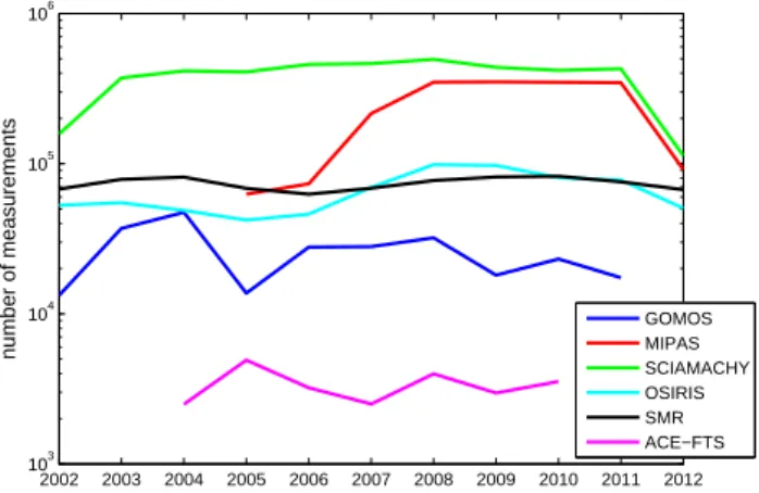
The creation of homogenized ozone profile datasets based on limb or occultation measurements from sensors on board the European Space Agency (ESA) Envisat satellite, as well as from ESA Third Party Missions (TPM), is one of the primary objectives of the European Space Agency Climate Change Initiative project (Ozone_cci, http://www. esa-ozone-cci.org). Six instruments that provide long-term measurements are involved in this project. Three of them are on board Envisat: Global Ozone Monitoring by Occultation of Stars (GOMOS), Michelson Interferometer for Passive At-mospheric Sounding (MIPAS) and Scanning Imaging Spec-trometer for Atmospheric Chartography (SCIAMACHY); two of them are on board Odin: Optical Spectrograph and InfraRed Imaging System (OSIRIS) and Sub-Millimeter Ra-diometer (SMR), and one is on board the SCISAT-1 satel-lite: Atmospheric Chemistry Experiment – Fourier Trans-form Spectrometer (ACE-FTS). Three of the instruments – GOMOS, SCIAMACHY and OSIRIS – retrieve ozone profiles from measurements in the UV–visible wavelength range. MIPAS and ACE-FTS use infrared wavelengths, and SMR operates at sub-millimeter wavelengths. Two of the in-struments use the occultation technique: GOMOS uses stel-lar occultation and ACE-FTS performs sostel-lar occultations. SCIAMACHY and OSIRIS are limb-scattering instruments; MIPAS and SMR measure thermal emission spectra. More details on individual datasets are presented in Sect. 3. Over-all, the datasets cover the years 2001–2012 (not all instru-ments cover the whole time period). The yearly data vol-ume for the HARMOZ instrvol-uments is illustrated in Fig. 1. Between the various datasets, there are ozone measurements available for all seasons, various times of day, and good lati-tudinal coverage (as an example, Fig. 2 illustrates the latitu-dinal coverage in 2008).
The data from different sensors have different proper-ties such as specific quality flags, and the data can have outliers due to problematic retrievals under some condi-tions. In some cases (like for GOMOS), ozone data qual-ity strongly depends on a set of parameters, which makes using this dataset complicated for non-experts. As a first step towards data homogenization, we have created a HAR-Monized dataset of OZone profiles (HARMOZ). HARMOZ consists of independent datasets from individual instruments, which are carefully screened for outliers, interpolated to a common pressure grid and saved in the common netCDF (network common data form)-4 format. This database is used in various “higher-level” analyses performed within the Ozone_cci project (in particular, in creating Level 3 data, see the Ozone_cci web page http://www.esa-ozone-cci.org/ ?q=node/160 for details). Convenience of using the harmo-nized dataset has prompted us to make this dataset avail-able to the scientific community. This dataset contributes to the initiative on past changes in the vertical distribution of ozone (SI2N (SPARC – Stratospheric Processes and their
2002 2003 2004 2005 2006 2007 2008 2009 2010 2011 2012 103 104 105 106 number of measurements GOMOS MIPAS SCIAMACHY OSIRIS SMR ACE−FTS
Figure 1.Number of measurements in each year and for each in-strument. Number of MIPAS and SCIAMACHY measurements de-crease significantly in 2012 due to the loss of Envisat. GOMOS data from year 2012 are not included in HARMOZ, because GOMOS experienced instrumental problems at that time.
Role in Climate, IO3C – International Ozone Commission,
IGACO-O3– Integrated Global Atmospheric Chemistry
Ob-servations, NDACC – Network for the Detection of Atmo-spheric Composition Change) initiative, http://igaco-o3.fmi. fi/VDO/working_groups.html).
The paper is organized as follows. Section 2 presents a general description of the dataset and the data processing. Each dataset has mandatory parameters, which are the same for all instruments (discussed in Sect. 2), as well as optional, instrument-specific parameters (discussed in Sect. 3). The data format and availability are presented in Sect. 4. To char-acterize the data consistency, tables of biases between each pair of instruments are created. The construction and format of the bias tables are discussed in Sect. 5. The summary con-cludes the paper.
2 General description of the harmonized dataset
The individual datasets from each instrument passed qual-ity control, which has been performed by the instrument ex-perts. The quality control procedures are described in detail in Sect. 3. Only valid data are included in HARMOZ.
Each profile has been interpolated onto a common pres-sure grid (Ozone_cci prespres-sure grid hereafter), which is an extension of the SPARC Data Initiative pressure grid (Heg-glin and Tegtmeier, 2010; Tegtmeier et al., 2013). The Ozone_cci pressure levels and the corresponding pressure al-titudes are presented in Appendix A. The vertical spacing of the Ozone_cci grid corresponds to ∼ 1 km below 20 km and
∼ 2–3 km above. The number of pressure levels included in
the individual datasets depends on the valid altitude range of the ozone profiles. For example, GOMOS data are pro-vided on the Ozone_cci grid in the range 250–10−4hPa,
while MIPAS data are provided in the range 400–0.05 hPa.
1 2 3 4 5 6 7 8 9 10 11 12 −80 −60 −40 −20 0 20 40 60 80 latitude GOMOS 1 2 3 4 5 6 7 8 9 10 11 12 −80 −60 −40 −20 0 20 40 60 80 MIPAS 1 2 3 4 5 6 7 8 9 10 11 12 −80 −60 −40 −20 0 20 40 60 80 SCIAMACHY 1 2 3 4 5 6 7 8 9 10 11 12 −80 −60 −40 −20 0 20 40 60 80 month latitude OSIRIS 1 2 3 4 5 6 7 8 9 10 11 12 −80 −60 −40 −20 0 20 40 60 80 month SMR 1 2 3 4 5 6 7 8 9 10 11 12 −80 −60 −40 −20 0 20 40 60 80 month ACE 0 0.5 1 1.5 2 2.5 3 3.5 4 log 10 (number of measurements)
Figure 2.Logarithm of number of measurements in 10◦latitude zones and in each month of year 2008.
28
Figure 2. Logarithm of number of measurements in 10
latitude zones and in each
month of year 2008.
Figure 3 Illustration of altitude ranges of ozone measurements for the individual
in-struments in HARMOZ. The vertical axis is not to scale.
Vertical grid and altitude range
•
Extended SPARC-DI grid
•
All CCMVal levels are
included
•
Vertical spacing
~ 1 km below 20 km
~2-3 km above 20 km
•
Altitude range is
instrument-dependent
•
Altitude profiles are also
provided
GO
MOS
ACE
-F
T
S
OS
IRI
S
SCIAMACHY
MIP
A
S
SMR
Pr es sure , hPa alti tud e, km 10-4 112 210-4 107 0.05 70 65 0.1 10 6.5 5.6 450 400 250 300 8.5Figure 3.Illustration of altitude ranges of ozone measurements for the individual instruments in HARMOZ. The vertical axis is not to scale.
The altitude range of the individual datasets can be found in Table 1 and is illustrated in Fig. 3. The largest altitude range is achieved for occultation instruments, which cover also the lower thermosphere.
The data files contain the mandatory variables that are the same for all sensors. The main variables are profiles of ozone concentrations (moles cm−3) and their uncertain-ties. The auxiliary information includes temperature and al-titude profiles at the measurement locations for converting ozone data to different units (mixing ratio/number density on pressure/altitude in all possible combinations), as well as geolocation, time, and vertical resolution. The full list of mandatory parameters is presented in Table 2. The optional, instrument-specific parameters, which include those related to the quality of data, can be found in Table 3; they are discussed in more detail in Sect. 3. The data are written in the netCDF-4 format, in agreement with standard conven-tions (http://cf-pcmdi.llnl.gov/documents/cf-conventions/1. 6). Each netCDF file (for each instrument) contains the data from one month (see Sect. 5 for more details on data format). For regridding of profiles, a linear interpolation in the logarithm-pressure vertical coordinate is used. The altitude-pressure profiles needed for the interpolation are based on retrieved data or taken from the meteorological model data
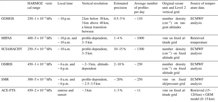
Table 1.General information about the datasets. Note that the average number of profiles per day is estimated from the average yearly volume, thus the number of profiles in each particular day can differ significantly from these average estimates.
HARMOZ verti-cal range
Local time Vertical resolution Estimated
precision
Average number of profiles per day
Original ozone unit and Level 2 vertical grid
Source of temper-ature data
GOMOS 250–1 × 10⁻⁴hPa ∼ 10 p.m. 2 km below 30 km,
3 km above 40 km, a linear transition between 0.5–5 % ∼ 110 number density (cm−3) on tan-gent altitudes ECMWF analysis
MIPAS 400–5 × 10⁻²hPa ∼ 10 p.m. and
∼ 10 a.m. profile-dependent, 3–5 km 1–4 % ∼ 1000 vmr on fixed al-titude grid Retrieved temperature
SCIAMACHY 250–5 × 10⁻²hPa ∼ 10 a.m. profile-dependent,
3–5 km 10–15 % ∼ 1300 number density (cm−3) on fixed altitude grid ECMWF analysis
OSIRIS 450–1 × 10⁻¹hPa ∼ 6 a.m. and
∼ 6 p.m. ∼ 2–3 km, altitude-dependent 2–10 % ∼ 250 number density (cm−3) on fixed altitude grid ECMWF analysis
SMR 300–5 × 10⁻²hPa ∼ 6 a.m. and
∼ 6 p.m.
profile-dependent, ∼ 2.5–3.5 km
∼ 20% ∼ 250 vmr on fixed
alt/pressure grid
ECMWF analysis
ACE-FTS 450–2 × 10⁻⁴hPa sunrise and
sunset ∼ 3 km 1–3 % ∼ 11 vmr on fixed al-titude grid Retrieved (15– 120 km)+ GEM model (0–15 km)
Table 2.Mandatory parameters in the HARMOZ netCDF files. Naltand Nprofdenote the number of pressure levels and the number of profiles, respectively.
Parameter and unit Dimensions Description
time (days since 1900-01-01 00:00:00)
Nprof× 1 The parameter to index the profiles
air_pressure (hPa) Nalt× 1 The vertical coordinate
altitude (km) Nalt× Nprof The geometric altitude above the mean sea-level latitude (deg north) Nprof× 1 Latitude of each profile (given at altitude ∼ 35 km) longitude (deg east) Nprof× 1 Longitude of each profile (given at altitude ∼ 35 km) mole_concentration_of_ozone
_in_air (moles cm−3)
Nalt× Nprof Vertical profiles of ozone. Number density (cm−3) is acquired by multiplying the variable with Avogadro constant NA= 6.02214 × 10²³moles−1
mole_concentration_of_ozone_in_air standard_error (moles cm−3)
Nalt× Nprof Uncertainty (random error) associated with the ozone profiles
vertical_resolution (km) Nalt× Nprofor Nalt× 1 FWHM of the averaging kernel
air_temperature (K) Nalt× Nprof Temperature profiles at the locations of measurements, for conversion from concentration to mixing ratio
(mainly, European Centre for Medium-Range Weather Fore-casts, ECMWF) at the locations of measurements (Table 1). This interpolation does not introduce significant inaccuracy, because the uncertainty of the altitude-pressure profiles is very small. For the instruments providing reliable covariance matrices of retrieval errors, the covariance matrices of
uncer-tainties (random error) were interpolated as
C= WCorigWT, (1)
where Corigand C are original and interpolated matrices,
re-spectively, and W is the interpolation matrix. The parameter “standard_error” contains the square roots of the diagonal el-ements of C; it represents the uncertainty (random error) of
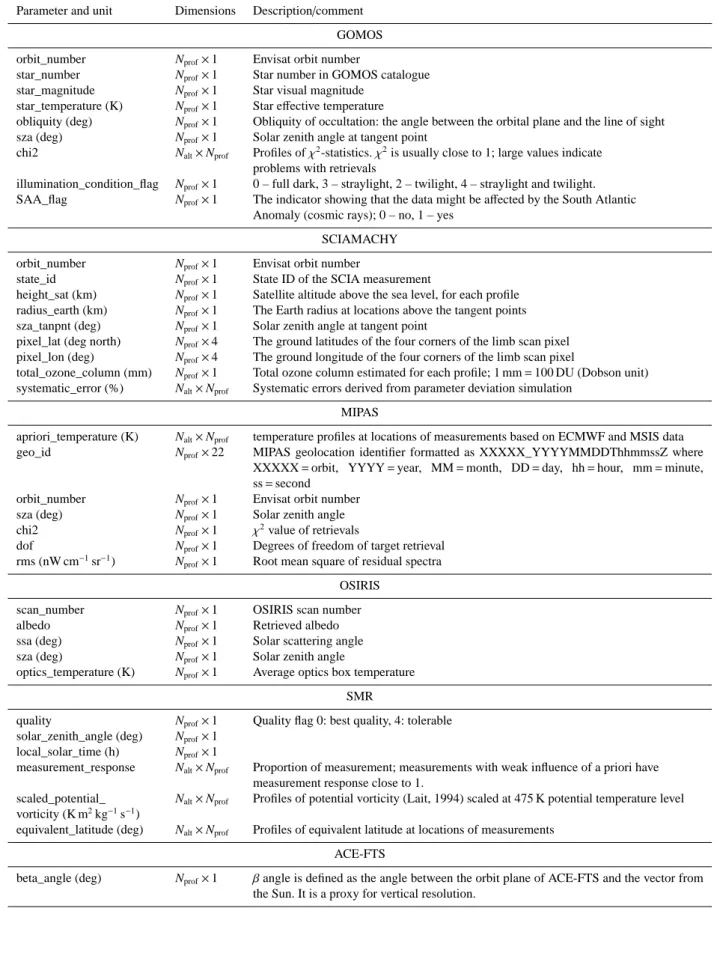
Table 3.Optional parameters in the HARMOZ netCDF files. Naltand Nprofdenote the number of pressure levels and the number of profiles, respectively.
Parameter and unit Dimensions Description/comment
GOMOS
orbit_number Nprof× 1 Envisat orbit number
star_number Nprof× 1 Star number in GOMOS catalogue
star_magnitude Nprof× 1 Star visual magnitude
star_temperature (K) Nprof× 1 Star effective temperature
obliquity (deg) Nprof× 1 Obliquity of occultation: the angle between the orbital plane and the line of sight
sza (deg) Nprof× 1 Solar zenith angle at tangent point
chi2 Nalt× Nprof Profiles of χ2-statistics. χ2is usually close to 1; large values indicate
problems with retrievals
illumination_condition_flag Nprof× 1 0 – full dark, 3 – straylight, 2 – twilight, 4 – straylight and twilight.
SAA_flag Nprof× 1 The indicator showing that the data might be affected by the South Atlantic
Anomaly (cosmic rays); 0 – no, 1 – yes SCIAMACHY
orbit_number Nprof× 1 Envisat orbit number
state_id Nprof× 1 State ID of the SCIA measurement
height_sat (km) Nprof× 1 Satellite altitude above the sea level, for each profile
radius_earth (km) Nprof× 1 The Earth radius at locations above the tangent points
sza_tanpnt (deg) Nprof× 1 Solar zenith angle at tangent point
pixel_lat (deg north) Nprof× 4 The ground latitudes of the four corners of the limb scan pixel
pixel_lon (deg) Nprof× 4 The ground longitude of the four corners of the limb scan pixel
total_ozone_column (mm) Nprof× 1 Total ozone column estimated for each profile; 1 mm= 100 DU (Dobson unit)
systematic_error (%) Nalt× Nprof Systematic errors derived from parameter deviation simulation
MIPAS
apriori_temperature (K) Nalt× Nprof temperature profiles at locations of measurements based on ECMWF and MSIS data
geo_id Nprof× 22 MIPAS geolocation identifier formatted as XXXXX_YYYYMMDDThhmmssZ where
XXXXX= orbit, YYYY = year, MM = month, DD = day, hh = hour, mm = minute,
ss= second
orbit_number Nprof× 1 Envisat orbit number
sza (deg) Nprof× 1 Solar zenith angle
chi2 Nprof× 1 χ2value of retrievals
dof Nprof× 1 Degrees of freedom of target retrieval
rms (nW cm−1sr−1) N
prof× 1 Root mean square of residual spectra
OSIRIS
scan_number Nprof× 1 OSIRIS scan number
albedo Nprof× 1 Retrieved albedo
ssa (deg) Nprof× 1 Solar scattering angle
sza (deg) Nprof× 1 Solar zenith angle
optics_temperature (K) Nprof× 1 Average optics box temperature
SMR
quality Nprof× 1 Quality flag 0: best quality, 4: tolerable
solar_zenith_angle (deg) Nprof× 1
local_solar_time (h) Nprof× 1
measurement_response Nalt× Nprof Proportion of measurement; measurements with weak influence of a priori have
measurement response close to 1. scaled_potential_
vorticity (K m2kg−1s−1)
Nalt× Nprof Profiles of potential vorticity (Lait, 1994) scaled at 475 K potential temperature level
equivalent_latitude (deg) Nalt× Nprof Profiles of equivalent latitude at locations of measurements
ACE-FTS
beta_angle (deg) Nprof× 1 β angle is defined as the angle between the orbit plane of ACE-FTS and the vector from
the Sun. It is a proxy for vertical resolution.
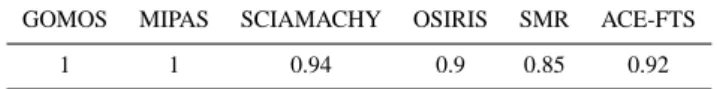
Table 4.The approximate reduction factors for uncertainty esti-mates due to regridding (the reported values of uncertainties should be multiplied with the factor from the table).
GOMOS MIPAS SCIAMACHY OSIRIS SMR ACE-FTS
1 1 0.94 0.9 0.85 0.92
individual profiles. Due to the structure of Corig and W,
di-agonal elements of C are very slightly reduced compared to the diagonal elements of Corig. For the instruments, for which
covariance matrices are not easily available or insufficiently reliable, the uncertainty estimates were simply linearly inter-polated to the Ozone_cci grid (in the same way as the ozone profiles). In these cases, the reduction of uncertainties due to interpolation has been estimated based on a sample co-variance matrix and the information about the vertical reso-lution and the original grid. This reduction is very small, of a factor ∼ 0.85–0.95 (Table 4). It should be stressed here that the correction factors presented in Table 4 approximate only changes in uncertainty estimates due to regridding.
Note also that the Ozone_cci grid is finer than the vertical resolution of the ozone profiles, therefore the uncertainties at adjacent layers are correlated. Without covariances provided, there is the risk to overestimate the independent information contained in the profiles. For some of the instruments, there exist “advanced” versions of HARMOZ files with full co-variance matrices C stored. These data can be provided upon request.
Three instruments (GOMOS, SCIAMACHY and OSIRIS) provide ozone number density profiles, thus the conver-sion to concentration (moles cm−3), the unit used in HAR-MOZ, is simply division by the Avogadro constant NA=
6.02214 × 10²³moles−1. MIPAS, ACE-FTS and SMR
re-trieve ozone mixing ratio profiles. For MIPAS and ACE-FTS, the retrieved temperature and pressure profiles were used for conversion to HARMOZ ozone concentration rep-resentation, thus making it fully consistent with the origi-nal mixing-ratio profiles. For SMR, temperature profiles are taken from the ECMWF fields. Therefore, small (∼ 0.1 %) drifts and jumps in the ECMWF density (which can be caused, for example, by different amounts of assimilated data over time, http://www.ecmwf.int/research/era/do/get/index/ QualityIssues) can induce an additional uncertainty of the same magnitude in SMR ozone concentrations reported in HARMOZ.
3 Short descriptions of individual datasets
In this section, a brief overview of the individual datasets is presented. The general parameters of the individual datasets are collected in Table 1. They include information about the altitude range of individual datasets, typical local time, ver-tical resolution, original representation of ozone profiles, as
well as the source of air density data, which can be used for conversion from ozone concentration to mixing ratio. Spe-cific features of individual datasets are described below.
3.1 GOMOS
GOMOS is a stellar occultation instrument on board Envisat (Bertaux et al., 2010; Kyrölä et al., 2010). Ozone profiles are retrieved from UV–visible spectrometer measurements at wavelengths 250–692 nm. In this dataset, nighttime ozone profiles (solar zenith angle larger than 105◦) processed with the IPF version 6 processor are used. GOMOS provides stratospheric ozone profiles with vertical resolution of 2– 3 km and estimated precision of 0.5–5 % (Tamminen et al., 2010). GOMOS data were filtered for outliers and unreliable data using the recommendations of the readme document http://earth.eo.esa.int/pcs/envisat/gomos/documentation/ RMF_0117_GOM_NL__2P_Disclaimers.pdf. In addition, we have excluded occultations terminated above 40 km.
The stellar flux recorded by GOMOS, and thus signal-to-noise ratio and precision of retrieved profiles, depends on stellar magnitude and spectral class. The GOMOS optional parameters include the star identification number in the GO-MOS catalogue (the smaller the star number, the brighter the star), as well as the information about the star’s visual magni-tude and effective temperature. Note that occultations of stars with insufficient UV flux (dim and cool stars), which cannot provide information about ozone in the upper stratosphere, are not included in the harmonized dataset. In the previous GOMOS processor, IPF version 5, ozone retrievals from dim and cool stars were problematic also in the stratosphere due to inaccurate dark charge correction and low signal-to-noise ratio (e.g., Keckhut et al., 2010). The quality of ozone pro-files in such occultations in the version 6, which uses a more advanced dark charge correction method, is still under eval-uation. Therefore, these data are not included in HARMOZ.
The obliquity is defined as the angle between the local vertical and the trajectory of the tangent point within the atmosphere (Gurvich and Brekhovskikh, 2001); it is 0◦ for
in-orbital-plane occultations. The vertical sampling is denser in oblique occultations. Thanks to the Tikhonov-type target-resolution regularization (Kyrölä et al., 2010; Sofieva et al., 2004) and accurate parameterization of modeling errors in the GOMOS v6 algorithm (Sofieva et al., 2009, 2010), the quality of GOMOS ozone profiles and uncertainty estimates practically does not depend on this parameter. Very oblique occultations (with obliquity larger than 85◦) are not present
in the harmonized dataset.
The profiles of the normalized χ2 statistics indicate the
quality of retrievals and the quality of error estimates (nor-malization is on the number of spectral channels minus the number of fitted parameters, for exact definition of this pa-rameter see e.g., Sofieva et al., 2010). Usually, χ2
normis very
close to 1, thus indicating the proper characterization of un-certainties. However, there are occultations in the GOMOS
dataset that have very large χ2
norm values. They usually
cor-respond to the locations over the South Atlantic Anomaly (SAA), which are affected by energetic particles. From the harmonized dataset, such data are also excluded. The SAA flag presented in the list of optional parameters has been computed based on the position of the satellite. Therefore, it does not reflect the real quality of the ozone data; it is pre-sented for information only.
The illumination flag indicates the illumination conditions (full dark limb, straylight, twilight). The bright-limb occul-tations (with illumination= 1) are not present in the harmo-nized dataset. The best quality of ozone profiles and their un-certainty estimates is achieved in full dark illumination con-ditions. The summary of the GOMOS optional parameters is collected in Table 3.
For interpolation to the HARMOZ pressure grid, we used the ECMWF altitude-pressure profiles at occultation loca-tions.
3.2 MIPAS
MIPAS is a Fourier transform spectrometer on board Envisat for the detection of limb emission spectra in the middle and upper atmosphere, which operates in the 4.15–14.6µm wave-length range. It measures during day and night, pole-to-pole, at an altitude range from 6 to 70 km (170 km), depending on the measurement mode, producing more than 1000 pro-files per day. MIPAS provides stratospheric ozone propro-files with vertical resolution of 3–5 km and estimated precision of 1–4 %.
MIPAS was working in its originally specified mode with spectral resolution of 0.035 cm−1 (unapodized) and tangent
altitude steps of 3 km (coarser in the upper stratosphere and above) until March 2004, when an instrument failure caused a disruption of operation. The operation was resumed on 10 January 2005 with a slightly adapted observation mode: the spectral resolution had to be reduced to 0.0625 cm−1
(un-apodized) since then, while the spatial sampling could be im-proved to 1.5–2 km tangent altitude step width in the strato-sphere, and an along-track sampling of 410 km (550 km be-fore). The finer vertical sampling allowed for better verti-cal resolution of the MIPAS products. However, this has the shortcoming of a not fully consistent data record before and after the change of observation mode. Currently, only data from the second period since 2005 are included in the har-monized dataset.
There exist four MIPAS Level 2 processors: the opera-tional ESA processor and three independent research pro-cessors hosted by ISAC-CNR/University of Bologna, Ox-ford University and KIT IMK/IAA, respectively. All four processors use the same Level 1b data, but the Level 2 algorithms are different. In the framework of Ozone_cci project, ozone profiles retrieved by the four MIPAS proces-sors were compared. For creating the harmonized dataset, the MIPAS data were taken from the best performing
pro-cessor under this comparison, which is the KIT IMK/IAA version V5R_O3_220/221 research processor (in particular, this processor has shown the best performance in the up-per troposphere and lower stratosphere in comparisons with ozonesondes and lidars). The results of the processor inter-comparison are described in detail in Laeng et al. (2013). The description of the KIT IMK/IAA processor can be found in von Clarmann et al. (2003, 2009). The dataset has been ex-tensively validated (Laeng et al., 2012, 2013).
The following filtering was applied to the retrieved data in order to ensure the good quality of the profiles.
– The data for which the diagonal value of the averaging
kernel is less (in absolute value) than 0.03 are consid-ered unreliable and are discarded, because this corre-sponds to a local altitude resolution exceeding approx-imately the entire altitude coverage of the profile. This filter shall guarantee that only data are used which con-tain at least a minimum of measurement information.
– Data in parts of the atmosphere that lie below the
low-ermost useful tangent altitude are discarded, as they do not contain measurement information. This applies in particular to cases when the spectra measured at low tangent altitudes are discarded due to cloud contamina-tion.
For interpolation to the HARMOZ pressure grid and for con-version to ozone concentration units, MIPAS retrieved tem-perature and pressure profiles have been used. The ECMWF temperature profiles at measurement locations are included as optional parameters. Several other parameters character-ize the retrieval quality (Table 3).
3.3 SCIAMACHY
SCIAMACHY on board Envisat has three observation modes: nadir, limb and occultation (Bovensmann et al., 1999, 2004). The SCIAMACHY field of view is 2.6 km at a dis-tance of 3000 km in the flight direction. The atmosphere is sampled vertically in 3.3 km steps in the limb mode. SCIA-MACHY measures the scattered, reflected and transmitted solar radiation and covers the wavelength range between 212 and 2386 nm divided into 8 channels. The SCIAMACHY-IUP limb retrieval algorithm (V2.9) used in this study ex-ploits the scattered radiances in the UV and visible ranges (channel 1 at 212–334 nm and channels 3 and 4 covering 392–790 nm) to retrieve ozone number density profiles.
While the precursor version of the SCIAMACHY-IUP limb processor (V2.3) averaged all data during the horizon-tal scan with a swath of 960 km providing one profile per limb scan, version V2.9 retrieves four profiles per scan. This results in an increased cross track horizontal resolution of 240 km. The retrieval algorithm employs the SCIATRAN ra-diation transfer model (RTM) (Rozanov et al., 2001, 2013) and an inversion scheme with a first-order Tikhonov regular-ization. To retrieve ozone profiles, the normalized radiances
in the UV and triplet method in the visible wavelength ranges have been used (Mieruch et al., 2012; Rahpoe et al., 2013; von Savigny et al., 2005b; Sonkaew et al., 2009). The ozone number density is retrieved in the altitude range from 8 to 70 km.
As discussed by von Savigny et al. (2005a), pointing un-certainty is a major error source for SCIAMACHY. The pointing accuracy for the entire limb scan is estimated to be about 200 m (Bramstedt et al., 2012), while the relative pointing error between different tangent heights is negligibly small.
An alternative retrieval of ozone profiles from SCIA-MACHY limb observations is provided by the European Space Agency/DLR (Doicu et al., 2007). The original re-trieval was based upon rere-trievals from visible wavelengths only covering the Chappuis ozone absorption bands. This limits the retrieved altitudes to below 40 km compared to about 65 km in the SCIAMACHY-IUP retrieval.
SCIAMACHY provides stratospheric ozone profiles with vertical resolution of 3–5 km and estimated precision of 10– 15 % (Rahpoe et al., 2013). Ozone data are usually of poor quality in cloudy conditions. Therefore, data at altitudes contaminated by clouds are filtered out in the harmonized dataset. For interpolation to the HARMOZ pressure grid, we used the ECMWF altitude-pressure profiles at measurement locations.
3.4 OSIRIS
OSIRIS on board the Odin satellite has been taking limb-scattered measurements of the atmosphere from 2001 to present. It operates at wavelengths of 280–810 nm. For the harmonized dataset, the OSIRIS SaskMART v5.0x ozone data (Degenstein et al., 2009; Roth et al., 2007), which is retrieved using the SASKTRAN spherical radiative trans-fer model (Bourassa et al., 2008), have been used. The data have been filtered for outliers according to the techniques described by Adams et al. (2013a). This involves a three-step process: (1) radiances are screened for evidence of clouds and energetic particles; (2) retrieved ozone profiles are screened using statistical techniques; and (3) retrieved ozone profiles are assessed visually (for details, see Appendix A in Adams et al., 2013a). OSIRIS provides stratospheric ozone profiles with vertical resolution of 2–3 km and estimated pre-cision of 2–10 % (Bourassa et al., 2012).
During inter-comparisons with other satellite and in situ measurements (Adams et al., 2013a, b), it was found that agreement between OSIRIS and the validation datasets de-pends on the OSIRIS optics temperature, retrieved aerosols and albedo. These are included as optional parameters in the OSIRIS harmonized dataset.
For interpolation to the HARMOZ pressure grid, we used the ECMWF altitude-pressure profiles at measurement loca-tions.
3.5 SMR
SMR on board the Odin satellite has been measuring thermal emissions since 2001 to present. For SMR, the version 2.1, 501.8 GHz band retrievals are presently (April 2013) recom-mended for use. SMR measures ozone also independently in other bands and results from these bands will be included at a later stage. The Level 2 products from the 501.8 GHz band provide ozone data in the ∼ 12–60 km altitude range (above 17–18 km at midlatitudes) with 2.5–3.5 km vertical resolution and a single-profile precision of about 20 %. The systematic error is estimated to be smaller than 0.75 ppmv (e.g., Urban et al., 2005, 2006). Note that measurements in this observation mode were carried out every third day until April 2007 and every other day thereafter. The thermal emis-sion technique allows ozone to be measured during day and night. Global fields between ∼ 83◦S and ∼ 83◦N are
typi-cally produced from 14–15 orbits per observation day based on up to 65 limb scans per orbit. Since they are derived from a relatively weak spectral line, individual ozone profiles are quite noisy but averages agree reasonably well with correl-ative measurements (e.g., Dupuy et al., 2009; Jégou et al., 2008; Jones et al., 2007).
For HARMOZ, SMR data with a quality flag equal to 0 or 4 and a measurement response larger than 0.67 have been used. A filtering of outliers (also using data from other si-multaneously retrieved species such as N2O and ClO) has
also been applied. For SMR, vertical resolution is estimated from the full-width-at-half-maximum (FWHM) of averag-ing kernel functions calculated (offline by the retrieval al-gorithm) for 4 observation days in 2010 (March, mid-June, mid-September, mid-December). The FWHM profiles were interpolated on the HARMOZ pressure grid and zonal means were calculated in 10◦ wide latitude zones. The
de-rived FWHM climatology indicates thus typical values of the altitude resolution as a function of latitude and pressure.
The most important optional parameter is the measure-ment response, which indicates the fraction of measuremeasure-ment information in the retrieved profiles. In the case of a very weak influence of the a priori, the measurement response is close to 1. In our studies within the Ozone_cci project, we use the data with the measurement response larger than 0.75. Users may use a higher threshold value and apply stricter fil-tering depending on application.
For the SMR 501.8 GHz band, retrievals use ECMWF temperature and pressure profiles at the measurement loca-tions. Consistently, the same temperature/pressure profiles have been used for interpolation to the HARMOZ grid and for conversion of retrieved volume mixing ratios to ozone concentrations.
3.6 ACE-FTS
ACE-FTS is a solar occultation instrument that records spec-tra between 2.2 and 13.3µm (750–4400 cm−1) at a high
spectral resolution of 0.02 cm−1(Bernath et al., 2005).
ACE-FTS provides retrieved altitude profiles of the volume mixing ratio (vmr) of ozone on a 1 km native grid. Each measure-ment is made at the time of local sunrise/sunset. ACE-FTS provides stratospheric ozone profiles with vertical resolution of ∼ 3 km and estimated precision of 1–3 %.
For HARMOZ, the version 3.0 processed data from March 2004 to September 2010 have been used. These data have been filtered to only include data points that are within 5 me-dian absolute deviations (MADs) from the vmr meme-dian. Ad-ditionally, any data point for which the vmr error exceeds the measurement has also been excluded.
The temperature profiles, which are included in the netCDF files, are determined in two parts. Between 0 and 15 km, values from the GEM operational weather model of Environment Canada are used. Between 15 and 125 km, CO2
lines are used for direct temperature retrievals (Boone et al., 2005). The corresponding pressure profiles were used for interpolation of ozone profiles from altitude to the pres-sure (HARMOZ) grid and for conversion of retrieved volume mixing ratios to ozone concentrations.
For this study, it is useful to include the beta angle (an-gle between orbital plane and the Sun–Earth vector) as an optional parameter for each profile, as this can give an indi-cation of the vertical spacing. ACE initially takes measure-ments on a tangent-altitude grid and the vertical spacing of this grid varies depending on the beta angle. When the beta angle is at a minimum (0◦), the vertical spacing can be as high as 6 km at high altitude, which means that the occul-tation is almost perpendicular to Earth’s surface. However, when the beta angle is at a maximum (set to about 65◦) the
vertical spacing can be as low as 2 km (at high altitudes) because now ACE measurements are at an oblique angle to Earth’s surface. It is not a straightforward problem to deter-mine the vertical resolution of each occultation because this is dependent on a number of factors including the beta an-gle. It is best to estimate the vertical resolution as an average of 3 km for all points and the beta angle is provided to indi-cate the quality of this estimate. A vertical resolution of 3 km is typically used when validating ACE-FTS measurements (Dupuy et al., 2009).
4 Data format and availability
The harmonized dataset is provided in netCDF-4 format (with README file) and can be found at the Ozone_cci web page http://www.esa-ozone-cci.org/?q=node/161 (or doi:10.5270 /esa-ozone_cci-limb_occultation_profiles-2001_2012-v_1-201308). It consists of folders correspond-ing to satellite and instrument. Each folder contains monthly data files with self-explanatory names. For example, the file ESACCI-OZONE-L2-LP-GOMOS_ENVISAT-IPF_V6-200801_fv0004.nc contains GOMOS ozone profiles for January 2008. The parameters in the files are compliant with
CF-1.5 convention. Sample scripts to read the netCDF-4 files with MATLAB, IDL and IGOR Pro are also available on the web page.
5 Data agreement tables
To quantify the agreement between the individual datasets in HARMOZ, tables of experimental biases between each pair of instruments are provided, as well as the uncertainty of the bias estimates. The data agreement tables are computed using collocated measurements with the following restrictions on time difference ∆t, distance between tangent points ∆d, and latitude difference ∆θ:
i. standard collocation: |∆t| ≤ 24 h, |∆d| ≤ 1000 km, |∆θ| ≤ 2◦.
ii. tight collocation: |∆t| ≤ 4 h, |∆d| ≤ 400 km.
The tight collocation criterion is based on the effective hor-izontal resolution of the considered limb/occultation mea-surements, and can be considered therefore as the “natu-ral” collocation criterion. The standard criterion ensures a sufficient number of collocated measurements and thus pro-vides reliable bias estimates with better seasonal and latitu-dinal coverage. Analogous criteria have previously been suc-cessfully applied in satellite inter-comparisons (Adams et al., 2013a, b; Kyrölä et al., 2013). In the case of multiple collo-cated measurements, only the nearest in time is selected.
For all pairs of instruments, the bias tables are provided for the standard collocation criterion. When possible, the bias tables for tight collocation criterion are also provided; these are for pairs involving the dense samplers MIPAS and SCIA-MACHY.
The vertical resolution is ∼ 3 km for all instruments (slightly smaller for GOMOS and OSIRIS, slightly larger for MIPAS and SCIAMACHY). The difference in vertical res-olution between the HARMOZ instruments cannot generate significant systematic differences in ozone profiles (they can be as large as ∼ 1–2 % in the worst cases, as estimated via comparison of original GOMOS data (the best vertical res-olution, 2–3 km) and the same data but smoothed down to 3.6–4.2 km vertical resolution, the approximate vertical reso-lution of MIPAS and SCIAMACHY). Therefore, we ignored the difference in vertical resolution in the bias analysis.
The analysis of ozone differences between Ozone_cci limb instruments has shown that biases are additive rather than multiplicative. Therefore, we calculate the relative bias b as
b= 2 hx1− x2i hx1i+ hx2i
, (2)
where x1and x2 are collocated measurements from two
in-struments at a given altitude and h.i denotes mean/median estimates (both are provided). The relative uncertainty of b is estimated as σb= 2 hx1i+ hx2i ·σ(x1−x2) √ N , (3)
Table 5.Main parameters of bias tables in the netCDF format.
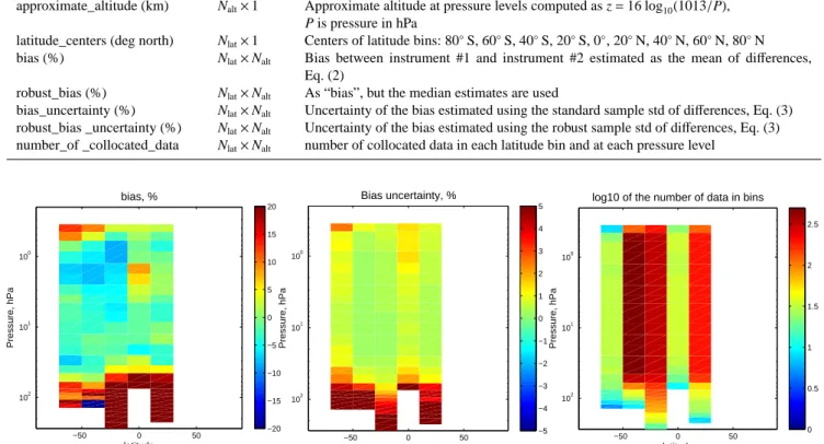
Parameter and unit Dimensions Description/comment Variables air_pressure (hPa) Nalt× 1 The vertical coordinate
approximate_altitude (km) Nalt× 1 Approximate altitude at pressure levels computed as z= 16 log10(1013/P), P is pressure in hPa
latitude_centers (deg north) Nlat× 1 Centers of latitude bins: 80◦S, 60◦S, 40◦S, 20◦S, 0◦, 20◦N, 40◦N, 60◦N, 80◦N bias (%) Nlat× Nalt Bias between instrument #1 and instrument #2 estimated as the mean of differences,
Eq. (2)
robust_bias (%) Nlat× Nalt As “bias”, but the median estimates are used
bias_uncertainty (%) Nlat× Nalt Uncertainty of the bias estimated using the standard sample std of differences, Eq. (3) robust_bias _uncertainty (%) Nlat× Nalt Uncertainty of the bias estimated using the robust sample std of differences, Eq. (3) number_of _collocated_data Nlat× Nalt number of collocated data in each latitude bin and at each pressure level
−50 0 50 100 101 102 latitude Pressure, hPa bias, % −20 −15 −10 −5 0 5 10 15 20 −50 0 50 100 101 102 latitude Pressure, hPa Bias uncertainty, % −5 −4 −3 −2 −1 0 1 2 3 4 5 −50 0 50 100 101 102 latitude Pressure, hPa
log10 of the number of data in bins
0 0.5 1 1.5 2 2.5
Figure 4.A visualization example of bias-related parameters from bias tables, for GOMOS versus OSIRIS in January 2008.
where σ(x1−x2) is the sample standard deviation of the
difference distribution computed in a standard or in a robust way as σ=12(P84− P16), P84 and P16 are 84th and 16th
percentiles, respectively, and N is the number of collocated measurements. In the agreement tables, both parameters b and σb are expressed as percentages. The estimates using the median and percentiles are referred to as “robust” in the created files. Equation (3) represents the standard error of the mean derived assuming uncorrelated randomly sampled measurement pairs. This assumption is appropriate for nearly all HARMOZ pairs due to the properties of data and the method for selecting the collocated measurement. For MIPAS-SCIAMACHY collocations, deviations from assumption are possible; this problem is discussed in Toohey and von Clarmann (2013). The bias is evaluated over the common altitude range of the pair of instruments, using concentration profiles. The bias is evaluated for each month in 20◦ latitude zones from 90◦S to 90◦N. The bias tables
are structured in 15 folders corresponding to the instrument pairs, e.g., “GOMOS_OSIRIS”. They can be found at the same web page http://www.esa-ozone-cci.org/?q=node/161 (or doi:10.5270
/esa-ozone_cci-limb_occultation_profiles-2001_2012-v_1-201308). The folders contain bias ta-bles corresponding to each month in netCDF-4 format. The file names contain information about the year and the month, as well as the instruments and the collo-cation type. For example, the file ESACCI-OZONE-AgreementTable_GOMOS_OSIRIS_200801.nc contains the bias table between GOMOS (x1) and OSIRIS (x2) for
January 2008, for the standard collocation criterion. The files for tight collocation criterion end with “_tight.nc”. The parameters included in the netCDF files are presented in Table 5. A sample visual representation of the main bias parameters is shown in Fig. 4.
The data agreement tables present experimental estimates of biases and their uncertainties. At some locations and sea-sons, the estimated biases can be not statistically significant. Furthermore, discrepancies at upper altitudes are expected (and observed), because of diurnal ozone variations (e.g., Sakazaki et al., 2013, and references therein). The created bias tables are convenient for higher-level analyses, which might aim at detecting statistically significant biases, their latitudinal dependence, and possible drift in time. Examples of such higher-level analyses are presented in Figs. 5 and 6. A
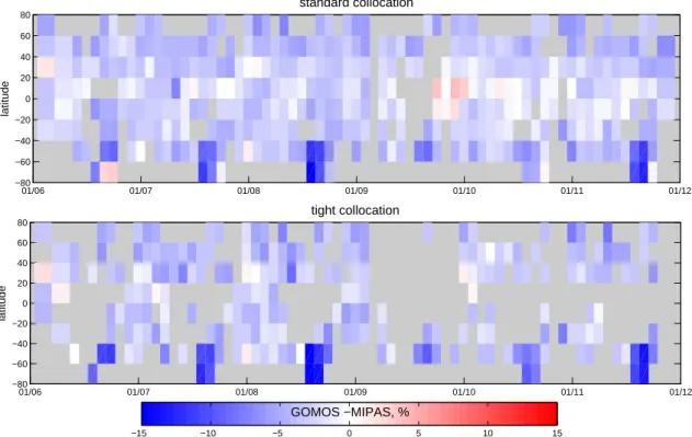
01/06 01/07 01/08 01/09 01/10 01/11 01/12 −80 −60 −40 −20 0 20 40 60 80 latitude standard collocation 01/06 01/07 01/08 01/09 01/10 01/11 01/12 −80 −60 −40 −20 0 20 40 60 80 latitude tight collocation −15 −10 −5 0 5 10 15 GOMOS −MIPAS, %
Figure 5.GOMOS minus MIPAS (in % indicated by color scale) at 30 km, as a function of latitude and time, for standard (top) and tight (bottom) collocation criteria.
detailed analysis of biases and drifts between the instruments will be presented in a separate paper.
Figure 5 shows the time–latitude dependence of biases for “GOMOS minus MIPAS” at 15 hPa (∼ 30 km), for standard and tight collocation criteria. As seen in Fig. 5, the wider collocation criteria do not significantly change the observed biases. At the majority of locations, GOMOS reports slightly smaller ozone values, and this difference is stable in time.
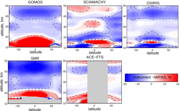
Figure 6 shows mean (over all seasons) biases for 2007– 2008 with respect to MIPAS, as a function of latitude and altitude (subplots show relative differences for “instrument minus MIPAS”). The weighted mean (with uncertainties of individual biases) is used for averaging of monthly bias val-ues. Since the number of collocations with MIPAS over the considered two years is large, the observed differences are statistically significant. Two features can be easily noticed in Fig. 6. First, MIPAS is biased high at altitudes of 40–45 km with respect to all instruments. This feature has also been no-ticed in MIPAS validation studies (Laeng et al., 2012, 2013). Second, a visible enhancement in SCIAMACHY data in the equatorial atmosphere at ∼ 30 km is observed. This feature is unique for SCIAMACHY and also has been observed pre-viously (Mieruch et al., 2012). The presented examples are only simple illustrations of possible analyses using the har-monized dataset and the data agreement tables.
6 Summary
We have described the HARMonized dataset of OZone pro-files (HARMOZ) based on limb and occultation data from six satellite instruments: GOMOS, MIPAS, SCIAMACHY, OSIRIS, SMR and ACE-FTS. The main strength of HAR-MOZ is that it is user-friendly: the independent datasets from individual instruments, which passed thorough quality con-trol, are presented in the same form as far as possible (com-mon vertical grid, com(com-mon parameters, and a com(com-mon data format). Although the datasets are simple and user-friendly, they are also comprehensive: all important parameters at-tributed to individual datasets are presented. Quality of ozone profiles in HARMOZ is characterized by uncertainty esti-mates and the vertical resolution. The created data agree-ment tables provide ready information for various bias and drift analyses. This information is of high importance in joint data analyses and in data merging. A detailed analysis of bi-ases and drifts between the Ozone_cci instruments will be the subject of a future publication.
Between the various datasets, there are ozone measure-ments available for all seasons, various times of day, and good latitudinal coverage. This user-friendly dataset can be very interesting and useful for different analyses and appli-cations, such as data merging, data validation, different inter-comparisons, data assimilation and scientific research. The system has been designed in a flexible and open way in order
latitude altitude, km GOMOS −50 0 50 10 20 30 40 50 latitude SCIAMACHY −50 0 50 10 20 30 40 50 latitude OSIRIS −50 0 50 10 20 30 40 50 latitude altitude, km SMR −50 0 50 10 20 30 40 50 latitude ACE−FTS −50 0 50 10 20 30 40 50 −20 −10 0 10 20 instrument −MIPAS, %
Figure 6.Latitude–altitude dependence of biases with respect to MIPAS (“instrument minus MIPAS” in % is shown in color scale). Dashed black lines indicate ±5 %.
to facilitate the ingestion of additional datasets from other in-struments and/or from other processors, when these become available.
Appendix A
The pressure levels (P, hPa) of the Ozone_cci grid are the following: 450, 400, 350, 300, 250, 200, 170, 150, 130, 115, 100, 90, 80, 70, 50, 40, 30, 20, 15, 10, 7, 5, 4, 3, 2, 1, 1.5, 1, 0.7, 0.5, 0.4, 0.3, 0.2, 0.15, 0.1, 0.07, 0.05, 0.04, 0.03, 0.02, 0.015, 0.01, 0.007, 0.005, 0.004, 0.003, 0.002, 0.0015, 0.001, 0.0007, 0.0005, 0.0004, 0.0003, 0.0002, 0.00015, 0.0001.
The corresponding pressure altitudes z= 16log10(1013/P) in km are the following:
5.64, 6.46, 7.38, 8.46, 9.72, 11.27, 12.4, 13.27, 14.27, 15.12, 16.09, 16.82, 17.64, 18.57, 20.91, 22.46, 24.46, 27.27, 29.27, 32.09, 34.57, 36.91, 38.46, 40.46, 43.27, 48.09, 45.27, 48.09, 50.57, 52.91, 54.46, 56.46, 59.27, 61.27, 64.09, 66.57, 68.91, 70.46, 72.46, 75.27, 77.27, 80.09, 82.57, 84.91, 86.46, 88.46, 91.27, 93.27, 96.09, 98.57, 100.91, 102.46, 104.46, 107.27, 109.27, 112.09.
Acknowledgements. This work has been performed in the framework of the ESA Ozone_cci project.
Edited by: D. Loyola
References
Adams, C., Bourassa, A. E., Bathgate, A. F., McLinden, C. A., Lloyd, N. D., Roth, C. Z., Llewellyn, E. J., Zawodny, J. M., Flit-tner, D. E., Manney, G. L., Daffer, W. H., and Degenstein, D. A.: Characterization of Odin-OSIRIS ozone profiles with the SAGE II dataset, Atmos. Meas. Tech., 6, 1447–1459, doi:10.5194 /amt-6-1447-2013, 2013a.
Adams, C., Bourassa, A. E., Sofieva, V., Froidevaux, L., McLinden, C. A., Hubert, D., Lambert, J. -C., Sioris, C. E., and Degenstein, D. A.: Assessment of Odin-OSIRIS ozone measurements from 2001 to the present using MLS, GOMOS, and ozone sondes, At-mos. Meas. Tech. Discuss., 6, 3819–3857, doi:10.5194 /amtd-6-3819-2013, 2013b.
Bernath, P. F., McElroy, C. T., Abrams, M. C., Boone, C. D., Butler, M., Camy-Peyret, C., Carleer, M., Clerbaux, C., Coheur, P.-F., Colin, R., DeCola, P., DeMazière, M., Drummond, J. R., Dufour, D., Evans, W. F. J., Fast, H., Fussen, D., Gilbert, K., Jennings, D. E., Llewellyn, E. J., Lowe, R. P., Mahieu, E., McConnell, J. C., McHugh, M., McLeod, S. D., Michaud, R., Midwinter, C., Nas-sar, R., Nichitiu, F., Nowlan, C., Rinsland, C. P., Rochon, Y. J., Rowlands, N., Semeniuk, K., Simon, P., Skelton, R., Sloan, J. J., Soucy, M.-A., Strong, K., Tremblay, P., Turnbull, D., Walker, K. A., Walkty, I., Wardle, D. A., Wehrle, V., Zander, R., and Zou, J.: Atmospheric Chemistry Experiment (ACE): Mission overview,
Geophys. Res. Lett., 32, L15S01, doi:10.1029/2005GL022386, 2005.
Bertaux, J. L., Kyrölä, E., Fussen, D., Hauchecorne, A., Dalaudier, F., Sofieva, V., Tamminen, J., Vanhellemont, F., Fanton d’Andon, O., Barrot, G., Mangin, A., Blanot, L., Lebrun, J. C., Pérot, K., Fehr, T., Saavedra, L., Leppelmeier, G. W., and Fraisse, R.: Global ozone monitoring by occultation of stars: an overview of GOMOS measurements on ENVISAT, Atmos. Chem. Phys., 10, 12091–12148, doi:10.5194/acp-10-12091-2010, 2010.
Boone, C. D., Nassar, R., Walker, K. A., Rochon, Y., McLeod, S. D., Rinsland, C. P., and Bernath, P. F.: Retrievals for the at-mospheric chemistry experiment Fourier-transform spectrome-ter, Appl. Optics, 44, 7218–7231, http://ao.osa.org/abstract.cfm?
URI=ao-44-33-7218, 2005.
Bourassa, A. E., Degenstein, D. A., and Llewellyn, E. J.: SASK-TRAN: A spherical geometry radiative transfer code for efficient estimation of limb scattered sunlight, J. Quant. Spectrosc. Ra., 109, 52–73, doi:10.1016/j.jqsrt.2007.07.007, 2008.
Bourassa, A. E., McLinden, C. A., Bathgate, A. F., Elash, B. J., and Degenstein, D. A.: Precision estimate for Odin-OSIRIS limb scatter retrievals, J. Geophys. Res., 117, D04303, doi:10.1029/2011JD016976, 2012.
Bovensmann, H., Burrows, J. P., Buchwitz, M., Frerick, J., Noël, S., Rozanov, V. V., Chance, K. V., and Goede, A. P. H.: SCIAMACHY: Mission Objectives and Measure-ment Modes, J. Atmos. Sci., 56, 127–150, doi:10.1175 /1520-0469(1999)056<0127:SMOAMM>2.0.CO;2, 1999.
Bovensmann, H., Buchwitz, M., Frerick, J., Hoogeveen, R. W. M., Kleipool, Q., Lichtenberg, G., Noel, S., Richter, A., Rozanov, A., Rozanov, V. V., Skupin, J., von Savigny, C., Wuttke, M. W., and Burrows, J. P.: SCIAMACHY on ENVISAT: in-flight opti-cal performance and first results, in: Remote Sensing of Clouds and the Atmosphere VIII, edited by: Schaefer, K., Comeron, A., Carleer, M. R., and Picard, R. H.: Proceedings of the SPIE, 5235, 160–173, 2004.
Bramstedt, K., Noël, S., Bovensmann, H., Gottwald, M., and Bur-rows, J. P.: Precise pointing knowledge for SCIAMACHY solar occultation measurements, Atmos. Meas. Tech., 5, 2867–2880, doi:10.5194/amt-5-2867-2012, 2012.
Degenstein, D. A., Bourassa, A. E., Roth, C. Z., and Llewellyn, E. J.: Limb scatter ozone retrieval from 10 to 60 km using a multiplicative algebraic reconstruction technique, Atmos. Chem. Phys., 9, 6521–6529, doi:10.5194/acp-9-6521-2009, 2009. Doicu, A., Schreier, F., Hilgers, S., von Bargen, A., Slijkhuis,
S., Hess, M., and Aberle, B.: An efficient inversion algo-rithm for atmospheric remote sensing with application to UV limb observations, J. Quant. Spectrosc. Ra., 103, 193–208, doi:10.1016/j.jqsrt.2006.05.007, 2007.
Dupuy, E., Walker, K. A., Kar, J., Boone, C. D., McElroy, C. T., Bernath, P. F., Drummond, J. R., Skelton, R., McLeod, S. D., Hughes, R. C., Nowlan, C. R., Dufour, D. G., Zou, J., Nichitiu, F., Strong, K., Baron, P., Bevilacqua, R. M., Blumenstock, T., Bodeker, G. E., Borsdorff, T., Bourassa, A. E., Bovensmann, H., Boyd, I. S., Bracher, A., Brogniez, C., Burrows, J. P., Catoire, V., Ceccherini, S., Chabrillat, S., Christensen, T., Coffey, M. T., Cortesi, U., Davies, J., De Clercq, C., Degenstein, D. A., De Mazière, M., Demoulin, P., Dodion, J., Firanski, B., Fischer, H., Forbes, G., Froidevaux, L., Fussen, D., Gerard, P., Godin-Beekmann, S., Goutail, F., Granville, J., Griffith, D., Haley, C.
S., Hannigan, J. W., Höpfner, M., Jin, J. J., Jones, A., Jones, N. B., Jucks, K., Kagawa, A., Kasai, Y., Kerzenmacher, T. E., Klein-böhl, A., Klekociuk, A. R., Kramer, I., Küllmann, H., Kuttippu-rath, J., Kyrölä, E., Lambert, J.-C., Livesey, N. J., Llewellyn, E. J., Lloyd, N. D., Mahieu, E., Manney, G. L., Marshall, B. T., Mc-Connell, J. C., McCormick, M. P., McDermid, I. S., McHugh, M., McLinden, C. A., Mellqvist, J., Mizutani, K., Murayama, Y., Murtagh, D. P., Oelhaf, H., Parrish, A., Petelina, S. V., Pic-colo, C., Pommereau, J.-P., Randall, C. E., Robert, C., Roth, C., Schneider, M., Senten, C., Steck, T., Strandberg, A., Strawbridge, K. B., Sussmann, R., Swart, D. P. J., Tarasick, D. W., Taylor, J. R., Tétard, C., Thomason, L. W., Thompson, A. M., Tully, M. B., Urban, J., Vanhellemont, F., Vigouroux, C., von Clarmann, T., von der Gathen, P., von Savigny, C., Waters, J. W., Witte, J. C., Wolff, M., and Zawodny, J. M.: Validation of ozone mea-surements from the Atmospheric Chemistry Experiment (ACE), Atmos. Chem. Phys., 9, 287–343, doi:10.5194/acp-9-287-2009, 2009.
Gurvich, A. S. and Brekhovskikh, V.: A study of turbulence and in-ner waves in the stratosphere based on the observations of stellar scintillations from space: A model of scintillation spectra, Wave. Random Media, 11, 163–181, 2001.
Hegglin, M. I. and Tegtmeier, S.: The SPARC Data Initiative, SPARC Newsl. No. 36, 22, 2010.
Jégou, F., Urban, J., de La Noë, J., Ricaud, P., Le Flochmoën, E., Murtagh, D. P., Eriksson, P., Jones, A., Petelina, S., Llewellyn, E. J., Lloyd, N. D., Haley, C., Lumpe, J., Randall, C., Bevilacqua, R. M., Catoire, V., Huret, N., Berthet, G., Renard, J. B., Strong, K., Davies, J., Mc Elroy, C. T., Goutail, F., and Pommereau, J. P.: Technical Note: Validation of Odin/SMR limb observations of ozone, comparisons with OSIRIS, POAM III, ground-based and balloon-borne instruments, Atmos. Chem. Phys., 8, 3385–3409, doi:10.5194/acp-8-3385-2008, 2008.
Jones, A., Murtagh, D., Urban, J., Eriksson, P., and Rösevall, J.: Intercomparison of Odin/SMR ozone measurements with MI-PAS and balloon sonde data, Can. J. Phys., 85, 1111–1123, doi:10.1139/p07-118, 2007.
Keckhut, P., Hauchecorne, A., Blanot, L., Hocke, K., Godin-Beekmann, S., Bertaux, J.-L., Barrot, G., Kyrölä, E., van Gi-jsel, J. A. E., and Pazmino, A.: Mid-latitude ozone monitoring with the GOMOS-ENVISAT experiment version 5: the noise is-sue, Atmos. Chem. Phys., 10, 11839–11849, doi:10.5194 /acp-10-11839-2010, 2010.
Kyrölä, E., Tamminen, J., Sofieva, V., Bertaux, J. L., Hauchecorne, A., Dalaudier, F., Fussen, D., Vanhellemont, F., Fanton d’Andon, O., Barrot, G., Guirlet, M., Mangin, A., Blanot, L., Fehr, T., Saavedra de Miguel, L., and Fraisse, R.: Retrieval of atmospheric parameters from GOMOS data, Atmos. Chem. Phys., 10, 11881– 11903, doi:10.5194/acp-10-11881-2010, 2010.
Kyrölä, E., Laine, M., Sofieva, V., Tamminen, J., Päivärinta, S.-M., Tukiainen, S., Zawodny, J., and Thomason, L.: Combined SAGE II-GOMOS ozone profile data set for 1984–2011 and trend anal-ysis of the vertical distribution of ozone, Atmos. Chem. Phys., 13, 10645–10658, doi:10.5194/acp-13-10645-2013, 2013. Laeng, A., Grabowski, U., von Clarmann, T., Stiller, G.,
Kell-mann, S., Kiefer, M., Linden, A., Lossow, S. T. B., Bernath, P., Boone, C., Clerbaux, C., Degenstein, D., Fritz, S., Froide-vaux, L., Hervig, M. K., Hoppel, J. L., McHugh, M., Sano, T., Sofieva, V., Suzuki, M., Tamminen, J., Urban, J., Walker, K.,
Weber, M., and Zawodny, J.: Validation of MIPAS IMK/IAA ozone profiles, Quadrenn. Ozone Symp., [online] available at: http://larss.science.yorku.ca/QOS2012pdf/5935.pdf, 2012. Laeng, A., Hubert, D., Verhoelst, T., von Clarmann, T., Dinelli, B.
M., Dudhia, A., Raspollini, P., Stiller, G., Grabowski, U., Kep-pens, A., Kiefer, M., Sofieva, V., Froideveaux, L., Walker, K. A., Lambert, J.-C. and Zehner, C.: The Ozone Climate Change Ini-tiative: Comparison of four Level 2 Processors for the Michelson Interferometer for Passive Atmospheric Sounding (MIPAS), Re-mote Sens. Environ., submitted, 2013.
Lait, L. R.: An alternative form for potential vortic-ity, J. Atmos. Sci., 51, 1754–1759, doi:10.1175 /1520-0469(1994)051<1754:AAFFPV>2.0.CO;2, 1994.
Mieruch, S., Weber, M., von Savigny, C., Rozanov, A., Bovens-mann, H., Burrows, J. P., Bernath, P. F., Boone, C. D., Froide-vaux, L., Gordley, L. L., Mlynczak, M. G., Russell III, J. M., Thomason, L. W., Walker, K. A., and Zawodny, J. M.: Global and long-term comparison of SCIAMACHY limb ozone profiles with correlative satellite data (2002–2008), Atmos. Meas. Tech., 5, 771–788, doi:10.5194/amt-5-771-2012, 2012.
Rahpoe, N., von Savigny, C., Weber, M., Rozanov, A.V., Bovens-mann, H., and Burrows, J. P.: Error budget analysis of SCIAMACHY limb ozone profile retrievals using the SCIA-TRAN model, Atmos. Meas. Tech. Discuss., 6, 4645–4676, doi:10.5194/amtd-6-4645-2013, 2013.
Roth, C. Z., Degenstein, D. A., Bourassa, A. E., and Llewellyn, E. J.: The retrieval of vertical profiles of the ozone number density using Chappuis band absorption information and a multiplica-tive algebraic reconstruction technique, Can. J. Phys., 85, 1225– 1243, doi:10.1139/P07-130, 2007.
Rozanov, A., Rozanov, V., and Burrows, J. P.: A numerical radia-tive transfer model for a spherical planetary atmosphere: com-bined differential–integral approach involving the Picard iter-ative approximation, J. Quant. Spectrosc. Ra., 69, 491–512, doi:10.1016/S0022-4073(00)00100-X, 2001.
Rozanov, V. V., Rozanov, A. V., Kokhanovsky, A. A., and Bur-rows, J. P.: Radiative transfer through terrestrial atmosphere and ocean: Software package SCIATRAN, J. Quant. Spectrosc. Ra., doi:10.1016/j.jqsrt.2013.07.004, in press, 2013.
Sakazaki, T., Fujiwara, M., Mitsuda, C., Imai, K., Manago, N., Naito, Y., Nakamura, T., Akiyoshi, H., Kinnison, D., Sano, T., Suzuki, M., and Shiotani, M.: Diurnal ozone variations in the stratosphere revealed in observations from the Superconduct-ing Submillimeter-Wave Limb-Emission Sounder (SMILES) on board the International Space Station (ISS), J. Geophys. Res.-Atmos., 118, 2991–3006, doi:10.1002/jgrd.50220, 2013. Sofieva, V. F., Tamminen, J., Haario, H., Kyrölä, E., and Lehtinen,
M.: Ozone profile smoothness as a priori information in the in-version of limb measurements, Ann. Geophys., 22, 3411–3420, doi:10.5194/angeo-22-3411-2004, 2004.
Sofieva, V. F., Kan, V., Dalaudier, F., Kyrölä, E., Tamminen, J., Bertaux, J.-L., Hauchecorne, A., Fussen, D., and Vanhellemont, F.: Influence of scintillation on quality of ozone monitoring by GOMOS, Atmos. Chem. Phys., 9, 9197–9207, doi:10.5194 /acp-9-9197-2009, 2009.
Sofieva, V. F., Vira, J., Kyrölä, E., Tamminen, J., Kan, V., Dalaudier, F., Hauchecorne, A., Bertaux, J.-L., Fussen, D., Vanhelle-mont, F., Barrot, G., and Fanton d’Andon, O.: Retrievals from GOMOS stellar occultation measurements using
characteriza-tion of modeling errors, Atmos. Meas. Tech., 3, 1019–1027, doi:10.5194/amt-3-1019-2010, 2010.
Sonkaew, T., Rozanov, V. V., von Savigny, C., Rozanov, A., Bovens-mann, H., and Burrows, J. P.: Cloud sensitivity studies for strato-spheric and lower mesostrato-spheric ozone profile retrievals from mea-surements of limb-scattered solar radiation, Atmos. Meas. Tech., 2, 653–678, doi:10.5194/amt-2-653-2009, 2009.
Tamminen, J., Kyrölä, E., Sofieva, V. F., Laine, M., Bertaux, J.-L., Hauchecorne, A., Dalaudier, F., Fussen, D., Vanhellemont, F., Fanton-d’Andon, O., Barrot, G., Mangin, A., Guirlet, M., Blanot, L., Fehr, T., Saavedra de Miguel, L., and Fraisse, R.: GOMOS data characterisation and error estimation, Atmos. Chem. Phys., 10, 9505–9519, doi:10.5194/acp-10-9505-2010, 2010.
Tegtmeier, S., Hegglin, M. I., Anderson, J., Bourassa, A., Brohede, S., Degenstein, D., Froidevaux, L., Fuller, R., Funke, B., Gille, J., Jones, A., Kasai, Y., Kyrölä, E., Lingenfelser, G., Lumpe, J., Nardi, B., Neu, J., D.Pendlebury, Remsberg, E., Rozanov, A., Smith, L., Toohey, M., Urban, J., Clarmann, T. von, Walker, K. A., and Wang, R.: SPARC Data Initiative: A comparison of ozone climatologies from international satellite limb sounders, J. Geo-phys. Res.-Atmos., 118, doi:10.1002/2013JD019877, 2013. Toohey, M. and von Clarmann, T.: Climatologies from satellite
mea-surements: the impact of orbital sampling on the standard error of the mean, Atmos. Meas. Tech., 6, 937–948, doi:10.5194 /amt-6-937-2013, 2013.
Urban, J., Lautié, N., Le Flochmoën, E., Jiménez, C., Eriksson, P., de La Noë, J., Dupuy, E., Ekström, M., El Amraoui, L., Frisk, U., Murtagh, D., Olberg, M., and Ricaud, P.: Odin/SMR limb obser-vations of stratospheric trace gases: Level 2 processing of ClO, N2O, HNO3, and O3, J. Geophys. Res.-Atmos., 110, D14307, doi:10.1029/2004JD005741, 2005.
Urban, J., Murtagh, D., Lautié, N., Barret, B., Dupuy, E., de La Noë, J., Eriksson, P., Frisk, U., Jones, A., Le Flochmoë, E., Olberg, M., Piccolo, C., Ricaud, P., and Rösevall, J.: Odin/SMR Limb Ob-servations of Trace Gases in the Polar Lower Stratosphere dur-ing 2004–2005, in: ESA Atmospheric Science Conference, 8–12 May 2006, Frascati, Italy, European Space Agency publications ESA-SP-628, ISBN: 92-9092-939-1, ISSN: 1609-042X., 2006. von Clarmann, T., Glatthor, N., Grabowski, U., Höpfner, M.,
Kell-mann, S., Kiefer, M., Linden, A., Mengistu Tsidu, G., Milz, M., Steck, T., Stiller, G. P., Wang, D. Y., Fischer, H., Funke, B., Gil-López, S., and López-Puertas, M.: Retrieval of temper-ature and tangent altitude pointing from limb emission spectra recorded from space by the Michelson Interferometer for Passive Atmospheric Sounding (MIPAS), J. Geophys. Res., 108, 4736, doi:10.1029/2003JD003602, 2003.
von Clarmann, T., Höpfner, M., Kellmann, S., Linden, A., Chauhan, S., Funke, B., Grabowski, U., Glatthor, N., Kiefer, M., Schiefer-decker, T., Stiller, G. P., and Versick, S.: Retrieval of tempera-ture, H2O, O3, HNO3, CH4, N2O, ClONO2and ClO from MIPAS reduced resolution nominal mode limb emission measurements, Atmos. Meas. Tech., 2, 159–175, doi:10.5194/amt-2-159-2009, 2009.
von Savigny, C., Kaiser, J. W., Bovensmann, H., Burrows, J. P., McDermid, I. S., and Leblanc, T.: Spatial and temporal charac-terization of SCIAMACHY limb pointing errors during the first three years of the mission, Atmos. Chem. Phys., 5, 2593–2602, doi:10.5194/acp-5-2593-2005, 2005a.
von Savigny, C., Rozanov, A., Bovensmann, H., Eichmann, K.-U., Noël, S., Rozanov, V., Sinnhuber, B.-M., Weber, M., Burrows, J. P., and Kaiser, J. W.: The Ozone Hole Breakup in September 2002 as Seen by SCIAMACHY on ENVISAT, J. Atmos. Sci., 62, 721–734, doi:10.1175/JAS-3328.1, 2005b.