Air quality impacts and benefits under U.S. policy for air pollution, climate change, and clean energy

(1)

Air Quality Impacts and Benefits under U.S. Policy for Air Pollution, Climate Change, and Clean Energy

by

Rebecca Kaarina Saari

M.A.Sc. Mechanical and Environmental Engineering, University of Toronto, 2007 B.A.Sc. Engineering Science, University of Toronto, 2005

Submitted to the Engineering Systems Division in Partial Fulfillment of the Requirements for the Degree of

DOCTOR OF PHILOSOPHY at the

MASSACHUSETTS INSTITUTE OF TECHNOLOGY June 2015

ARCHNES

MASSACHUSETTS _INSTITUTE OF TECHNOLOLGy

JUL 02 2015

LIB RAR

IES

Signature of Author ...

Signature redacted

C ertified by ...

Engineering Systems Division May 20, 2015

Signature redacted

ffoelle Eckley Selin Esther and Harold E. Edgerton Career Development Assistant Professor of Engineering Systems and Atmospheric Chemistry

A Thesis Committep Chair Certified by ...

Certified by ...

Signature redacted

... .. ..

John)4. Reilly

Senior Lecturer, Sloan School of Management Co-Director of the Joint Program on the Science and P licy of Global Change - ~ Tilysis Committee Member

...

Signature redacted

...

Ronald G. Prinn

TEPCO Professor of Atmospheric Science

Co-Director of the Joint Program on the Science and Policy of Global Change Thesis Committee Member

(2)

(3)

Air Quality Impacts and Benefits under U.S. Policy for Air Pollution,

Climate Change, and Clean Energy

by

Rebecca Kaarina Saari

Submitted to the Engineering Systems Division on May 20, 2015 in Partial Fulfillment of the Requirements for the Degree of

DOCTOR OF PHILOSOPHY

Abstract

Policies that reduce greenhouse gas emissions can also reduce outdoor levels of air pollutants that harm human health by targeting the same emissions sources. However, the design and scale of these policies can affect the distribution and size of air quality impacts, i.e. who gains from pollution reductions and by how much. Traditional air quality impact analysis seeks to address these questions by estimating pollution changes with regional chemical transport models, then applying economic valuations directly to estimates of reduced health risks. In this dissertation, I incorporate and build on this approach by representing the effect of pollution reductions across regions and income groups within a model of the energy system and economy. This new modeling framework represents how climate change and clean energy policy affect pollutant emissions throughout the economy, and how these emissions then affect human health and economic welfare. This methodology allows this thesis to explore the effect of policy design on the distribution of air quality impacts across regions and income groups in three studies. The first study compares air pollutant emissions under state-level carbon emission limits with regional or national implementation, as proposed in the U.S. EPA Clean Power Plan. It finds that the flexible regional and national implementations lower the costs of compliance more than they adversely affect pollutant emissions. The second study compares the costs and air quality co-benefits of two types of national carbon policy: an energy sector policy, and an economy-wide cap-and-trade program. It finds that air quality impacts can completely offset the costs of a cost-effective carbon policy, primarily through gains in the eastern United States. The final study extends the modeling framework to be able to examine the impacts of ozone policy with household income. It finds that inequality in exposure makes ozone reductions relatively more valuable for low income households. As a whole, this work contributes to literature connecting actions to impacts, and identifies an ongoing need to improve our understanding of the connection between

economic activity, policy actions, and pollutant emissions. Noelle E. Selin

Assistant Professor of Engineering Systems and Atmospheric Chemistry

John M. Reilly

Senior Lecturer, Sloan School of Management

(4)

Acknowledgments

It takes a village to prepare a dissertation. I am grateful for the supervision of Noelle Eckley Selin, the insight of my committee members, John Reilly and Ron Prinn, and the support and advice of my Defense Chair, Chris Magee. I was fortunate to participate in several of MIT's vibrant intellectual communities, including Selin Group, the Joint Program on the Science and Policy of Global Change, the Program on Atmosphere, Oceans, and Climate, Atmospheric Chemistry, the Engineering Systems Division, and its student society, ESS, and the BSGE. The three studies that comprise this dissertation were forged through collaboration. I would like to thank North East States for Coordinated Air Use Management (NESCAUM) for their

assistance in selecting the policy scenarios for Essay 2. I thank Tammy Thompson, Sebastian Rausch, Justin Caron, and Kyung-Min Nam for their previous work in developing economic, health, and air quality modeling methodologies and analyses that I adapted or incorporated into this work.

Various aspects of this work were funded in part by the US EPA under the Science to Achieve Results (STAR) program (#R834279); MIT's Leading Technology and Policy Initiative; MIT's Joint Program on the Science and Policy of Global Change and its consortium of industrial and foundation sponsors (see: http://globalchange.mit.edu/sponsors/all); US Department of Energy Office of Science grant DE-FG02-94ER61937; the MIT Energy Initiative Total Energy

Fellowship; the MIT Martin Family Society Fellowship; the MIT Energy Initiative Seed Fund program. Although the research described has been funded in part by the US EPA, it has not been subjected to any EPA review and therefore does not necessarily reflect the views of the Agency, and no official endorsement should be inferred.

All of this work was supported by my family, with love to Brian, Jonathan, Matti, Cathy, Maija,

(5)

List of Figures

Figure 1-1: USREP Regions used in Regional Implementation... 23

Figure 1-2: Change in Fossil Input to Electricity by Scenario Compared to Business-as-Usual in 2 0 2 0 ... 2 4 Figure 1-3: Change in Fossil Input to Other Sectors by Scenario Compared to Business-as-Usual in 2 0 2 0 . ... 2 4 Figure 1-4: Change in Pollutant Emissions by Scenario Compared to Business-as-Usual in 2020.

... 2 8

Figure 1-5: Change in Total Primary PM2.5 Emissions Compared to State in 2020. (a) National

vs. State (b) R egional vs. State. ... 29

Figure 2-1: Integrated assessment framework for estimating air quality co-benefits of US climate p o licy ... 3 8

Figure 2-2: R egions of U SRE P... 41 Figure 2-3: Ratio of median co-benefits to the magnitude of policy costs for the CES (%).

Median CES co-benefits range from 1% (in California) to 10% (in New York) of the magnitude

o f p o licy co sts. ... 5 5

Figure 2-4: Ratio of median co-benefits to the magnitude of policy costs for the CAT (%). ... 56 Figure 2-5: CES median difference in the share of co-benefits from the share of mortalities (%).

... 5 8

Figure 2-6: CAT median difference in the share of co-benefits from the share of mortalities (%).

... 5 9

Figure 3-1: Decreasing pattern with household income of U.S. national incidence rate of ozone-related mortalities in the base year (2005) and Policy Scenario (2014). ... 77

Figure 3-2: Percent welfare gain by household income group. Solid blue line uses VSL valuation for reduced m ortality risk ... 78

Figure 3-3: Effect of accounting for differential ozone reductions across household income groups on relative w elfare gain... 79

Figure 3-4: Normalized percent per capita welfare gain of the Policy Scenario by household income group. Blue solid line employs the VSL-based valuation; red dashed line employs the

(9)

(10)

List of Tables

Table 1-1: USREP Model Details: Household, and Sectoral Breakdown and Primary Input Factors; Regional Breakdown for the Regional-Level Implementation... 21 Table 1-2: Change in Pollutant Emissions from Electricity by Scenario in 2020 vs. BAU

(thousand tons/year)... 26

Table 1-3: Change in Total Pollutant Emissions by Scenario in 2020 vs. BAU (thousand

to n s/y ear)... 2 7

Table 1-4: Percent Change in Emissions Reductions Compared to State in 2020 ... 27 Table 2-1: USREP Model Details. Regional, Household, and Sectoral Breakdown and Primary In p u t F acto rs ... 4 0 Table 2-2. Endpoints, epidemiologic studies, and valuations used for fine particulate matter health impacts, following US EPA (2012) ... 43 Table 2-3: Median co-benefits of each policy (total, per capita, and per ton of mitigated CO2

em issions) [range in square brackets]... 50

Table 2-4: Co-benefits, costs, and net co-benefits in billions 2005$... 51

Table 3-1: Health impact functions and valuations ... 71

Table 3-2: USREP Model Details: Regional, Household, and Sectoral Breakdown and Primary In p u t F acto rs ... 7 3

(11)

Introduction

This dissertation comprises three studies on the topic of air quality impacts and co-benefits under policy for clean air, clean energy, and climate change. Its aim is to develop a methodological framework that can explore how the design of policy affects the distribution of air quality impacts and benefits. Its contributions are thus methodological and policy-relevant.

This dissertation makes a methodological contribution to the strand of the broader sustainability science literature that studies the links between the grand sustainability challenges of air

pollution, clean energy, and climate change. The sustainability science literature listed its core questions in Kates et al. (2001), including the need to illuminate the dynamics and incentives of sustainable systems. Scholars of air quality impacts have pointed to interactions with climate change and climate policy as a significant link in assessing sustainable solutions, while citing epistemic divides as a reason that air quality co-benefits have lacked policy traction. Nemet et al. (2010) and Thompson et al. (2014) describe the need to link methods from climate policy

analysis to air quality impacts in order to capture the full policy-to-impacts pathway and illuminate the dynamics and incentives that influence the air quality co-benefits of climate policy.

(12)

produce hourly, gridded emissions, the Sparse Matrix Operating Kernel Emissions model, or SMOKE (CMAS 2010). It converts emissions into ambient pollutant concentrations with a regional chemical transport model, the Comprehensive Air Quality Model with extensions, CAMx (Environ International Corporation 2013). It estimates human health impacts related to two criteria air contaminants, ozone and fine particulate matter, using the Benefits Mapping and Analysis Program, BenMAP (Abt Associates, Inc. 2012). This dissertation's innovation is to add an energy and climate policy analysis model, the U.S. Regional Energy Policy Model (Rausch et al. 2010), to the start and end of this process. Completing this loop allows us to capture

feedbacks in the economy that affect economy-wide pollutant emissions under policy, and to capture the nonlinear chemistry and concentration-response functions that transform emissions into human impacts.

Representing these linkages and feedbacks within a common framework allows us to complement existing studies of the air quality impacts of policy, while also answering new questions about how policy design affects the distribution of these impacts. This dissertation comprises three studies that each develops a new aspect of this modeling framework in order to answer a different policy-relevant question.

First Essay

Air Quality under State-Level Limits or Regional Trading to Regulate CO2from Existing Power

Plants

The methodological development of the first essay is to link the economic output of a

Computable General Equilibrium (CGE) economic model, USREP, with state-level detail, to a regulatory emissions modeling system, SMOKE. Typically, in air quality co-benefits analysis, a model like SMOKE would be driven by emissions changes from engineering estimates or electricity modeling results that are limited to the electricity sector. Our approach complements this technique by using an economy-wide model to capture emissions changes outside of the electricity sector, e.g., from emissions due to extracting, processing, and transporting fossil fuels. The technique follows Thompson et al. (2014), matching sectoral input and output in USREP to detailed source classification codes in SMOKE to develop a future emissions inventory under

(13)

Developing this approach allows us to compare economy-wide policy costs and emissions changes under U.S. energy policy. Specifically, we study the type of state-level carbon intensity limits proposed in the EPA Clean Power Plan (CPP), and compare the effect of state, regional, and national compliance. This question is motivated by the fact that the CPP allows this flexibility in achieving compliance, and that this will likely reduce costs but can increase

pollutant emissions, potentially shifting emissions to regions with elevated pollutant damages. In other words, the net effect on co-benefits and costs is unclear.

This study suggests that there are important emissions reductions from non-electricity sector sources, accounting for up to 15% of fine particulate matter reductions and up to one third to two thirds of reductions in carbon monoxide, volatile organic compounds, and ammonia. It also suggests that the more flexible implementations of the CPP, including national and regional compliance, might increase net co-benefits. However, to make a commensurate comparison, one would have to convert emissions changes into co-benefits. Complex nonlinear relationships link pollutant emissions to their resulting health and economic impacts. The Second Essay completes this next link in order to compare costs and air quality co-benefits for two types of carbon policy.

Second Essay

A Self-Consistent Method to Assess Air Quality Co-Benefits

from

U.S. Climate Policies

The methodological development of the second essay is the mirror of the first: it links the output of an air quality impact modeling system to a Computable General Equilibrium (CGE) economic model, USREP. Using the air quality modeling system captures nonlinear chemical

transformation and concentration-response relationships, as is done in regulatory air quality impact analysis. Representing these impacts within a CGE framework complements this approach by estimating the economic welfare impacts of pollution-related health effects under the constraints of multiple interacting policies, limited resources, and price responses. This approach also addresses a gap, identified by Nemet et al. (2010), that models commonly used to assess climate policies, like CGE models (Paltsev and Capros 2013), do not include air quality

(14)

Currently, the co-benefits literature spans many methods and many carbon policy types, making it difficult to draw comparisons (Nemet et al. 2010). The self-consistency offered by this new modeling framework allows us to directly compare costs and co-benefits for multiple policy types. The second essay employs this framework to ask whether co-benefits can exceed the costs of an energy sector or economy-wide carbon policy. The energy sector policy limits CO2

emissions by specifying a percentage of electricity sales from low-carbon sources. The economy-wide policy limits the same amount of CO2 emissions but allows reductions from anywhere in the economy via a cap-and-trade program. We find that the more cost-effective cap-and-trade instrument has median air quality co-benefits that exceed its policy costs. We find that including air quality co-benefits shifts the distributional effects of the policy to favor eastern states. Finally, we find that general equilibrium effects have a relatively minor effect on the distribution of air quality co-benefits, but can shift them slightly toward high productivity regions.

This study explores the distribution of air quality impacts by location. Another key dimension of a policy's distributional implications is how its effects vary with income. The third essay

introduces the ability to distinguish air quality impacts not only by location but also by income group.

Third Essay

Human Health and Economic Impacts of Ozone Reductions by Income Group

The methodological development of the third essay is to represent the health-related economic impacts of ozone pollution with household income. It builds on USREP's ability to track economic welfare among representative households in nine income categories. Along with economy and environment, social equity is a key pillar of sustainability, meaning that representing economy-wide effects of environmental policy with income is needed, though

empirical and theoretical challenges remain. This method allows us to explore the consequences of current approaches common in CGE modeling and regulatory analysis for the assessment of ozone policy with income.

(15)

2014). We use this approach to estimate the relative economic value of ozone reductions by household income category. We use a modeling scenario that compares 2005 ozone levels to a suite of reductions that were planned for 2014. We compare the effect of potential outcomes of policy - like unequal reductions with income, and delay - with different valuation techniques. We find that ozone reductions appear relatively more valuable to low income households, who are also relatively more affected by delay. The factor having the greatest effect on the relative value of reductions was the valuation technique, followed by delay and the effect of accounting for disproportionate ozone reductions among low-income households.

Conclusion

This dissertation develops a modeling framework that can be used to aid the analysis of climate, energy, and air quality policy in terms of the three pillars of sustainability: economy,

environment, and equity. It illuminates the dynamics between climate policy and air quality impacts and their distributions under different types of economic incentives. Using this new technique serves to bolster some findings while highlighting remaining gaps. For example, the second essay reaffirms the prevalent claim that air quality co-benefits can exceed policy costs for a cost-effective instrument, this time with a more self-consistent comparison. Conversely, the first essay finds that energy-sector models may miss up to 15% of PM2.5 reductions, and even

more reductions of precursor contaminants. The third finds that, while ozone-related health risk inequality persists, there are perhaps greater opportunities to understand and address economic inequality.

Some of the co-benefits literature motivates its work as a means to reduce the apparent costs of climate mitigation, to inform multi-pollutant management, or to produce assessments of

sustainable development and risk inequality (Ravishankara, Dawson, and Winner 2012; Nemet, Holloway, and Meier 2010; Fann et al. 2011). This dissertation provides insights that bear on the relative significance of air quality co-benefits to climate mitigation costs, the interplay of CO2

reductions and pollutant emissions, and the intersection of environmental policy and income inequality. In so doing, it serves to quantify and compare the relative importance of several ways

(16)

(17)

First Essay

1. Air Quality under State-Level Limits or Regional Trading to Regulate C02

from Existing Power Plants

(18)

INTRODUCTION

The energy sector is a significant source of greenhouse gas emissions that cause climate change as well as air pollutants that harm human health (Burtraw et al. 2003). The EPA recently proposed the Clean Power Plan (CPP) to limit emissions of CO2 from existing power plants

(U.S. Environmental Protection Agency 2014a). The CPP proposes state-specific carbon

intensity limits, but allows regional compliance. For example, several states could work together to meet a combined limit. The CPP is also expected to yield significant benefits for ozone and

fine particulate matter, in excess of policy costs and direct domestic benefits from reducing CO₂

(U.S. Environmental Protection Agency 2014a). If regional or national compliance results from

the CPP, it has the potential to reduce both costs and air quality impacts, likely at different rates. Previous analyses of the CPP have focused on energy-sector emissions (U.S. Environmental Protection Agency 2014a; Driscoll et al. 2014), but changes to emissions in non-energy sectors can also be significant (Rausch, Metcalf, and Reilly 2011; Thompson et al. 2014), including upstream effects in coal producing states (Larsen 2014). Here, we build on previous analyses by

capturing economy-wide emissions changes and directly exploring the effect of state-level, regional, or national implementation on air pollutants. We use this analysis to examine the effect

of the geographic scale of trading to meet state-level CO2 limits on the size and distribution of air

pollutant emissions.

The proposed EPA CPP designates state-level CO2 intensity limits, but permits states to achieve

"regional compliance" through emissions trading. The ability to trade will likely have different effects on the costs and air quality co-benefits of the rule. Trading will likely lower the policy costs by increasing access to low-cost abatement opportunities. Trading is also likely to affect air quality co-benefits. The response of air quality impacts is complicated by that fact that the

marginal damages of pollution vary by source, time, and location (Tietenberg 1995). Some studies suggest accounting for this can increase the benefits and economic efficiency of markets for clean air such as the NOx Budget Program or Acid Rain Trading program (Mesbah, Hakami, and Schott 2014; Spencer Banzhaf, Burtraw, and Palmer 2004; Mauzerall et al. 2005; Tong et al.

2006; Graff Zivin, Kotchen, and Mansur 2014; Muller and Mendelsohn 2009). Conversely,

(19)

complicated effect, and may not be socially beneficial (Muller 2012). Allowing trading is likely to affect costs more than co-benefits, based on previous studies comparing energy sector and economy-wide policies (Thompson et al. 2014; Saari et al. 2015). Thus, the spatial extent of trading for a carbon policy will likely yield cost savings and may reduce air quality co-benefits. Therefore we hypothesize that allowing trading will decrease costs but may increase pollutant emissions.

In particular, trading may reduce air quality co-benefits in already polluted or populated areas where the damages from pollution are high. Trading will tend to shift emissions to areas with low marginal abatement costs for C02, but some of these areas might also have high marginal damages from pollution. The potential for emissions trading to lead to pollution "hotspots", or areas of high concentrations, has been studied for toxic pollutants (Adelman 2013) and criteria pollutants emitted from the energy sector as in the acid rain trading program (Burtraw and Mansur 1999; Shadbegian, Gray, and Morgan 2007). A recent study showed that SO2 trading

shifted emissions from low to high damage areas (Henry, Muller, and Mendelsohn 2011). Others have explored whether the differing incentives of state-level or regional-level compliance might lead to 'environmental browning' (Bellas and Lange 2008). The air quality co-benefits of the CPP provide a complex case for several reasons. First, the trading will focus on CO2 while the air

quality impacts will result from multiple co-emitted pollutants. Second, states are subject to non-uniform targets that depend on existing conditions, opportunities, and commitments. The

interaction of the differing limits, costs, and damages will determine how the extent of trading affects high-damage areas. Since air quality impacts comprise a large share of the benefits, the potential outcome of trading is important to explore because it affects the distributional

implications of this policy.

Here, we explore how potential trading to meet state-level CO2 limits will affect the size and distribution of air pollutant emissions. We implement these policies using a recently developed

(20)

examine trade-offs in policy cost and air quality improvement at various scales. We draw conclusions from this work to inform strategies for policy implementation.

INTEGRATED ASSESSMENT METHODS Integrated Modeling Framework

We model policies and resulting emissions using an integrated assessment framework similar to Thompson et al. (2014). This framework links the economic model USREP, used to estimate policy costs and economy-wide CO2 emissions changes, to an advanced system for modeling air

quality impacts.

The U.S. Regional Energy Policy Model

USREP is a computable general equilibrium (CGE) economic model designed to study the

long-run dynamics of resource allocation and income distribution under energy and environmental policy. It is a recursive dynamic model that calculates the commodity prices that support equilibrium between supply and demand in all markets. USREP is suited to exploring the environmental impacts and distributional implications of U.S. national and sub-national energy policy because it includes rich detail in its energy sector, relates production to emissions of greenhouse gases, and represents multiple sectors, regions, and income groups. The version of

USREP used in this study features the ability to simulate state-specific targets, updated 2012

energy and economic data, and international trade; it also solves in two-year periods (Caron, Rausch, and Winchester 2015; Caron, Metcalf, and Reilly 2015). This state-level version was developed recently and its results are considered to be preliminary. This means that we use it here to demonstrate the methodology, and to examine the general effects of the policy

implementation scale, but not to predict specific state-level outcomes. Previous studies using

USREP: describe its structure and inputs; present climate change and energy policy applications;

test sensitivity to inputs, structure and assumptions; and compare its performance to other energy and economic models (Rausch, Metcalf, and Reilly 2011; Thompson et al. 2014; Saari et al.

2015; Caron, Rausch, and Winchester 2015; Rausch and Mowers 2014; Rausch et al. 2010;

(21)

Table 1-1: USREP Model Details: Household, and Sectoral Breakdown and Primary Input

Factors; Regional Breakdown for the Regional-Level Implementation

Regions

Pacific (PACIF) California (CA) Alaska (AK)

Mountain (MOUNT) North Central (NCENT) Texas (TX)

South Central (SCENT) North East (NEAS)

South East (SEAST)

Florida (FL) New York (NY) New England (NENGL)

Primary production factors Capital

Labor

Coal resources Natural gas resources Crude oil resources Hydro resources Nuclear resources Land Wind Sectors Non-Energy Agriculture (AGR) Services (SRV)

Energy-intensive products (EIS) Other industries products (OTH) Commercial transportation (TRN) Passenger vehicle transportation (TRN) Final demand sectors

Household demand Government demand Investment demand Energy

Coal (COL)

Natural gas (GAS) Crude oil (CRU) Refined oil (OIL) Electric: Fossil (ELE) Electric: Nuclear (NUC) Electric: Hydro (HYD) Advanced Technologies

Linking USREP to Pollutant Emissions

Following Thompson et al. (2014), we link production in USREP to the relevant emissions sources in a national emissions inventory for 2005. This emissions inventory is temporally processed and speciated on a 36-km grid of the continental U.S. using the same year-long 2005 modeling episode described in Thompson et al. (2014), and documented and evaluated against ambient monitors in U.S. EPA (2011 b). Here, we use the state-level output from USREP in 2020 to scale the corresponding detailed anthropogenic point and area sources in each state. We compare the changes in fuels used in the electricity sector, energy intensive industries, and other industry, as well as the outputs of the sectors of agriculture, electricity, fossil fuel production, service, transportation, and other manufacturing. These variables are mapped to hundreds of

Household income classes

($1,000 of annual income) <10 10-15 15-25 25-30 30-50 50-75 75-100 100-150 >150

(22)

emissions across the economy. For example, reducing demand for coal in power generation affects the pollutant emissions associated with mining, processing, and transporting coal. A disadvantage is that this framework does not endogenously include pollution-specific post-process abatement options to reduce pollution under future air quality policies. Thus, our scenarios are scaled from emissions factors based on current pollution abatement levels and regulations. They should thus be interpreted as the effect of the carbon policies apart from any decisions regarding air pollution, though there may be important interactions.

We use these scaling factors in the SMOKE model to produce gridded, hourly emissions for each scenario in the year 2020. We estimate changes to criteria air contaminants and important

precursors for the formation of fine particulate matter and ozone, including sulfur dioxide (SO2), nitrogen oxides (NOx), fine particulate matter (PM2.5), carbon monoxide (CO), volatile organic

compounds (VOC), and ammonia (NH3).

Analyzing State-Level, Regional, and National Policy Compliance

In this analysis, we represent the state-level limits for the electricity sector defined in the CPP. These are rate-based intensity limits which we convert to equivalent mass-based limits, as permitted by the rule. The EPA had computed targets based on four building blocks for

reductions, including: 1. heat rate improvements; 2. re-dispatch to lower emission sources (e.g., switch from coal to natural gas); 3. expanded low-carbon generation (e.g., increase renewables penetration); and 4. demand-side measures. States are free to choose their means of compliance.

By imposing state-level caps for CO2 from electricity, our model allows states to endogenously

choose between building blocks two through four to meet their targets.

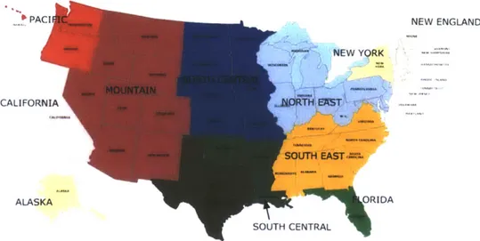
We compare three policy scenarios: state-level compliance (State), regional trading (Regional), and national trading (National). In the Regional scenario, states can meet their combined limits within 12 regions which were determined to capture differences in electricity costs and are depicted in Figure 1-1 (Rausch et al. 2010). These regions comprise the states of California, Florida, New York, and Texas, as well as several multistate aggregations. In the National

scenario, states can trade with any other state. We compare each policy scenario to the Business-as-Usual (BAU). The resulting changes in production are used to estimate future emissions for

(23)

each policy. We model emissions in the continental U.S. only, which excludes Alaska and Hawaii.

NEW ENGLAND

CALIFORNIA '4

ALASKA

Figure 1-1: USREP Regions used in Regional Implementation.

They are the aggregation of the following states: NEW ENGLAND = Maine, New Hampshire, Vermont,

Massachusetts, Connecticut, Rhode Island; SOUTH EAST = Virginia, Kentucky, North Carolina, Tennessee, South Carolina, Georgia, Alabama, Mississippi; NORTH EAST = West Virginia, Delaware, Maryland, Wisconsin, Illinois, Michigan, Indiana, Ohio, Pennsylvania, New Jersey, District of Columbia; SOUTH CENTRAL = Oklahoma, Arkansas, Louisiana; NORTH CENTRAL = Missouri, North Dakota, South Dakota, Nebraska, Kansas, Minnesota, Iowa; MOUNTAIN = Montana, Idaho, Wyoming, Nevada, Utah, Colorado, Arizona, New Mexico; PACIFIC =

Oregon, Washington, Hawaii.

RESULTS OF COMPLIANCE SCALE ON PRODUCTION Effects on Fossil Fuel Input to Electricity and Other Sectors

The scale of compliance, be it national, regional, or state, has different effects on fossil fuels used in electricity production, as shown in Figure 1-2. The largest effects are to coal, which decreases by about 13% in 2020 compared to Business-as-Usual. National and regional compliance both reduce about 1 percentage point more coal use in electricity production than

state-level compliance. For both natural gas and oil, the regional and state level implementations have similar, larger decreases in fossil fuel use than the national implementation.

(24)

Fossil Input to Electricity vs. BAU in 2020 (%)

National Regional State

0% -2% -4% -6% -8% -10% -12% -14% -16%

U Coal N Natural Gas U Oil

Figure 1-2: Change in Fossil Input to Electricity by Scenario Compared to Business-as-Usual in

2020.

As the use of fossil fuels decreases in electricity generation, it increases slightly in other sectors. Fossil fuel use increases in energy intensive industries and other activities between 0% and 1%. These increases do not compensate for the reduced fossil fuel use in electricity, as the majority of fossil fuels are used in the electricity sector, meaning that overall fossil fuel use in the economy decreases. For example, the decrease in coal use in electricity is over 100 times greater than the increase in coal used in electricity intensive industries.

Fossil Input to Other Sectors vs. BAU in 2020

(%)

1.0%

0.5%L

L

t. _h

0.0%

National Regional State National Regional State

Energy Intensive Other

M Coal 0 Natural Gas M Oil

Figure 1-3: Change in Fossil Input to Other Sectors by Scenario Compared to Business-as-Usual

(25)

Effects on Economic Output

For most sectors, the policy scenarios reduce economic output compared to Business-as-Usual. Output is changed by less than 0.2%, with the exception of fossil-powered electricity generation and fossil production, particularly coal and natural gas production. The majority of sectors have their output reduced by an amount that increases inversely with the extent of trading, from national, to regional, to state. In other words, the more flexible implementations have a smaller effect on economic output from fossil-based power generation. This relationship is not linear. In these initial findings, Regional and State are more similar to each other in their main effect on

economic output, i.e., to fossil-fueled power generation, than they are to National. This trend also holds for most other sectors as well, with the national-level implementation having the smallest

effect on all sectors, except that the regional implementation has slightly smaller effects on agriculture, refined oil, and service. Similarly, the regional-level implememtation has smaller effects on all sectors than the state-level, with the exception of agriculture and energy-intensive industries.

Effects on Economic Welfare Per Capita

The more flexible the implementation, the lower is the estimated consumption loss from the policy. Initial estimates of the consumption loss per capita in 2020 are inversely proportional to the extent of trading. Moving from state-level compliance to regional compliance reduces costs

by about 20%, and allowing national compliance reduces costs by about 50%. Reduction in Energy Sector Emissions by Pollutant

Emissions from the electricity sector are reduced for all pollutants in all implementation scenarios, as shown in Table 1-2. Compared to Business-as-Usual, by pollutant, reductions are highest for SO2, followed by NOx, CO, primary PM2.5, VOC, and ammonia (NH3). For most pollutants, reductions are similar across scenarios, except for SO2 and CO; for both of these, National has a smaller effect than State or Regional, which echoes their effects on output from electricity production.

(26)

Table 1-2: Change in Pollutant Emissions from Electricity by Scenario in 2020 vs. BAU

(thousand tons/year)

Scenario SO2 NOx PM2.5 Co VOC NH3

National -932 -370 -47 -53 -3 -2

Regional -998 -378 -49 -85 -4 -2

State -993 -331 -48 -80 -3 -2

Percent Reductions from Fossil Fuel Based Electricity (%)

National -11% -12% -12% -10% -10% -8%

Regional -12% -12% -12% -16% -11% -10%

State -12% -11% -12% -15% -10% -9%

The total emissions reductions in Table 1-2 correspond to a percentage reduction between 8% and 16% across these pollutants. For every pollutant, the Regional scenario reduces the most emissions. The more flexible National scenario always has higher emissions than the Regional scenario, but the results of the State scenario are more mixed. Overall, there is a relatively small percentage change between scenarios. The reductions are within 1 or 2 percentage points for all pollutants but CO. This result is consistent with the EPA's assessment of the Clean Power Plan, and Driscoll's assessment of three related policy scenarios (U.S. Environmental Protection Agency 2014a; Driscoll et al. 2014).

Total Emissions Reductions by Scenario and Pollutant

Considering emissions from all sources, total emissions of all pollutants are reduced under all scenarios compared to BAU, as shown in Table 1-3 and Figure 1-4. This means that the net effect of the policy is to reduce pollutant emissions overall, though emissions from some sources may increase; for example, emissions of SO2 from area sources increases under the policy, which

may be due to the increase in coal use outside the electricity sector. While the majority of emissions reductions come from the electricity sector, the policy scenarios indirectly affect emissions in energy intensive industries, transportation, and other sectors. Overall, the electricity sector accounts for nearly 100% of reductions in SO2 and NOx, 85%-92% in primary PM2.5, and

(27)

Table 1-3: Change in Total Pollutant Emissions by Scenario in 2020 vs. BAU (thousand

tons/year)

SO2 NOx PM2.5 CO VOC NH3

Total Emissions Reductions

National -932 -375 -52 -81 -8 -2

Regional -1,000 -387 -56 -125 -10 -3

State -999 -341 -56 -123 -12 -3

Percent of Total Emissions Reductions from Electricity

National 100% 99% 92% 65% 45% 66%

Regional 100% 98% 88% 68% 36% 59%

State 99% 97% 85% 65% 27% 48%

Overall, the percent of total reductions are small except for SO2, followed by NOx and primary

PM2.5, as shown in Figure 1-4. For all pollutants except NOx, Regional and State have similar,

lower emissions than National. Moving from State level compliance to Regional or National will typically increase emissions, i.e., lower the percent reductions. Just as costs drop with a more flexible policy, so does the size of emissions reductions. Table 1-4 compares the size of total emissions reductions under National, Regional, and State. For example, a National

implementation will decrease SO2 reductions from 999 to 932, or by 7%. National gains 10%

more NOx reductions, but erodes 8% of primary PM2.5 reductions and about 30% of reductions

in CO, VOC, and ammonia.

Table 1-4: Percent Change in Emissions Reductions Compared to State in 2020

SO2 NOx PM2.5 CO VOC NH3

National vs. State 7% -10% 8% 34% 40% 31%

(28)

Total Emissions in 2020 vs. BAU (%) S02 NOX PM2.5 CO VOC NH3 0% --2% --4% --6%

n National U Regional U State

-8%

Figure 1-4: Change in Pollutant Emissions by Scenario Compared to Business-as-Usual in 2020. Emissions Reductions by Location

Figure 1-5 shows the effect of National vs. State or Regional vs. State implementations on the change in total primary PM2.5 emissions in 2020. Primary PM2.5 emissions will not represent

total ambient PM2.5, much of which will be formed from precursor emissions, and these

preliminary results are not meant to predict outcomes in a given state. Nonetheless, they can be used to hypothesize whether the air quality co-benefits may shift to high damage areas. The majority of benefits will be due to fine particulate matter. Fann et al. (2011) mapped the public health burden from PM2.5 and ozone, showing the highest damages in the Eastern U.S. and

California. Comparing National vs. State, the more flexible policy does qualitatively appear to increase emissions more in high-damage than low-damage areas. Regional vs. State

implementation has a similar but less pronounced pattern.

DISCUSSION

Regardless of their implementation, the state-level carbon intensity limits explored here are estimated to decrease fossil fuel use in electricity production, decrease economic output from fossil-powered electricity, impose a policy cost, and decrease pollutant emissions compared to Business-as-Usual. We compare three different implementation scenarios, State, Regional, and National, representing three different scales of compliance. National, the most flexible approach, has the lowest policy cost, and the least effect on fossil fuel use, economic output, and total

(29)

emissions for each pollutant. The effect of a more flexible policy implementation is generally to lower costs, increase economic output, and increase pollutant emissions.

Annual Emissions of PM

2

.

5

National vs. State

a "

30

24 18 12

6

0

-6

-12

-18

-24

-30

0 4j C 0

E

W (a)

Annual Emissions of

PM

2

.

5

Regional vs. State

li//

30

24 18 12 6

0

-6 -12

-18

-24

-30

0

E

W .1-(b)

(30)

All implementation scenarios reduce emissions of all pollutants compared to BAU. The largest

reductions are to SO2, NOx, CO, and primary PM2.5. The largest impact of each policy scenario

is to electricity generated from fossil fuels. Coal use in this sector drops by 13%, its output drops, and its emissions drop between 8% and 16%.

Unlike previous analyses (Driscoll et al. 2014; U.S. Environmental Protection Agency 2014a), we capture non-electricity sector emissions changes. Reductions in fossil-based electricity account for 85%-100% of the total emissions reductions in S02, NOx, and primary PM2.5. Thus,

previous analyses that only focus on this sector will capture most of the air quality benefits. Nonetheless, non-electricity sector effects add an additional 15% reduction in primary PM2.5, and

one third to two thirds additional reductions of CO, VOC and ammonia, which are important precursors of ozone and secondary fine particulate matter. Thus, capturing these economy-wide emissions can increase air quality co-benefits estimates compared to previous analyses.

Economy-wide, the largest percent emissions reductions compared to BAU are from SO2 (7%), NOx (1%), and primary PM2.5 (1%). Emissions are fairly similar under all three implementation

scenarios. National reduces fewer emissions than State or Regional for nearly all pollutants, which follows from its relative effects on economic activity. The exception is NOx, which is slightly higher under State than National or Regional. This small increase in NOx from

electricity generation and industrial sectors under a carbon policy was also found by Rudokas et al. (2015). In industry, they attribute this to a switch to combined heat and power. In the

electricity sector, they cite delayed investments, reduced efficiency due to carbon capture, and leakage outside the Clean Air Interstate Rule area. In our case, State has higher NOx emissions perhaps due to its higher switching from coal to natural gas fired electricity that can have higher NOx emission factors even though natural gas combustion typically emits less SO2 and primary

PM₂.5.

The effect of the implementation scenario on costs is much higher than the effect on emissions, on a percentage basis. National costs about 50% less than State, while it loses around 10% of SO2 and PM2.5 reductions, but gains about 10% in NOx reductions. This suggests that allowing a

(31)

distribution of emissions by location, it is also possible that National could tend to shift

emissions to high-damage areas where mortality risks from fine particulate are already relatively elevated. In order to examine these competing effects, a commensurate comparison of costs and co-benefits would be needed to compute the economic benefits from these foregone emissions reductions.

Our estimated emissions reductions are comparable with EPA's analysis of the Clean Power Plan, which quotes results for NOx, SO2, and PM2.5. For the regional compliance case, our

reductions are 8% higher for NOx and 13% lower for PM2.5. For state-level compliance, our

reductions are 11% and 22% lower for NOx and PM2.5, respectively. Conversely, our estimates of SO2 are higher by 71% and 66% for Regional and State, respectively. Our higher estimates of SO2 reductions are mainly attributed to our use of 2005-level pollution control and policy, which

does not include regulations like the Mercury and Air Toxics Standard (MATS) that is expected to reduce power-sector SO2 emissions by 40% by 2015.

There are several additional reasons why our reductions may differ from previous analyses, including how we represent the policy and its baseline. First, we do not include heat rate improvements, which will lower our reductions. Second, we do not include renewable energy targets in our baseline, which would increase our baseline emissions and reductions.

Our use of an economy-wide CGE model will also affect our emissions reductions and policy costs compared to the EPA's analysis. Our approach captures indirect changes to non-energy

sector emissions, which are minor for SO2 and NOx but are appreciable for CO and VOC. Our costs also include these general equilibrium effects, which previous studies show can increase cost estimates (Goulder and Williams 2003). Our initial estimates of the policy cost are higher than $25 per capita in 2006$, though these are sensitive to the representation of renewables.

These initial estimates are higher than the EPA's estimated median compliance cost in 2020, which is less than $20 per capita in 2011$ (U.S. Environmental Protection Agency 2014a).

(32)

renewable intermittency or energy efficiency measures. The general equilibrium approach is meant to capture large effects, and is not computationally well suited to small markets, as in small U.S. states. This CGE model does not include pollution abatement options, which could allow it to respond to future air quality policy and represent the choice between controlling pollutant emissions and carbon dioxide (Nam et al. 2013). This limitation allows pollution emissions to increase beyond levels than would be predicted if the model incorporated the option to increase pollution control in response to air quality regulations. We are also limited in our ability to predict regional compliance patterns. National and State can be seen as bracketing the potential implementations of these state-based limits. There are many potential regional

compliance patterns, which will depend on factors like incentives and practical barriers. What our results suggest are that regional compliance could offer cost savings without many pollutant emissions changes, while National represents the least change from the status quo.

While we have compared costs and emissions changes, a future extension of this work will estimate health-related co-benefits from emissions reductions and compare them to costs. Previous studies estimate co-benefits directly from emissions with linearized relationships between emissions and impacts. These studies are based on simplified atmospheric models (Muller and Mendelsohn 2009), surface response models (Fann, Fulcher, and Baker 2013; Fann, Baker, and Fulcher 2012), adjoint methods (Mesbah, Hakami, and Schott 2013), or reduced form models based on regional chemical transport models (Buonocore et al. 2014; Fann, Fulcher, and Hubbell 2009). Because damages from air pollution vary with timing, source, and location (Fann, Fulcher, and Hubbell 2009), these linearized estimates also vary by location and source, and may lose their accuracy over time, as atmospheric conditions (and sources) change (Holt,

Selin, and Solomon 2015). To capture the effects of changing regional atmospheric chemistry on ground-level pollutant concentrations, the approach accepted by the U.S. regulatory community is to use regional chemical transport models, including CMAQ and CAMx (U.S. Environmental Protection Agency 2007). Future work could use advanced air quality modeling as in Thompson

et al. (2014) to compare the co-benefits of these emissions changes to the costs saved from a regional or national implementation.

(33)

CONCLUSION

We link a CGE model of the United States with state-level detail to an advanced pollutant emissions model. We apply it to study the effect of an electricity sector carbon policy on economy-wide pollutant emissions changes. Specifically, we examine the effect of state, regional, or national compliance on pollutant emissions. We estimate that imposing state-level carbon intensity limits on the U.S. electricity sector will reduce fossil fuel use in electricity, reduce fossil-based electricity sector output, impose a policy cost, and reduce pollutant

emissions. The largest emissions reductions are to SO2, NOx, CO, and PM2.5 from fossil-based

electricity generation; however up to 15% of primary PM2.5 and up to 68% of CO reductions are

from non-electricity sources. Compared to state-level implementation, a more flexible national or regional implementation is found to lower costs, increase economic output, and increase

pollutant emissions. A flexible implementation may increase net co-benefits, as the cost savings are larger than the emissions changes on a percentage basis; however, future work is needed to derive co-benefits from emissions changes.

(34)

Second Essay

2. A Self-Consistent Method to Assess Air Quality Co-Benefits from U.S.

Climate Policies

(35)

ABSTRACT1

Air quality co-benefits can potentially reduce the costs of greenhouse gas mitigation. However, while many studies of the cost of greenhouse gas mitigation model the economy-wide welfare impacts of mitigation, most studies of air quality co-benefits do not. We employ a US

computable general equilibrium economic model previously linked to an air quality modeling system, and enhance it to represent the economy-wide welfare impacts of fine particulate matter. We present a first application of this method to explore the efficiency and distributional

implications of a Clean Energy Standard (CES) and a Cap and Trade (CAT) program that both reduce CO2 emissions by 10% in 2030 relative to 2006. We find that co-benefits from fine

particulate matter reduction (median $6; $2 to $1 0/tCO2) completely offset policy costs by 110%

(40% to 190%), transforming the net welfare impact of the CAT into a gain of $1 (-$5 to $7) billion 2005$. For the CES, the corresponding co-benefit (median $8; $3 to $14)/tCO2 is a

smaller fraction (median 5%; 2% to 9%) of its higher policy cost. The eastern US garners 78% and 71% of co-benefits for the CES and CAT, respectively. By representing the effects of pollution-related morbidities and mortalities as an impact to labor and the demand for health

services, we find that the welfare impact per unit of reduced pollution varies by region. These interregional differences can enhance the preference of some regions, like Texas, for a CAT over a CES, or switch the calculation of which policy yields higher co-benefits, compared to an approach that uses one valuation for all regions. This framework could be applied to quantify consistent air quality impacts of other pricing instruments, sub-national trading programs, or green tax swaps.

INTRODUCTION

Policies for cutting CO2 emissions to mitigate climate change can improve regional air quality by

incidentally reducing polluting activities. These air quality improvements can have welfare co-benefits (or ancillary co-benefits) that help to compensate for the cost of carbon policies. A growing body of literature has quantified the air quality co-benefits of carbon policy, in part to help identify policies that benefit air quality and climate simultaneously. However, studies of air

(36)

quality co-benefits often use different methods to assess costs and benefits, precluding direct cost-benefit comparisons. Here, we develop a consistent approach to assess costs and economy-wide air quality co-benefits, by extending and applying an economic model developed to

estimate emissions changes and policy costs of US climate policies. Specifically, we implement an approach to model and quantify the economy-wide welfare implications of air pollution reductions, and compare these air quality impacts to the costs of two US carbon policies.

There is mounting evidence that air quality co-benefits significantly offset the costs of greenhouse gas mitigation (Muller 2012; Jack and Kinney 2010; Ravishankara, Dawson, and Winner 2012). Nemet et al. (2010) summarize 37 peer-reviewed studies that estimate the air quality co-benefits of climate change policy, with results ranging from $2-147/tCO2. Many

assessments of the co-benefits of climate policies use partial equilibrium or computable general equilibrium (CGE) economic models to estimate the costs of climate policies (Nemet, Holloway, and Meier 2010; Bell, Morgenstern, and Harrington 2011; Burtraw et al. 2003). CGE models use general equilibrium theory to assess the long-run dynamics of resource allocation and income distribution in market economies. They have been widely applied since the early 1990s to

evaluate the efficiency of environmental and energy policy (Bergman 2005), including studies to estimate the cost of the US Clean Air Act and the Acid Rain Trading program (Hazilla and Kopp 1990; Goulder, Parry, and Burtraw 1997). By simulating the entire economy, CGE models offer the advantage of estimating changes to emissions from all sectors, including non-regulated

sectors that respond to changing prices (Scheraga and Leary 1994). Accounting for relative price changes throughout the economy is particularly important when projecting substantial climate or energy policy (Sue Wing 2009; Bhattacharyya 1996).

In contrast to the well-developed literature on the macroeconomic costs of climate policies, studies estimating air quality benefits use more varied methodologies, most of which do not capture macroeconomic effects. Early studies of the air quality co-benefits of climate policy quantified benefits by applying linearized $/ton estimates of avoided damages from pollutant emissions (Goulder 1993; Scheraga and Leary 1994; Boyd, Krutilla, and Viscusi 1995). Later studies applied more detailed emissions-impact relationships, including information from

(37)

source-associated costs (Burtraw et al. 2003; Holmes, Keinath, and Sussman 1995; Dowlatabadi 1993; Rowe and et al. 1995). Health damages are most often valued using estimates of the willingness to pay (WTP) for reduced health risks (Bell, Morgenstern, and Harrington 2011). WTP estimates for reduced mortality risk, termed Value of a Statistical Life (VSL), comprise the majority of these benefits estimates (OIRA 2013). Macroeconomic CGE analysis attempts to incorporate and build on this approach by including the constraints of multiple policies, limited resources, and changing prices, which can lead to significant indirect gains or losses (Smith and Carbone 2007). Since top-down economic modeling approaches like CGE are commonly applied to estimate the costs of climate policy (Paltsev and Capros 2013), a consistent assessment of the air quality co-benefits would use a similar approach to capture indirect gains as well as indirect losses.

A growing number of studies have used CGE models to estimate the macroeconomic and welfare

impacts of air pollution. These studies link the human health impacts from fine particulate matter and ozone to welfare loss through increased medical expenses, lost wages, pain and suffering, and reductions in the supply of labor. CGE models have been used to evaluate benefits from the

US Clean Air Act (CAA) from 1975 to 2000 (Matus et al. 2008), global ozone impacts under

future climate and mitigation scenarios (Selin et al. 2009), and the historical burden of air pollution in Europe (Nam et al. 2010), and China (Matus et al. 2012); however, none of these

studies assessed policy costs. The US EPA's Second Prospective Analysis of the CAA evaluated both human health benefits and costs using a CGE framework, but it used pollution changes

generated outside the CGE model (U.S. Environmental Protection Agency 2011 b). The studies discussed above have used CGE models either to estimate the cost of environmental policy, or the benefits of air pollution reductions, but not both.

Here, we present a method for the consistent evaluation of costs and co-benefits of carbon policies. We present an approach to quantify the economy-wide welfare impacts of air pollution

reductions in the same macroeconomic model used to assess emissions changes and policy costs. We adapt a multi-region, multi-sector, multi-household CGE model of the US economy, the US

(38)

application of this method to a national Clean Energy Standard and an equivalent Cap and Trade program. We compare the economy-wide labor and health impacts from fine particulate matter reductions that arise incidentally from each policy. We explore how these co-benefits affect both the efficiency (by reducing policy costs) and the distributional implications of each policy, by modeling how net co-benefits of a national policy are distributed across the continental US. With our more consistent benefits, we re-examine the question: can the impacts of air quality co-benefits on economic resources "pay for" a climate or clean energy policy in the US?

INTEGRATED ASSESSMENT METHODS

We use an integrated assessment framework to model policies, emissions, and impacts, shown in Figure 2-1. The United States Regional Energy Policy (USREP) economic model (Rausch et al.

2010) is used at the beginning and the end of our analysis process. At the beginning, USREP is

used to implement climate policies, quantify costs, and estimate emissions changes (Rausch et al., 2011). The Comprehensive Air Quality Model with Extensions (CAMx) (Environ

International Corporation 2013) is next used to link emissions to atmospheric concentrations. The Environmental Benefits Mapping and Analysis Program (BenMAP) (Abt Associates, Inc. 2012) is used to estimate human health impacts related to fine particulate matter. As the

methodological contribution of this paper, we add a final step to the analysis by using BenMAP-derived health impacts to derive estimates of economy-wide co-benefits in USREP.

This section presents the USREP model, its link to our air quality modeling system and health impacts assessment, our extension of the USREP model to include economy-wide air quality co-benefits, and our application of this new integrated approach to a US national Clean Energy

Standard and Cap and Trade program.

Policy E Air Health PM2.5

Climate Costs Emissions 0 Pollution * Impacts *

Co-Policy USREP) (SMOKE) (CAMx) (BenMAP) Benefits

(USREP)

Figure 2-1: Integrated assessment framework for estimating air quality co-benefits of US climate policy.

This framework implements policies in the economic model (USREP), then estimates the impacts to welfare, production, and emissions. Emissions in SMOKE are input to the air quality model CAMx to yield concentrations of