Computational Strategies for Understanding
Underwater Optical Image Datasets
by
Jeffrey W. Kaeli
B.S., Mechanical Engineering, Virginia Tech (2007)
Submitted to the Joint Program in Applied Ocean Science and Engineering in partial fulfillment of the requirements for the degree of
Doctor of Philosophy in Mechanical and Oceanographic Engineering at the
MASSACHUSETTS INSTF U
MASSACHUSETTS INSTITUTE OF TECHNOLOGY
OF TECHNOLOGYand the
NOV
12
2013
WOODS HOLE OCEANOGRAPHIC INSTITUTION
September, 2013
>9BRARIES
@2013 Jeffrey W. Kaeli. All rights reserved.
The author hereby grants to MIT and WHOI permission to reproduce and to distribute publicly copies of this thesis document in whole or in part in any medium now known or hereafter created.
A u th o r .. ...
Joint Program in Oceanography/Applied Ocean Science and Engineering Massachusetts Institute of Technology and Woods Hole Oceanographic Institution August 20, 2013
Certified by ...
...
k.) Hanumant Singh Associate Scientist Woods Hole Oceanographic Institution
. Thesis Supervisor Accepted by ...
A cce"- t b
.. ... ... ...
David E. Hardt Gra Officer, Mechanical Engineering achusetts Institute of Technology
. ...
- .- Henrik Schmidt
Chairman, Joint Committefj plied Ocean Science and Engineering Massachusetts Institute of Technology Woods Hole Oceanographic Institution
Computational Strategies for Understanding Underwater
Optical Image Datasets
by
Jeffrey W. Kaeli
Submitted to the MIT/WHOI Joint Program in Applied Ocean Science and Engineering on August 20, 2013, in partial fulfillment of the requirements for the
degree of Doctor of Philosophy in Mechanical and Oceanographic Engineering
Abstract
A fundamental problem in autonomous underwater robotics is the high latency between the capture of image data and the time at which operators are able to gain a visual understanding of the survey environment. Typical missions can generate imagery at rates hundreds of times greater than highly compressed images can be transmited acoustically, delaying that understanding until after the vehicle has been recovered and the data analyzed. While automated classification algorithms can lessen the burden on human annotators after a mission, most are too computationally expensive or lack the robustness to run in situ on a vehicle. Fast algorithms designed for mission-time performance could lessen the latency of understanding by producing low-bandwidth semantic maps of the survey area that can then be telemetered back to operators during a mission.
This thesis presents a lightweight framework for processing imagery in real time aboard a robotic vehicle. We begin with a review of pre-processing techniques for correcting illumination and attenuation artifacts in underwater images, presenting our own approach based on multi-sensor fusion and a strong physical model. Next, we construct a novel image pyramid structure that can reduce the complexity necessary to compute features across multiple scales by an order of magnitude and recommend features which are fast to compute and invariant to underwater artifacts. Finally, we implement our framework on real underwater datasets and demonstrate how it can be used to select summary images for the purpose of creating low-bandwidth semantic maps capable of being transmitted acoustically.
Thesis Supervisor: Hanumant Singh Title: Associate Scientist
Acknowledgments
In elementary school I wrote a report predicting that one day I would raise and study fish at Woods Hole Oceanographic Institution, discovering and naming several new species, most memorably the "Grot." Twenty years later, reflecting upon the path my life has taken since that document to reach this document, I am truly humbled by the amazing assemblage of family, friends, and coworkers with whom I have shared unforgettable experiences and without whom none of this would have been possible.
Certainly, such a disturbingly accurate prediction (sans the fish part - though I am still holding out for the Grot) would not be possible without fantastic parents who raised me, challenged me, and encouraged me to follow my dreams. Thank you also to a sister who was (and still is) never afraid to question me, an uncle who motivated me to take chances, and grandparents, aunts, uncles, and cousins who enthusiastically supported my journey through life and graduate school.
Hanu, you have been a phenomenal advisor through my two undergraduate sum-mers and 6 years in the Joint Program, giving me the freedom to make mistakes and learn, trusting me with expensive equipment in faraway lands, and enduring multiple panicked satellite phone calls from those same faraway lands. Thank you for "never letting the truth get in the way of a good story" and never being afraid to ask "Jeff, what are you doing?" Especially while holding a video camera.
Thank you also to my committee and defense chair for your helpful feedback, ev-eryone in the Deep Submergence Lab and the Ocean Systems Lab for being wonderful to work with, everyone in the Academic Programs Office for cheerful encouragement, the Crab Team and others aboard the icebreakers N.B. Palmer and Oden for two awesome months in the Southern Ocean, and my fellow engineering students, partic-ularly those who were never afraid to demonstrate acoustic resonance at the expense of the neighbors while studying for quals.
Throughout the nine summers I spent in Woods Hole, I have had some of the best times of my life and met some amazing individuals. To the dozens of people that I have shared a roof with at one time or another, thank you for preparing me for life aboard a research vessel. To the pickup soccer folks, thanks for welcoming me into your group and providing a less-than-occasional escape from work. To everyone in Woods Hole and beyond who made my time here unforgettable, thank you for camping trips, beach bonfires, dance parties, random adventures, everything. I am eternally grateful for your friendship.
Contents
1 Introduction 1.1 Underwater Robotics ... 1.2 Underwater Imaging . . . . 1.3 Image Understanding . . . . 1.3.1 Scene Analysis . . . . 1.3.2 Object Detection . . . . 1.3.3 Machine Learning . . . . 1.4 Communicating Visual Data . . . . 1.5 Thesis Organization. . . . .2 Underwater Image Correction
2.1 Underwater Image Formation . . . . 2.2 Review of Correction Techniques... 2.3 Correction for Robotic Imaging Platforms
2.3.1 Assumptions . . . . 2.3.2 Attenuation Coefficient Estimation 2.3.3 Beam Pattern Estimation . . . . . 2.3.4 Image Correction . . . . 2.4 Conclusions . . . .
3 Computational Strategies
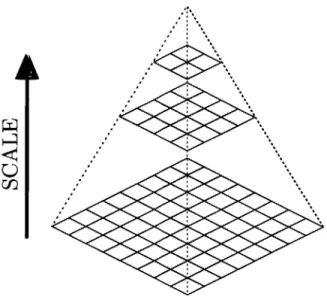
3.1 Multi-Scale Image Representations . . . . 3.2 The Octagonal Pyramid . . . .
9 . . . . 10 . . . . 12 . . . . 14 . . . . 15 . . . . 16 . . . . 17 . . . . 18 . . . . 19 21 . . . . 2 1 . . . . 26 . . . . 30 . . . . 30 . . . . 33 . . . . 36 . . . . 36 . . . . 40 45 46 51
3.2.1 Formulation . . . . 3.2.2 Directional Gradients . . . . 3.2.3 C olor . . . . 3.2.4 Computational Complexity . . . . 3.3 Considerations for Underwater Imagery . . . . . 3.3.1 Review of Underwater Image Formation 3.3.2 Illumination Invariance . . . . 3.3.3 Attenuation Invariance . . . . 3.4 Conclusions . . . .
4 Understanding Underwater Optical Image Datasets
4.1 Image Description . . . . 4.1.1 Keypoint Detection . . . . 4.1.2 Keypoint Description . . . . 4.1.3 Keypoint Detection With the Octagonal Pyramid . . . . 4.1.4 Description with QuAHOGs . . . . 4.2 Navigation Summaries . . . . 4.2.1 Clustering Data . . . . 4.2.2 Surprise-Based Online Summaries . . . . 4.2.3 Mission Summaries . . . . 4.3 Semantic Maps . . . . 4.3.1 Modified Navigation Summaries . . . . 4.3.2 Generating Semantic Maps . . . . 4.4 Conclusions . . . . 5 Discussion 5.1 Contributions . . . . 5.2 Future Work. . . . . . . . . 51 . . . . 56 . . . . 6 1 . . . . 64 . . . . 66 . . . . 67 . . . . 68 . . . . 70 . . . . 73 75 75 77 79 80 82 87 87 88 90 96 97 101 104 113 113 115
Chapter 1
Introduction
Seventy percent of the Earth's surface is covered by water, below which lie diverse ecosystems, rare geological formations, important archeological sites, and a wealth of natural resources. Understanding and quantifying these areas presents unique challenges for the robotic imaging platforms required to access such remote locations. Low-bandwidth acoustic communications prevent the transmission of images in real-time, while the large volumes of data collected often exceed the practical limits of exhaustive human analysis. As a result, the paradigm of underwater exploration has a high latency of understanding between the capture of image data and the time at which operators are able to gain a visual understanding of the survey environment.
While there have been advancements in automated classification algorithms, they rely on corrected imagery free of illumination and attenuation artifacts and are ill-suited to running on processor-limited robotic vehicles. The overarching contribution of this thesis is to reduce the latency of understanding by developing a lightweight framework for processing images in real time aboard robotic vehicles. Where correc-tion, classificacorrec-tion, and communication have previously been considered as separate problems, we consider them jointly in the context of invariant features and semantic compression.
1.1
Underwater Robotics
Underwater vehicles can be grouped into three main categories: Human Occupied Vehicles (HOVs) such as the well-recognized Alvin submersible [176]; Remotely Op-erated Vehicles (ROVs) such as Jason [8] or the towed HabCam system [164]; Au-tonomous Underwater Vehicles (AUVs) such as SeaBED [150] or REMUS [110]. Both HOVs and ROVs empower an operator with real-time data and visual feedback of the survey environment provided, in the case of ROVs, that the tether connecting the ROV to the surface ship has sufficient bandwidth [13]. AUVs, in contrast, are detached from the surface, allowing them to roam as far from a support ship as their batteries will permit while limiting the control and contact an operator has with the vehicle during a mission. Given these differences, AUVs will often be used as scouts to locate regions of interest that will later be surveyed by HOVs or ROVs [86]. While this thesis is primarily concerned with AUVs, much of the work can be applied to other robotic vehicles as well.
Terrestrial robots often rely on Global Positioning System (GPS) satellites for reliable localization, but these signals do not penetrate deep enough into the water column to be useful for navigation. Instead, underwater robots generally rely on an initial GPS fix at the surface and then estimate their location based on dead reckon-ing from on-board sensor measurements. AUVs carry a suite of navigational sensors including a magnetic compass, pressure sensors, acoustic altimeters, various attitude and rate sensors, and bottom-locking acoustic doppler sensors [88]. However, the position error grows unbounded in time without external inputs. A common method of bounding this error is to use a long baseline (LBL) network of stationary transpon-ders that are deployed from a ship and act like an underwater network of acoustic GPS beacons [177]. Ultra-short baseline (USBL) systems have been used for navi-gation as well as homing situations [3]. Other methods include remembering visual landmarks throughout the mission using optical [39] or acoustic [78] measurements. It is common for mapping sensors like cameras and multibeam sonars to have much higher resolutions than navigational sensors, so self-consistent maps have been
creat-ing from optical measurements [134], acoustic measurements [138], and from fuscreat-ing both together [91].
Without a physical link to the surface, AUVs rely on acoustic signals to com-municate with shipboard operators. These channels have very limited bandwidth with throughput on the order of tens of bytes per second depending on range, packet size, other uses of the channel (for instance, navigation sensors), and latencies due to the speed of sound in water [49, 159]. While much higher data rates have been achieved using underwater optical modems for vehicle control [32] and two-way com-munication [33], these systems are limited to ranges on the order of 100 meters and are inadequate for long-range communication [40]. In the absence of mission-time operator feedback, an AUV must either navigate along a preprogrammed course or use the data it collects to alter its behavior. Examples of the latter, termed adaptive mission planning, include detecting mines so potential targets can be re-surveyed in higher-resolution [50] and using chemical sensors to trace plumes back to their source [41, 77]. The overarching implication is that, with the exception of low-bandwidth status messages, data collected by an AUV is not seen by operators until after the mission is completed and the vehicle recovered.
Figure 1-1 compares the trends in computing power (quantified using processor cycles), hard disk storage, and underwater acoustic communication rates on a
log-arithmic scale over the past two decades. Hard disk storage space has followed an exponential increase in this time [61, 145, 30], while computing power followed a sim-ilar trend until the middle of last decade, where processor clock cycles leveled out around 3 GHz in favor of multi-threaded approaches [70, 127]. However, incoherent underwater acoustic communications in shallow and deep water at ranges of 1-10 kilo-meters, practical distances for AUV missions, have not increased their maximal bit rates over the past two decades [2, 49, 87, 115, 159]. Clearly, the ability to transmit data while underway has been and will remain a limiting factor in the AUV latency of understanding paradigm. While effective processing power continues to increase via parallelization, this comes at the price of additional power consumption. As disk capacity continues to increase and AUVs capture more and more imagery, there is an
10 5
Processor Cycles (Hz)
Hard Disk Storage (Bytes)
Acoustic Communications (bit/s)
1010-105
a
1990 1995 2000 2005 2010
Figure 1-1: Trends in computing power (black triangles), hard disk storage (blue circles), and incoherent underwater acoustic communication rates (red squares) on a logarithmic scale over the past two decades. Computing power has been quantified using clock cycles for various Intel processors based on their release dates. While com-puting and storage rates have increased, acoustic communication rates have remained relatively constant.
emerging need for efficient algorithms running on low-power processors that are capa-ble of distilling the vast amounts of collected image data into information summaries that can be transmitted through the bottleneck of the acoustic channel.
1.2
Underwater Imaging
We have better maps of the surface of Venus, Mars, and our moon than we do of the seafloor beneath Earth's oceans [156], primarily because, in many respects, the imagery is easier to obtain. Water is a strong attenuator of electromagnetic radia-tion [35], so while satellites can map entire planets from space using cameras and laser ranging, underwater vehicles must be within tens of meters at best for optical sensors to be useful. Mechanical waves do travel well through water, seen in how many animals have evolved the ability to visualize their surroundings using sound, but there is a tradeoff between source strength, frequency, and propagation distance. Ship-based sonars use lower frequencies to reach the bottom, but these longer
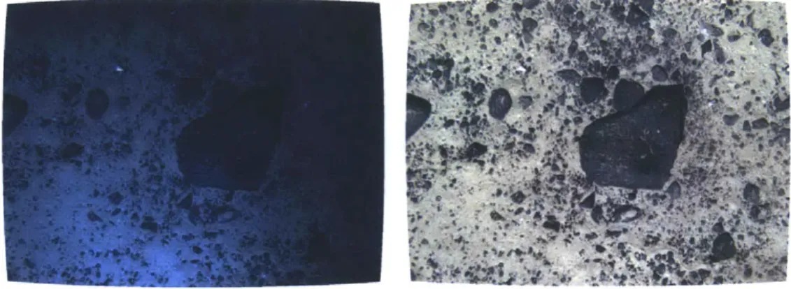
wave-Figure 1-2: Typical example of an underwater image captured by an AUV (left) and
after correction (right).
lengths come at the price of reduced resolution. To map fine-scale features relevant
to many practical applications, both optical and acoustic imaging platforms must
operate relatively close to the seafloor. This thesis focuses solely on optical imaging
because color and texture information are more useful for distinguishing habitats and
organisms, although some of the techniques presented in later chapters could be
ap-plied to acoustic imagery as well. Henceforth, when we refer to "underwater imagery"
we specifically mean optical imagery, in particular imagery which has been collected
by an AUV.
An underwater photograph not only captures the scene of interest, but is an image
of the water column as well. Attenuation of light underwater is caused by absorption,
a thermodynamic process that varies nonlinearly with wavelength, and by scattering,
a mechanical process where the light's direction is changed [35, 109]. Furthermore,
AUVs are often limited in the power they can provide for artificial lighting. As a
result, uncorrected underwater imagery is characterized by non-uniform illumination,
reduced contrast, and colors that are saturated in the green and blue channels, as
seen in Figure 1-2.
It is often desirable for an underwater image to appear as if it were taken in
air, either for aesthetics or as pre-processing for automated classification. Methods
range from purely post-processing techniques to novel hardware configurations, and
the choice depends heavily on the imaging system, the location, and the goals of the
photographer. For shallow, naturally-lit imagery, impressive results have been ob-tained using dehazing algorithms [22, 42] and polarizing filters [143]. For increasing greyscale contrast, homomorphic filtering [53, 148] and histogram equalization [147] are useful. In highly turbid environments, exotic lighting techniques have been em-ployed [59, 75, 73, 62, 95, 117]. For restoring color, methods range from simple white balancing [23, 113] to Markov Random Fields [167], fusion-based techniques [5], and even colored strobes [172]. In the case of many robotic imaging platforms, additional sensor information may be useful for correction as well [11, 15, 81, 85, 131, 137]. These topics are discussed in greater detail in the following chapter.
1.3
Image Understanding
Images provide a rich and repeatable means of remotely sampling an environment. Early examples of quantitative underwater imaging include diver-based camera quadrats
[31] and video transects [21] for mapping shallow coral reefs. Current AUV-based surveys are capable of generating orders of magnitude more image data [149, 133]. Manual methods for analyzing these datasets, such as using random points to assess percent cover [6, 31] or graphical user interfaces for species annotation [44, 164], are very labor intensive. Thus, there is a strong motivation to create algorithms capable of automatically analyzing underwater imagery.
The idea of what is "interesting" in an image is entirely guided by the opinions and goals of the observer. As a result, image processing is a diverse field boasting a wealth of literature in which selecting useful methods for applied problems relies heavily on heuristics. For the broad class of downward-looking underwater transect imagery, we can generalize two high-level goals: classifying the habitat and determining what
organisms exist there. These problems are commonly referred to in the literature as scene analysis and object detection, respectively.
1.3.1
Scene Analysis
Many scene identification problems have been addressed in the context of texture recognition [136], where texture can be quantified as both a statistical and structural phenomenon [64]. Arguably, a scene (habitat) is made up of objects (organisms), and if we abstract the idea of what these objects are, allowing them to be simple patterns, termed textons [82], the relative frequencies at which they occur can help identify the scene. This is known as a "Bag of Words" approach, which has its origins in document analysis based on the relative occurrences of key words.
The first step is to generate a vocabulary of textons. This can been done using a filter bank with kernels of assorted orientations, scales, and phases, as well as several isotropic filters [93]. Clustering the responses at each pixel using K-means or other clustering techniques, such as affinity propagation [51, 102], yields a dictionary of patterns that closely resemble image features such as bars and edges. Models of each texture are then learned as a histogram of textons across the image. Novel images can then be passed through the same filter bank, the responses quantized to the nearest texton, and the histogram compared to each model using the
X
2 distance [93] or other histogram metrics [102]. These filter banks were later made rotation invariant by only using the maximum response over several orientations [171]. Color textons have been proposed [16] although research suggests that texture and color should be dealt with separately [105].A drawback to the filter bank approaches is that they are relatively slow to com-pute. One solution to this is to directly use image patches, avoiding costly con-volutions [170]. These patches can be made more descriptive using an eigenmode decomposition or independent component analysis [102]. A disadvantage of patch-based methods is that they are not rotationally invariant. Proposed solutions to this involve finding the dominant patch orientation or training with patches at multiple orientations [170]. Experiments suggest that using dense grids rather than sparse keypoints for patch textons are better for scene classification [43].
a bottleneck at the quantization stage [169]. This overhead can be avoided by using a pre-defined and fast to compute set of textons, such as Local Binary Patterns (LBP) [121]. LBP works by comparing a central pixel to a constellation of neighbors at various scales and orientations. This comparison generates a binary code which is by definition contrast invariant and can be rapidly mapped to rotation invariant and more frequently-occurring patterns. Both patches [102] and LBP [158] have been successfully applied to underwater habitat classification.
In some cases, global histogram methods can be improved upon by taking into account spatial information as well. For instance, forests often have strong horizontal gradients from tree trunks while an image of a beach may have a narrow vertical gradient at the horizon. "GIST" features [122] concatenate histograms of gradient orientations over a coarse grid, similar to SIFT descriptors [104] but for an entire image. Pyramid match kernels [60] have been used to weight features more heavily that occur together at finer scales in similar locations [92]. However, these approaches are less useful for unstructured underwater imagery.
1.3.2
Object Detection
While many terrestrial object detection problems consist of "composed" imagery where the object is placed squarely in the camera field of view [128, 165], real-world objects or organisms are rarely so cooperative when photographed by an indiffer-ent robot. Furthermore, the role that context can play in aiding object recognition [123, 166], namely the co-occurrence of objects and scenes, is often the question a biologist is trying to answer, making it an unsuitable prior for classification. Still, modeling an object as a collection of parts can be useful. Keypoint descriptors like SIFT have been used with affine transformations to find identical objects in separate images [103]. However, this approach is ill-suited to biological variation in many or-ganisms. Quantizing those same keypoints and computing local histograms is similar to the texton approach [92, 151].
Multi-colored objects can be efficiently distinguished using color indexing [54, 163], effectively replacing a dictionary of textons with a palate of colors. This approach
is popular in content-based image retrieval (CBIR) paradigm [28, 155] because it in-volves easy to compute global features, is robust to clutter and occlusion, and the objects rough location can be recovered via histogram backprojection [163]. One drawback is that colors can change under different illumination conditions, so invari-ant color spaces have been explored as well [52].
In addition to general object detectors, there also exist many singular-class detec-tors as well. The use of coarse rectangular binned histograms of oriented gradients have been applied to human detection [27]. Integral images [173] have accelerated the detection of faces by approximating filter banks with box integrals. While detecting humans is a well-explored industrial-scale application, underwater organism detectors often employ even more specialized and heuristic approaches. Rockfish have been de-tected using a boosted three-stage detector based on color and shape [102]. Scallops have been detected using a blob detector followed by template matching [29] and by segmentation followed by color-based region agglomeration [164]. Coral reefs have been segmented and classified using features ranging from filter banks [79, 135], two-dimensional discrete cosine transforms [160], morphological features [84], and local binary patterns [157].
1.3.3
Machine Learning
Training an algorithm to recognize certain features based on manually labeled exam-ples is called supervised learning [4]. This can be useful both in post-mission analysis of underwater image transects [84, 102, 29] and in mainstream computer vision prob-lems like human detection [27, 173]. On the opposite end of the training spectrum,
unsupervised learning allows the computer to automatically select classes based on
trends in the data [4]. In fact, the generation of texton dictionaries via clustering [93, 171, 170] is an unsupervised learning step. This can be useful for understanding large underwater datasets of redundant imagery with several distinct scene classes [158] or for building online data summaries of a mission [55, 57, 125]. It should be noted that the computer does not attribute any semantic labels to the classes and all meaning is provided by human input. A hybrid between these two approaches is
semi-supervised learning [25] which seek to combine the relative strengths of
human-selected training labels with the pattern-finding abilities of computers. This latter approach could be particularly useful for reducing the time required to annotate datasets.
1.4
Communicating Visual Data
In almost all circumstances, the aspects of an image that are important to the user can be conveyed using many less bytes than are in the original image. This compressed image can then be transmitted more efficiently across a network using less bandwidth.
In lossless compression, the original image can be fully recovered from the compressed
format, where in lossy compression it cannot. Lossy compression techniques are ca-pable of higher compression rates than lossless techniques at the expense of making assumptions about what the user deems important. A common example of lossy compression is the JPEG format [175] which uses 8x8 blocks of the discrete cosine transform to achieve roughly 10:1 compression without major perceptual changes in the image. It is designed largely on models of human visual perception, so some of the artifacts make it ill-suited for image processing applications. A newer format, JPEG 2000 [154], employs variable compression rates using progressive encoding, meaning that a compressed image can be transmitted in pieces or packets that independently add finer detail to the received image. This is particularly well-suited to underwater applications where the acoustic channel is noisy and subject to high packet loss. How-ever, JPEG 2000 is optimized for larger packets that are unrealistic for underwater acoustic transmissions.
Recent work [112, 114] has focused on optimizing similar wavelet decomposition techniques for underwater applications using smaller packet sizes with set partitioning in hierarchical trees (SPIHT) [142]. These methods are capable of acoustically trans-mitting one 1024x1024 color image in under 15 minutes. Every 3 minutes the most re-cent image was compressed and queued for transmission, ensuring there would always be available imagery to transmit and providing the operator with a naive
understand-ing of the survey environment. Related work in online data summaries [55, 57, 125] focuses on determining a small subset of images that best represent a collection of images. At sub-image scales, saliency-based methods [80, 83] can recommend regions of interest within an image for preferential transmission.
In situations where image content is highly redundant, common in underwater image transects, image statistics can be compressed and transmitted in lieu of entire images, effectively communicating the content of the image. Images segmented into classification masks [114] have been compressed, transmitted, and then synthesized on the receiving end using any number of texture-synthesis techniques [38, 37, 97].
A similar scenario occurs in mobile visual search [58], a subset of the CBIR paradigm [28, 155], where a smart phone user wishes to perform a search based on the content of an image rather than tagged metadata. Rather than transmit the full-resolution image across the network, a collection of features is transmitted in its place. This has led to a transition away from traditional feature descriptors like SIFT [104] to compressed [24] or binary [20, 94, 141] descriptors that are faster to compute and require fewer bits to describe an image. A database indexed by these descriptors can be quickly searched and return results to the user.
1.5
Thesis Organization
The organization of this thesis is as follows. In Chapter 2, we derive a model of underwater image formation which we use in a detailed discussion of existing cor-rection techniques. We also present a novel corcor-rection method for robotic imaging platforms that utilizes additional sensor information to estimate environmental and system parameters. In Chapter 3, we develop a lightweight scale-space representation that reduces the complexity necessary to analyze imagery across multiple scales. We also demonstrate how this approach can be used to extract color and textural features that are invariant to underwater artifacts. In Chapter 4, we apply the framework of the previous chapter to real data collected by an AUV. We show how the latency of understanding can be reduced by transmitting both a subset of representative images
and classification masks learned through unsupervised techniques. In Chapter 5, we summarize our contributions and state potential directions for future work.
Chapter 2
Underwater Image Correction
This chapter describes the origin of underwater imaging artifacts and methods used to remove them. We first build a model of underwater image formation, describing how various artifacts arise. Next, we discuss a variety of common methods used to correct for these artifacts in the context of different modes of underwater imaging. Lastly, we present a novel method of correction for robotic imaging platforms that estimates environmental and system parameters using multi-sensor fusion.
2.1
Underwater Image Formation
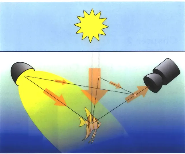
An underwater photograph not only captures the scene of interest, but is an image of the water column as well. Figure 2-1 diagrams a canonical underwater imaging setup. Light rays originating from the sun or an artificial source propagate through the water and reach the camera lens either by a direct path or by an indirect path through scattering. We deal with each of these effects in turn.
Attenuation
The power associated with a collimated beam of light is diminished exponentially as it passes through a medium in accordance with the Beer-Lambert Law
Figure 2-1: Capturing an underwater image. Light originating from the surface and/or an artificial source reflects off of an object (fish) and toward the camera along a direct path (solid line) or is scattered off of particles into the camera's field of view (dotted line).
where PO is the source power, P is the power at a distance f through the medium, A is wavelength, and a is the wavelength-dependent attenuation coefficient of the medium [35]. Attenuation is caused by absorption, a thermodynamic process that varies with wavelength, and by scattering, a mechanical process where the light's direction changes.
a(A) = aa(A) +
e,
(2.2)where aa(A) and a, are the medium absorption and scattering coefficients, respec-...
tively. Scattering underwater is largely wavelength-independent because the scatter-ing particle sizes are much larger than the wavelength of light. Underwater scenes generally appear bluish green as a direct result of water more strongly absorbing red light than other wavelengths. However, the attenuation properties of water vary greatly with location, depth, dissolved substances and organic matter [109].
Natural Lighting
Natural illumination E, from sunlight S, attenuates exponentially with depth z and can be characterized by R(A), the average spectral diffuse attenuation coefficient for spectral downwelling plane irradiance.
En(A, z) = Sn(A) e-(A)z (2.3)
While related to a, the diffuse attenuation coefficient represents the sum of all light arriving at a depth from infinitely many scattered paths. It is strongly correlated with phytoplankton chlorophyll concentrations and is often measured in remote sensing applications [109].
Artificial Lighting
At a certain depth, natural light is no longer sufficient for illumination, so artificial lights must be used. AUVs are generally limited in the amount of power they can pro-vide for lighting, so beam pattern artifacts are common. We can model the artificial illumination pattern Ea from a single source as
Ea(A) = Sa(A) BPo,oe 2 cos-y (2.4)
where Sa is the source spectrum, BPO,O is the angularly-dependent beam pattern intensity of the source, La is the path length between the source and the scene, and -y is the angle between the source and surface normal assuming a Lambertian surface [108]. In practice, imaging platforms may carry one or multiple light sources, but in our model we assume a single source for simplicity.
Diffuse Lighting
Light that is scattered back into the camera's line of sight is known as backscatter, a phenomenon similar to fog in the atmosphere [116]. If we denote F(A, z) to be the diffuse light field at any given point, we can recover the backscatter by integrating the attenuated field along a camera ray.
Eb(A) =
j
F(A, z)
ea(A)edf
(2.5)
Under the assumption that F(A, z) ~ F(A) is uniform over the scene depth f, then
Eb(A)
=A(A) (1
- e-(A)
(2.6)
where A(A) = F a(A) is known as the airlight. This additive light field reduces contrast and creates an ambiguity between scene depth and color saturation [42].
Camera Lens
The lens of the camera gathers light and focuses it onto the optical sensor. Larger lenses are preferable underwater because they are able to gather more light in an already light-limited environment. The lens effects L can be modeled as
D)2 (Z - FL
L = cos OL TL L (2-7)
2
Zs FL)
where D is the diameter of the lens, 6L is the angle from lens center, TL is the transmission of the lens, and Z. and FL are the distance to the scene and the focal length, respectively. Assuming there are no chromatic aberrations, the lens factors are wavelength-independent. A detailed treatment of this can be found in McGlamery and Jaffe's underwater imaging models [74, 108].
Optical Sensor
Since most color contrast is lost after several attenuation lengths, early underwater cameras only captured grayscale images. The intensity of a single-channel monochrome image c can be modeled as the integrated product of the spectral response function p of the sensor with incoming light field
c = JE(A)r(A)p(A) dA (2.8)
where E is the illuminant and r is the reflectance of the scene. Bold variables denote pixel-dependent terms in the image. Creating a color image requires sampling over multiple discrete spectral bands A, each with spectral response function PA. The human visual system does precisely this, using three types of cone-shaped cells in the retina that measure short (blue), medium (green), and long (red) wavelengths of light, known as the tristimulus response. Modern digital cameras have been modeled after human vision, with many employing a clever arrangement of red, green, and blue filters known as a Bayer pattern across the sensor pixels. This multiplexing of spatial information with spectral information must be dealt with in post-processing through a process called demosaicing, explained later in more detail.
A color image can be similarly modeled as
CA = JE(A)r(A)PA(A) dA ~ EArA. (2.9)
The illumant and reflectance can be aproximated in terms of the camera's red, green, and blue channels A ={R, G, B} with the understanding that they actually represent a spectrum [76]. By adjusting the relative gains of each channel, known as von Kries-Ives adaptation, one can transform any sensor's response into a common color space through simple linear algebra.
Imaging Model
Putting the pieces together, we arrive at a model with both multiplicative terms from the direct path and additive terms from the indirect scattered light field.
e-aAtes (
CA=
G
(En,A + Ea,A) rA £ + AA(1
-L
(2.10)G is an arbitrary camera gain. We ignore forward scattering from our model
because its contributions are insignificant for standard camera geometries [147].
2.2
Review of Correction Techniques
Removing the effects of the water column from underwater images is a challenging problem, and there is no single approach that will outperform all others in all cases. The choice of method depends heavily on the imaging system used, the goals of the photographer, and the location where they are shooting.
Imaging systems can range from a diver snapping tens of pictures with a hand-held camera to robotic platforms capturing tens of thousands of images. Where divers often rely on natural light, AUVs dive deeper and carry artificial lighting. AUVs gen-erally image the seafloor indiscriminately looking straight down from a set distance, while divers are specifically advised to avoid taking downward photographs and "get as close as possible" [36]. One individual may find enhanced colors to be more beau-tiful, while a scientist's research demands accurate representation of those colors. Similarly, a human annotating a dataset might benefit from variable knobs that can enhance different parts of the images, while a computer annotating a dataset demands consistency between corrected frames.
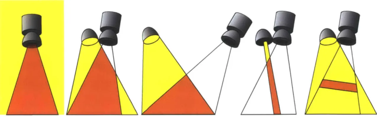
Lighting and camera geometry also play huge roles in the subsequent quality of underwater imagery. Figure 2-2 shows the effect that camera - light separation has on the additive backscatter component. Images captured over many attenuation lengths, such as a horizontally facing camera pointed towards the horizon, suffer more from backscatter than downward looking imagery captured from 1-2 attenuation lengths away. In many situations, the additive backscatter component can be ignored completely, while in highly turbid environments, exotic lighting methods may be required.
L
Figure 2-2: Backscatter is a direct result of the intersection (shown in orange) between
the illumination field (yellow) and the field of view of the camera. In ambient light
(far left) and when using a coincident source and camera (second from left) the entire
field of view is illuminated. Separating the source from the camera (middle) results
in a reduction of backscattering volume. Structured illumination (second from right)
and range gating (far right) drastically reduce the backscattering volume and are
ideal for highly turbid environments.
Shallow, Naturally Lit Imagery
Images captured in shallow water under natural illumination often contain a strong additive component. Assuming a pinhole camera model, image formation can be elegantly written as a matteing problem
CA= JA t +
(1
-t
)
AA
1
(2.11)
where JA = rA and t = e-"^a is the "transmission" through the water.
Dehazing algorithms [42, 22] are able to both estimate the color of the airlight and
provide a metric for range which are used to remove the effects of the airlight. Since
the scattering leads to depolarization of incident light, other methods employ
polar-izing filters to remove airlight effects
[143].
However, these methods do not attempt
to correct for any attenuation effects.
Enhancing Contrast
Several methods simply aim at enhancing the contrast that is lost through
atten-uation and scattering. Adaptive histogram equalization performs spatially varying
histogram equalization over image subregions to compensate for non-uniform illu-mination patterns in grayscale imagery [147]. Homomorphic methods work in the logarithmic domain, where multiplicative terms become linear. Assuming that the illumination field IA = (En,A + Ea,A) -0^4 contains lower spatial frequencies than the reflectance image, and ignoring (or previously having corrected for) any additive components,
log CA = log IA + log rA, (2.12)
the illumination component can be estimated though low-pass filtering [53] or surface fitting [148] and removed to recover the reflectance image. These methods work well for grayscale imagery, can be applied to single images, and do not require any a priori knowledge of the imaging setup. However, they can sometimes induce haloing around sharp intensity changes, and processing color channels separately can lead to misrepresentations of actual colors. Other contrast enhancement methods model the point spread function of the scattering medium and recover reflectance using the inverse transform [68].
High-Turbidity Environments
Some underwater environments have such high turbidity or require an altitude of so many attenuation lengths that the signal is completely lost in the backscatter. Several more "exotic" methods utilizing unique hardware solutions are diagrammed in Figure 2-2. Light striping [59, 62, 73, 117] and range gating [75] are both means of shrinking or eliminating, respectively, the volume of backscattering particles. Confocal imaging techniques have also been applied to see through foreground haze occlusions [95].
Restoring Color
The effects of attenuation can be modeled as a spatially varying linear transformation of the color coordinates
CA = IArA
(2.13)
where IA is the same illumination component defined in Equation 2.12. To recover the reflectance image, simply multiply by the inverse of the illumination component. Assuming that the illumination and attenuation IA ' IA are uniform across the
scene, this reduces to a simple white balance via the von Kries-Ives adaptation [76]. The white point can be set as the image mean under the grey world assumption, a manually selected white patch, or as the color of one of the brightest points in the image [23, 113]. This method achieves good results for some underwater images, but performs poorly for scenes with high structure. Results can also be negatively affected when the grey world assumption is violated, for instance a large red object which shifts the mean color of the image. Recent work in spatially varying white balance [69] would be interesting to apply to underwater images as well.
More computationally involved methods include fusion-based approaches that combine the "best" result of multiple methods for color correction and contrast en-hancement [5]. Markov Random Fields have been used with statistical priors learnt from training images to restore color [167]. A novel hardware solution to restoring color employs colored strobes to replace the wavelengths lost via attenuation [172].
Beyond a Single Image
Additional information beyond that contained in a single image can be useful for correcting an image. The simplest method is to compute the average across many image frames
K 1K
K
ZCA,k
IAK 7A,k
= IArA(2.14)
k k
under the assumption that the illumination component does not vary between images. This assumption is valid for many types of robotic surveys where a constant altitude is maintained over a relatively uniform seafloor [81, 131]. Correction is then akin to that of a spatially varying white balance where the white point of each pixel
is the mean over the dataset.
Robotic platforms often carry additional sensors other than a single camera and light source. An acoustic altimeter can provide information to perform range-dependent frame averaging useful for towed systems where a constant altitude is difficult to main-tain [137]. However, this approach fails when the bottom is not flat relative to the imaging platform. Multiple acoustic ranges, such as those obtained from a Doppler Velocity Log (DVL), can be used under the assumption that the bottom is locally planar [85]. Stereo camera pairs [15] or a sheet laser in the camera's field of view [11] can similarly provide bathymetry information for modeling attenuation path lengths.
2.3
Correction for Robotic Imaging Platforms
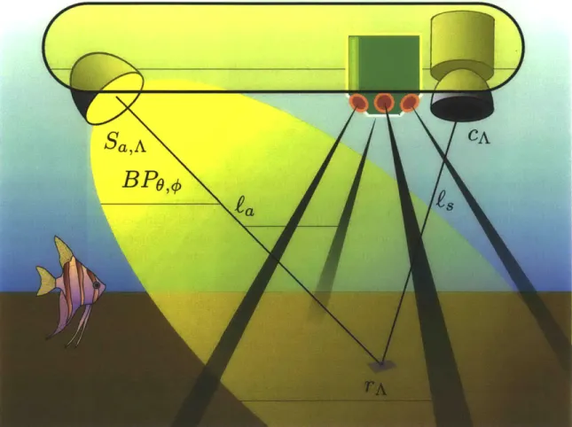
In addition to cameras and artificial light sources, robotic imaging platforms generally carry a suite of navigational sensors as well. One such sensor in widespread use is the Dopper Velocity Log (DVL) which measures both range and relative velocity to the seafloor using 4 acoustic beams [1]. Figure 2-3 diagrams a common configuration for many robotic imaging platforms. The camera and light source are separated to reduce backscatter, and the DVL is mounted adjacent to the camera so its beams encompass the field of view. Unlike many correction methods for single images that rely on assumptions such as low frequency illumination patterns, we exploit multiple images and additional sensor information to estimate the unknown parameters of the imaging model and use this to obtain more consistent image correction.
2.3.1
Assumptions
We first assume that our images are captured deep enough so that natural light is negligible relative to artificial lighting. We also assume there is a single strobe, and its spectrum SA ~{1, 1, 1} is approximately white. This is an acceptable assumption because, while deviations in the strobe spectrum will induce a hue shift in the cor-rected reflectance image, this shift will be constant over all images in a dataset. Thus, even a strongly colored strobe would have no effect on automated classification results
Figure 2-3: Diagram of a robotic imaging platform. The camera and light are
sep-arated to reduce backscatter, and a DVL is mounted adjacent to the camera so its
beams encompass the field of view.
0 810 12
2 4 A 6itd (m8 10 12
Figure 2-4: Log color channel means (colored respectively) for over 3000 images captured along a transect as a function of altitude. Note the linearity within the first few meters, suggesting that additive effects can be ignored. Diffuse lighting dominates at higher altitudes, asymptotically approaching the airlight color. The falloff at very low altitudes is due to the strobe beam leaving the camera's field of view.
assuming the training and testing were both performed with corrected imagery. Next, we assume that we can ignore the additive effects of scattered diffuse light-ing. This is a valid assumption for images captured in relatively clear water within a few meters of the seafloor, as demonstrated in Figure 2-4. The log of each color channel mean for 3000 images has been plotted as a function of vehicle altitude over the course of a mission. At high altitudes, diffuse light from the scattered illumination field dominates, asymptotically approaching the airlight color. Within the first few meters, however, the relationship is roughly linear, indicating the relative absence of additive scattering effects.
Neglecting additive components allows us to work in the logarithmic domain, where our image formation model becomes a linear combination of terms. Approxi-mating the seafloor as a locally planar surface, we can neglect the Lambertian term cos'y as it will vary little over the image. The gain G and lens
L
terms are constantbetween images and effect only the brightness but not the color. Omitting them as well, our model reduces to
log CA = log rA + log BPo,o - OaA(ea + ,) - 2log ae. (2.15) From this we can clearly see three processes corrupting our underwater image. Firstly, the beam pattern of the strobe creates a non-uniform intensity pattern across the image as a function of beam angles 0 and
#.
Second is attenuation, which is wavelength-dependent and directly proportional to the total path length e = La + 4,. Lastly, there is spherical spreading, which in practice we have found to be less significant than the exponential attenuation, supported by [47], and henceforth omit from our calculations.At the moment, the entire right hand side of Equation 2.15 consists of unknowns. However, using the 4 range values from the DVL, and with a priori knowledge of offsets between sensors, we can fit a least squares local plane to the seafloor and compute the values of e, 6, and
4
for each pixel in the image. Although the vast majority of DVL pings result in 4 usable ranges, sometimes there are unreturned pings. In the case of three pings, a least squares fit reduces to the exact solution. For one or two returns, the bottom is simply assumed to be flat, although these cases are rare.This computation also requires that the projected ray direction in space is known for each pixel. Because the refractive index of water differs from that of air, the camera lens must be calibrated to account for distortion using the method described in [67]. An example of this rectification process is shown in Figure 2-5.
2.3.2
Attenuation Coefficient Estimation
For the moment, let us assume that the beam pattern BP,0 ~ 1 is uniform across the image. For each pixel in each color channel, we have one equation but 2 unknowns: the attenuation coefficient cA and the reflectance value rA that we are trying to re-cover. However, if that same point is imaged from another pose with a different path
Figure 2-5: Original image (left) rectified for lens distortion (right).
length, an equation is added and the system can be constrained. For the purposes of navigation and creating photomosaics, finding shared features between overlapping images is a common problem. Keypoints can be reliably detected and uniquely de-scribed using methods such as Harris corners and Zernike moments [131] or SIFT features [118]. An example of two overlapping images with matched keypoints is shown in Figure 2-6.
For each pair of matched keypoints, the average local color value is computed using a Gaussian with standard deviation proportional to the scale of the keypoint. As-suming that the corrected values of both colors should be the same, we can explicitly solve for the attenuation coefficients
log cA,1 -logcA,2
(2.16)
2 f~l$
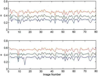
The mean values of CeA were calculated for each of 100 images. Values less than
0.1 were considered unrealistic and omitted. This accounted for 20% of the images. The results are plotted at the top of Figure 2-7.
This method is feasible for as few as two images assuming that there is overlap between them and enough structure present to ensure reliable keypoint detection, which is usually not an issue for AUV missions. For towed systems, however, alti-tude and speed are more difficult to control, so we propose a second simpler method for estimating the attenuation coefficients. Figure 2-4 plotted the log color channel means over a range of altitudes. For altitudes between 1-5 meters, the relationship is
Figure 2-6: A pair of overlapping images with matched keypoints. 0.6 ts 0.4 0 ) 10 20 30 40 50 60 70 80 0 10 20 30 40 Image Number 50 60 70 80
Figure 2-7: Estimated aA, color coded respectively, for uncorrected images (top) and
beam pattern corrected images (bottom). Values less than 0.1 have been ignored.
Dotted lines are mean values. Note how well the triplets correlate with each other,
suggesting that the variation in the estimate originates from brightness variations
between images.
0.8 0.6 t 0.4 0.2 A si 1, IN 111% ''11jQ I I o''k V1-1 0.2roughly linear, which we used to justify ignoring any additive scattering in our model. Assuming that the average path length ~ 2a is approximately twice the altitude, then the attenuation coefficients can also be estimated as half the slope of this plot.
2.3.3
Beam Pattern Estimation
While the strobe's beam pattern induces non-uniform illumination patterns across images, this beam pattern will remain constant within the angular space of the strobe. Assuming a planar bottom, each image represents a slice through that space, and we are able to parameterize each pixel in terms of the beam angles 0 and q. If we consider only the pixels p E
[Oi,
#j]
that fall within an angular bin, the average intensity value corrected for attenuation will be a relative estimate of the beam pattern in that direction.log BP(Oi, #j) =
CA +loc
a -Ae (2.17)A 1 P
Assuming that there is no spatial bias in image intensity (for instance the left half of the images always contain sand and the right half of the images only contain rocks) then the reflectance term only contributes a uniform gain. This gain is removed when the beam pattern is normalized over angular space. The resulting beam pattern is shown in Figure 2-8.
We also recompute the attenuation coefficients using color values for the beam pattern corrected imagery. The results are shown in the bottom of Figure 2-7. The triplets correlate quite well with each other, suggesting that variation in the estimates arises from intensity variation between images and not necessarily within images.
2.3.4
Image Correction
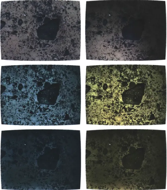
Each captured image can be corrected by multiplication with the inverse of the beam pattern and attenuation terms. Figure 2-9 shows different levels of correction. The top right image has been corrected for attenuation alone, and while its colors look more realistic there is still a strong non-uniform illumination present. The bottom
3 0 2 2 -10 0 10 20 30 Degrees Starboard
Figure 2-8: Estimated beam pattern of the strobe in angular space. Warmer hues indicate higher intensities, while the dark blue border is outside the camera field of view. Axes units are in degrees, with (0,0) corresponding to the nadir of the strobe. The strobe was mounted facing forward with a downward angle of approximately 70 degrees from horizontal. The camera was mounted forward and starboard of the strobe. Note how the beam pattern is readily visible in figure 2-9.
Figure 2-9: Original image (top left) corrected for attenuation alone (top right), beam
pattern alone (bottom left), and both (bottom right).
left image has been corrected for beam pattern alone, and thus maintains a bluish
hue from attenuation. The bottom right image has been corrected for both artifacts.
Figure 2-10 shows some other methods of correction. In the upper right frame,
white balancing achieves similar results to correction for attenuation alone with the
beam pattern still present. In the lower 2 images in the left column, adaptive
his-togram equalization and homomorphic filtering have been applied to the intensity
channel of each image. While the beam pattern has been eliminated, haloing
arti-facts have been introduced around sharp contrast boundaries in both images. To the
right, white balancing each of these produce aesthetically pleasing but less realistic
results. In the upper left, frame averaging returns the most realistic-looking image
whose colors compare well to our results.
The artifacts of attenuation and illumination are sometimes hidden when
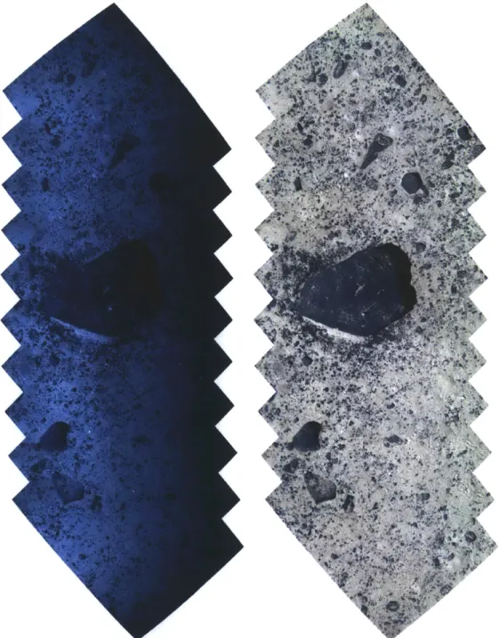
photo-mosaics are created and images blurred together. Figure 2-11 shows photomosaic of
Figure 2-10: Example methods of correction methods applied to the original image
in Figure 2-9. Frame averaging (top left). White balancing (WB) with grey-world
assumption (top right). Adaptive histogram equalization (AHE) (middle left). AHE
with WB (middle right). Homomorphic filtering (bottom left). Homomorphic filtering
with WB (bottom right). Note how each image is aesthetically more pleasing than
the original raw image, but there is significant variation between each method.
the same area before and after correction. While much of the along-track variation in illumination has been blurred away, there is still a definitive difference in brightness in the across-track direction.
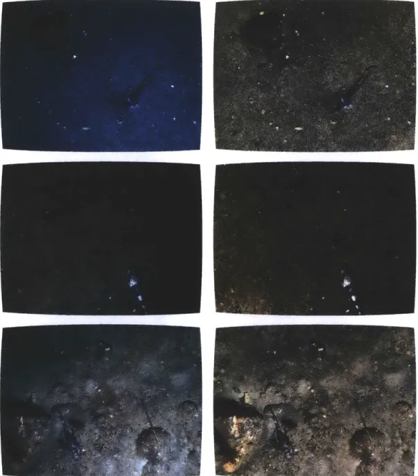
Several more pairs of raw and corrected images are shown in Figures 12 and 2-13. These images were captured at various benthic locations between the Marguerite Bay slope off the western Antarctic Peninsula and the Amundsen Sea polynia. While the same beam pattern estimates are used for all images, the value of the attenua-tion coefficients varied enough between locaattenua-tions that using mismatched coefficients produced unrealistic looking results. While correlating attenuation with parameters such as salinity or biological activity is beyond the scope of this thesis, it presents interesting topics for future research into measuring environmental variables using imagery.
2.4
Conclusions
In this chapter, we have derived an underwater image formation model, discussed a diverse assortment of methods used to obtain and correct high-quality underwater images, and presented a novel method for corrected underwater images captured from a broad family of robotic platforms. In this method, we use acoustic ranges to constrain a strong physical model where we build explicit models of attenuation and the beam pattern from the images themselves. Our goal was never to develop a unifying method of correction, but rather to emphasize a unified understanding in how correction methods should be applied in different imaging situations.
Because robotic platforms generate datasets that are often too large for exhaus-tive human analysis, the emphasis on their correction should involve batch methods that provide consistent, if not perfectly accurate, representations of color and tex-ture. Available information from other onboard sensors can and should be utilized to improve results. An unfortunate side effect of this is that correction techniques tend to become somewhat platform-specific. However, it is not surprising that more realistic correction is obtained when all available information is taken into account.
Figure 2-11: Raw (left) and corrected (right) photomosaics from a sequence of 10
images. Note how the non-uniform illumination pattern is blurred between frames in
the left image.
Furthermore, we re-emphasize that a corrected image alongside a raw image con-tains information regarding the water column properties, the bottom topography, and the illumination source. Given this residual, any correction scheme will naturally provide insight to some projection of these values in parameter space. In the absense of ground truthing, which is often unrealistic to obtain during real-world mission sce-narios, one possible metric is to compare methods based on their residual, or what they estimate the artifacts to be, for which approach most closely approximates the physical imaging situation. While this metric is somewhat contrived, it is apparent that the approach which best estimates this residual will also provide superior results.