Statistical analysis on spatial correlation of ionospheric day-to-day variability by using GPS and Incoherent Scatter Radar observations

HAL Id: hal-00318367

https://hal.archives-ouvertes.fr/hal-00318367

Submitted on 29 Aug 2007

HAL is a multi-disciplinary open access

archive for the deposit and dissemination of

sci-entific research documents, whether they are

pub-lished or not. The documents may come from

teaching and research institutions in France or

abroad, or from public or private research centers.

L’archive ouverte pluridisciplinaire HAL, est

destinée au dépôt et à la diffusion de documents

scientifiques de niveau recherche, publiés ou non,

émanant des établissements d’enseignement et de

recherche français ou étrangers, des laboratoires

publics ou privés.

day-to-day variability by using GPS and Incoherent

Scatter Radar observations

X. Yue, W. Wan, L. Liu, T. Mao

To cite this version:

X. Yue, W. Wan, L. Liu, T. Mao. Statistical analysis on spatial correlation of ionospheric day-to-day

variability by using GPS and Incoherent Scatter Radar observations. Annales Geophysicae, European

Geosciences Union, 2007, 25 (8), pp.1815-1825. �hal-00318367�

Ann. Geophys., 25, 1815–1825, 2007 www.ann-geophys.net/25/1815/2007/ © European Geosciences Union 2007

Annales

Geophysicae

Statistical analysis on spatial correlation of ionospheric day-to-day

variability by using GPS and Incoherent Scatter Radar observations

1_{Institute of Geology and Geophysics, Chinese Academy of Sciences, Beijing 100029, China} 2_{Wuhan Institute of Physics and Mathematics, Chinese Academy of Sciences, Wuhan 430071, China} 3_{Graduate School, Chinese Academy of Sciences, Beijing 100049, China}

Received: 22 March 2007 – Revised: 12 July 2007 – Accepted: 3 August 2007 – Published: 29 August 2007

Abstract. In this paper, the spatial correlations of

iono-spheric day-to-day variability are investigated by statistical analysis on GPS and Incoherent Scatter Radar observations. The meridional correlations show significant (>0.8) correla-tions in the latitudinal blocks of about 6 degrees size on av-erage. Relative larger correlations of TEC’s day-to-day vari-abilities can be found between magnetic conjugate points, which may be due to the geomagnetic conjugacy of several factors for the ionospheric day-to-day variability. The cor-relation coefficients between geomagnetic conjugate points have an obvious decrease around the sunrise and sunset time at the upper latitude (60◦_{) and their values are bigger} be-tween the winter and summer hemisphere than bebe-tween the spring and autumn hemisphere. The time delay of sunrise (sunset) between magnetic conjugate points with a high dip latitude is a probable reason. Obvious latitude and local time variations of meridional correlation distance, latitude varia-tions of zonal correlation distance, and altitude and local time variations of vertical correlation distance are detected. Fur-thermore, there are evident seasonal variations of meridional correlation distance at higher latitudes in the Northern Hemi-sphere and local time variations of zonal correlation distance at higher latitudes in the Southern Hemisphere. These vari-ations can generally be interpreted by the varivari-ations of con-trolling factors, which may have different spatial scales. The influences of the occurrence of ionospheric storms could not be ignored. Further modeling and data analysis are needed to address this problem. We suggest that our results are useful in the specific modeling/forecasting of ionospheric variabil-ity and the constructing of a background covariance matrix in ionospheric data assimilation.

Keywords. Ionosphere (Ionospheric disturbances;

Model-ing and forecastModel-ing, Solar radiation and cosmic ray effects)

Correspondence to: W. Wan (wanw@mail.iggcas.ac.cn)

1 Introduction

It is now well known that the ionosphere displays both a background state (climatology) and a disturbed state (weather). These variations cover a wide range of time scales, which range from operational time scales of hours and days up to solar cycles and even long-term trends (Rish-beth, 1998). Among these variabilities with different time scales, day-to-day variability is one of the most frequently in-vestigated recently for both scientific and applicable reasons (Forbes et al., 2000; Fuller-Rowell et al., 2000; Mendillo et al., 2002; Rishbeth and Mendillo, 2001). Bradley et al. (2002) have given a detailed explanation of the terminol-ogy variability. Most of the ionospheric characteristic pa-rameters’ day-to-day variability, including foF2, hmF2, foF1, foE, B0, and B1, have been studied by using ionosonde ob-servations from single, regional, or global stations (Dabas et al., 2006; Araujo-Pradere et al., 2005; Fotiadis and Kouris, 2006). This research give us a general variation of iono-spheric variability versus solar radiation, geomagnetic ac-tivity, latitude, and local time. Furthermore, Bradley et al. (2004) and Miro Amarante et al. (2004) even investigated the day-to-day variability of electron density profiles. Ex-cept for statistical analysis, Fuller-Rowell et al. (2000) and Mendillo et al. (2002) have modeled the ionospheric vari-ability response to geomagnetic activity and meteorological disturbances quantitatively, using different theoretical mod-els, respectively.

However, most research related to day-to-day variability in the past concentrated on its variations with local time, latitude, solar and geomagnetic activity, and attempted to give corresponding physical explanations. The spatial cor-relation scales of these variabilities have rarely been investi-gated systematically (at least to our knowledge up to now), except for Bradley et al. (2004), who have investigated the correlations of the variabilities of different parameters. The spatial correlation is a measure of how well a deviation at

one point is mirrored at a remote point. Perfectly corre-lated data will have correlation coefficients equal to 1, drop-ping to 0 for no correlation between the data, and -1 for perfect anti-correlation. The horizontal correlation of iono-spheric climatology has been studied by several researchers using ionosonde, GPS, and TOPEX observations (Bust et al., 2001; Gail et al., 1993; Huang, 1983; Klobuchar et al., 1995; Nisbet et al., 1981; Rush, 1976; Saito, 1978). But most of these papers investigated the horizontal correlation of the mid-latitude area. Few investigations are related to the ionospheric vertical correlation. Furthermore, the spatial correlation of different time scales in ionosphere may have differences, as they have different causes. Yu et al. (2007) have investigated the correlation distance of NmF2’s day-to-day variability by using ionosonde observations in Eu-rope. But their conclusions can only be applied to the mid-latitude. In this paper, we will investigate the spatial cor-relation including both the horizontal and vertical correla-tion of ionospheric day-to-day variability systematically by statistical analysis on GPS and Incoherent Scatter Radar ob-servations on a global scale. There are also several other reasons for us to implement this work as follows. (1) Iono-spheric weather can have detrimental effects on several hu-man activities and systems, including high-frequency com-munications, over-the-horizon radars, and survey and navi-gation systems using Global Positioning System (GPS) satel-lites. To avoid the destructive effects of ionosphere weather on military and civilian systems, there is a growing need to more accurately represent and forecast the ionosphere. Ac-cording to Nisbet et al. (1981), it would be necessary to in-clude some measure of the ionosphere’s day-to-day variabil-ity to obtain a more accurate prediction of the ionosphere. They found that the data within 1000 km of the point to be predicted were useful for the prediction. Beyond 3000 km the accuracy of the updated model was found to be no better than the predictions made using the model alone. Actually, here the 1000 km or 3000 km is related to the spatial corre-lation distance of the ionosphere. So it is important for us to know exactly the variation of the ionospheric spatial cor-relation of day-to-day variability versus many factors, such as latitude and local time, to give a more accurate predic-tion of ionospheric weather. Furthermore, the scale factor (SF), which is frequently used in ionosphere mapping, is also correlated with the ratio of zonal correlation distance to the meridional correlation distance (Stanislawska et al., 1996). (2) Recently, many researchers attempt to incorpo-rate observations and ionospheric models by using optimiza-tion schemes, known as the data assimilaoptimiza-tion method, to give specific representation of the ionosphere (Bust et al., 2004; Fuller-Rowell et al., 2006). When doing the data assimila-tion, especially based on the empirical model, an accurate correlation model of the ionosphere is very important (Bust et al., 2004; Fuller-Rowell et al., 2006). It determines the extent of data influence on regions where there is no data. (3) According to Rishbeth and Mendillo (2001), there are

many causes that can result in the day-to-day variability of the ionosphere. A better knowing of the ionospheric correla-tion distance of these variabilities may help us to understand the spatial scale of different causes.

The remainder of this paper is organized as follows. Sec-tion 2 describes the data source and analysis method. The results are given in Sect. 3. We give our discussions and con-clusions in Sects. 4 and 5.

2 Data source and analysis method descriptions

In this paper, we assume that the spatial correlations of the ionosphere are separable meridionally, zonally and vertically, as Bust et al. (2004) did. We use GPS-TEC to investi-gate the horizontal correlation of the ionosphere. The TEC value used here is the Jet Propulsion Laboratory Global Iono-spheric Map (JPL GIM). Mannucci et al. (1998) and Iijima et al. (1999) have described the method and process of retriev-ing the grid vertical TEC from global GPS measurements in detail. They used the Kalman filter to simultaneously solve for the values of hardware biases and the vertical TEC map. From the many IGS stations available, up to 100 stations are selected to optimize geographic coverage. With the increase in the number of IGS stations, the selected stations are not fixed. So we could not show the exact GPS stations used here. The vertical TEC data provided are between geograph-ical latitude –87.5◦ _{and 87.5}◦_{with an interval of 2.5}◦_{, and} between geographical longitude –180◦_{and 180}◦_{with an} in-terval of 5◦_{. As we know, the ionospheric electron density} is more symmetrical in geomagnetic coordinates than in ge-ographical coordinates. So we first transform the data in a geographical reference frame to apex magnetic coordinates by interpolation (Richmond, 1995). According to Mannucci et al. (1998), the GIM products have relatively larger errors in high latitudes and ocean areas because of less coverage. So we just used the data between the apex magnetic latitude –60◦_{and 60}◦_{. It should be pointed out that GIM data errors} associated with the thin spherical shell assumption, the data interpolation, and the insufficient station coverage in ocean areas, may affect the statistical results. By comparison with TOPEX TEC, the daily RMS accuracy of GIM TEC maps has been better than 10 TECU. Accuracy has been better than 5 TECU in the months where the TEC was low (Iijima et al., 1999). But the error may be smaller inland because of better data coverage there.

The Millstone Hill (42.6◦_{N, 288.5}◦_{E; 72}◦_{N Dip)} Inco-herent Scatter Radar observed electron densities from 4 Oc-tober to 4 November 2002, are used to study the vertical correlation of the ionosphere. The profiles are fitted by the two-layer Chapman function (Fox, 1994). The fit method used here is focused on the F2-layer. So it may have a rela-tively bad performance when the profile in the topside iono-sphere demonstrates an inflection point or a second peak or when the F1 layer exists (Fox, 1994). Then we calculate the

X. Yue et al.: Statistical analysis on spatial correlation of ionosphere 1817

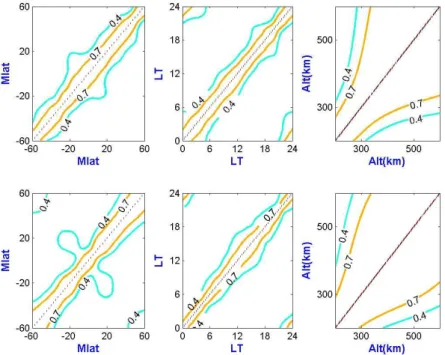
Fig. 1. Correlation coefficients’ sketch map. From left to right panels are meridional, zonal, and vertical correlation coefficients, respectively. Meridional correlation coefficients are shown between mlat –60◦_–60◦_{, and the top and bottom panel corresponds to night and day time. Zonal}

correlation coefficients are shown between different local times, and the top and bottom panels are for mlat 40◦_{and 0}◦_{, respectively. Vertical}

correlation coefficients are shown between 200–600 km, and the top and bottom panels are for night and day time, respectively.

electron densities between 200–600 km with an interval of 2 km by the fitted coefficients.

To calculate the correlations of N variables in a vector ϕ, we first construct a matrix consisting of different samples of ϕ. Then the variance covariance matrix of the sample matrix is obtained. The correlation coefficient can then be calculated from the covariance element. The processes are represented by the equations: A = (ϕ1, ϕ2, ..., ϕm) ∈ RN ×m A′_{= A − A} P = A_m−1′(A′)T Rij = √_PPij iiPjj , (1)

where A is the sample matrix of vector ϕ, A is the sample mean of A, P is the variance covariance matrix of A, and Rij is the correlation coefficient between variables i and j in vector ϕ. The correlation coefficients of electron densities are derived as follows. At first, the day-to-day variabilities of TEC and electron densities are calculated by differenc-ing them with their corresponddifferenc-ing value from the previous day. For TEC, we chose the data of 2000 and 2005 to repre-sent high and low solar activities, respectively. According to Araujo-Pradere et al. (2004), it may be useful to introduce in-termediate seasons between winter or summer solstices and the equinox, in the seasonal variation analysis of the iono-spheric variability. But in our work, the statistical results de-pend on the sample numbers. The addition of a season means

relativly less days in each season. So the data are divided into four samples, which correspond to the interval of February– April, May–July, August–October, and November–January, respectively, in every year in this work. The horizontal cor-relations are calculated for the eight samples, respectively, to investigate their solar and season variations. But for vertical correlations, only one sample is used here. The longitudi-nal effects are ignored when calculating both meridiolongitudi-nal and zonal correlations. Then the correlation coefficients are ob-tained for the three directions, respectively.

3 Results

3.1 Correlation coefficients’ sketch map

Typical correlation coefficients of three directions are shown in Fig. 1. According to the figure, both meridional and verti-cal correlations have differences between day time and night. The meridional correlations show significant (>0.8) correla-tion in the latitudinal blocks of about 6 degrees on average. Relatively larger correlations can be found between the mag-netic conjugate points. Furthermore, the vertical correlation has obvious altitude dependence. In the following, we will give detailed results about these variations of the correla-tions versus different factors, including local time, latitude, altitude, and season.

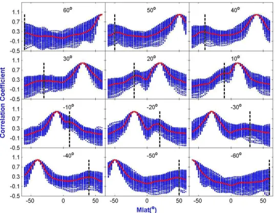
Fig. 2. (a) Correlation coefficients between one fixed apex latitude with all other apex latitudes from –60◦_{to 60}◦_{. The number in every}

subplot is the corresponding apex latitude. The solid lines are mean values of different local time, month and year. The vertical dashed lines mark the corresponding magnetic conjugate latitude.

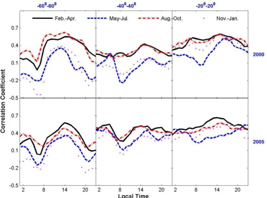
3.2 Correlation between magnetic conjugate points Before illustrating the correlation coefficients results, it is important for us to know exactly which level of correlation coefficient is significant or strong. As Bradley et al. (2004) said, there is no consensus as to what represents significant or a highly significant correlation, with some arguing that there is only interest in occasions with R>0.9. In this pa-per, we will follow their opinion and do not say significant when the correlation coefficient is less than 0.9. Relatively larger correlations can be found between magnetic conjugate points from the isoline map of meridional correlation, espe-cially during the daytime. Figure 2a shows the correlation coefficients between one fixed apex latitude with all other apex latitudes from –60◦_{to 60}◦_{. The number in every} sub-plot is the corresponding apex latitude. The solid lines are mean values of different local time, month and year. The ver-tical dashed lines mark the corresponding magnetic conju-gate latitude. The correlation coefficients between one fixed apex latitude and the field near its conjugate latitude have obvious protuberance. Figure 2b shows the local time vari-ations of the correlation coefficients between magnetic con-jugate points during the interval of February–April, May– July, August–October, and November–January, respectively. With the increase in latitude, the local time variations

be-come more evident. The correlation coefficients between – 60◦ _{and 60}◦ _{have an obvious decrease in sunrise and} sun-set time. During the interval of May–July and November– January, even negative correlations can be found between – 60◦_{and 60}◦_{near sunrise and sunset. In the main, the} corre-lation coefficients between conjugate points are bigger dur-ing the interval of February–April and August–October than May–July and November–January, which means the correla-tions between conjugate points are greater in the equinoxes than in the solstices.

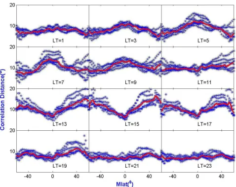
3.3 Meridional correlation distance

In this paper, the correlation distance is defined as the separa-tion at which the correlasepara-tion coefficient falls to 0.75. The hor-izontal and vertical correlation distances are represented by degree and kilometer, respectively. The latitude, local time, and seasonal variations of the meridional correlation distance are shown in Fig. 3. According to the figure, we can obtain several conclusions. There are no evident latitude variations of the meridional correlation distance around midnight. The mean value is between 7◦_{and 8}◦_{. In the daytime, the} merid-ional correlation distance is bigger in the mid-latitude than in the low and equatorial latitudes and the value varies from 10◦ _{in mid-latitude to 5}◦ _{in the equatorial area. However,}

X. Yue et al.: Statistical analysis on spatial correlation of ionosphere 1819

Fig. 2. (b) Local time variations of the correlation coefficients between magnetic conjugate points for the interval of February–April (solid lines), May–July (dashed lines), August–October(dashdot lines), and November–January (dots), respectively. The panels from left to right are for the magnetic conjugate points –60◦_–60◦_{, –40}◦_–40◦_{, –20}◦_–20◦_{, respectively. The top panel is the situation of year 2000, while the}

bottom for 2005.

around sunrise (from LT=3 to LT=9), the meridional correla-tion distance is larger in the equatorial area than in the mid-latitude, whose mean value varies from 11◦ _{to 5}◦_{. For all} the selected latitudes, the meridional correlation distance is larger in the daytime than in the nighttime, which is consis-tent with that of Yu et al. (2007). The mean value is between 5◦ _{and 15}◦_{. Except for areas around the equator (from –} 20◦_{to 20}◦_{), where the max meridional correlation distance} of a day appears around sunrise, the maximum always arises in the afternoon (around LT=14). In the mid-latitude of the Northern Hemisphere (from 40◦_{to 60}◦_{), the meridional} cor-relation distance is larger in summer than in equinox and larger in equinox than in winter. Yu et al. (2007) also ob-tained the same seasonal variations from ionosonde observa-tions in Europe. But for the rest of the latitudes, no obvious season variations can be found.

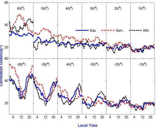
3.4 Zonal correlation distance

In this paper, the zonal correlation distance is defined as the east-west separation at which the correlation coefficients falls to 0.75. Local time variations of the zonal correlation dis-tance for the selected latitudes during different seasons are shown in Fig. 4. It is seen that the zonal correlation distance increases with the increase in latitude in both hemispheres.

The mean value varies from 40◦ _{in the mid-latitude} (abso-lute latitude is equal to 60◦_{)to 20}◦ _{in the equator. Except} in the mid-latitude of the South Hemisphere (between –60◦ and –40◦_{), where the zonal correlation distance is larger in} the nightside than in the dayside, there are no distinct local time variations in the rest area. The same holds true for the zonal correlation distance as meridional correlation distance; the zonal correlation distance is little larger in summer than in the other seasons in the mid-latitude of the North Hemi-sphere (from 40◦_{to 60}◦_{). In general, the value of the zonal} correlation distance is larger than that of the meridional cor-relation distance. These differences in corcor-relation distance in the north-south and east-west direction are also recognized by many others (Rush et al., 1976).

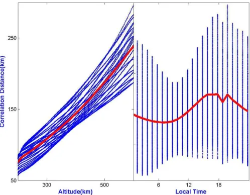
3.5 Vertical correlation distance

Altitude and local time variations of the vertical correlation distance are plotted in Fig. 5. When illustrating the altitude variations, all the results in the different local times are plot-ted together and the mean values are calculaplot-ted. The ver-tical correlation distance increases with an increase in alti-tude. The mean value varies from 75 km in 200 km altitude to 240 km in the 600 km altitude. According to the local time variations of the mean values in the different altitudes,

Figure 3a. Latitude variations of meridional correlation distance for the 12 selected local times. Sol

Fig. 3. (a) Latitude variations of meridional correlation distance for the 12 selected local times. Solid lines are the corresponding mean values of different seasons during 2000 and 2005.

obvious local time variations can be concluded. The verti-cal correlation distance is bigger in the daytime than in the night, which is consistent with that of the meridional corre-lation distance. The latitude and longitude variations of the vertical correlation distance cannot be investigated here, due to the choice of observations, and these will be studied in the future.

4 Discussion

4.1 The relative larger correlation between magnetic con-jugate points

Relative larger correlations of TEC’s day-to-day variabil-ities can be found between magnetic conjugate points from Fig. 2. Actually, the correlation between magnetic conjugate points has been found by several researchers. Yamamoto et al. (1995) observed electric fields fluctuations at magnetic conjugate points in both hemispheres simulta-neously. They suggested that these fluctuations are caused by field-aligned currents which flow from the ionosphere in one hemisphere to the conjugate point in the other hemi-sphere. Geomagnetic conjugate point airglow observations indicate that plasma depletions elongate along the geomag-netic field lines (Otsuka et al., 2002). According to Rishbeth and Mendillo (2001), these factors, including electric field fluctuations and field-aligned plasma flows, can result in the day-to-day variability of the ionosphere. Even medium-scale

traveling ionospheric disturbances (MSTID) at mid-latitude can also be observed at geomagnetic conjugate points si-multaneously (Otsuka et al., 2004). It can be interpreted by the polarization electric field which maps along the mag-netic field and moves the F region plasma upward or down-ward by E×B drifts, causing plasma density perturbations with structures mirrored in the Northern and Southern Hemi-spheres. Several sources of MSTID, such as atmospheric gravity waves that propagate upward from the lower atmo-sphere or are created in conjunction with auroral activity, au-roral joule heating, and other weather events, may also cause ionospheric day-to-day variability (Otsuka et al., 2004; Rish-beth and Mendillo, 2001). So the geomagnetic conjugacy of the above factors may also result in the corresponding ge-omagnetic conjugacy of the electron densities’ day-to-day variability. As indicated from Fig. 2b, the correlation coef-ficients between geomagnetic conjugate points have an obvi-ous decrease around sunrise and sunset at the upper latitude (60◦_{) and their values are bigger in the equinoxes than in} the solstices. These variations can simply be interpreted by the deviation of the magnetic meridian from the geographical meridian. Because of the existence of this deviation, some geographic regions in one hemisphere, where the dip lati-tudes are high, will have an earlier sunrise (sunset) than that from the magnetic conjugate-points in the other hemisphere. The time delay of sunrise (sunset) between the magnetic con-jugate points will result in the differences in the photoioniza-tion rates of the plasma. These differences are not notable at

X. Yue et al.: Statistical analysis on spatial correlation of ionosphere 1821

Figure 3b. Local time variations of meridional correlation distance in 12 selected latitudes for equino

Fig. 3. (b) Local time variations of meridional correlation distance in 12 selected latitudes for equinox (solid lines), summer (dash-dot lines), and winter (dashed lines), respectively.

low latitudes because of the little dip latitude there and are more obvious during solstice than during equinox because of the lack of uniform sunshine during the solstice between both hemispheres. One evidence of the above theory is the pre-sunrise ion temperature enhancement phenomena observed by ROCSAT-1 (Chao et al., 2003).

4.2 Variations of the correlation distance in three directions versus several factors

Many controlling factors, such as solar radiation, geomag-netic activity, and even seismic activity, may result in the ionospheric day-to-day variability (Rishbeth and Mendillo, 2001; Pulinets, 1998; Pulinets and Liu, 2004). Rishbeth and Mendillo (2001) have summarized almost all possible causes of the ionospheric F-layer variability and broadly di-vided them into four categories, which consist of solar ion-izing radiation, solar wind and geomagnetic activity, neutral atmosphere, and electrodynamics. Of these factors, solar ra-diation, geomagnetic activity, and meteorological sources are most frequently discussed. It is recognized that the mete-orological sources of the F-layer variability are comparable to the geomagnetic source and much larger than the solar component (Forbes et al., 2000; Fuller-Rowell et al., 2000; Mendillo et al., 2002; Rishbeth and Mendillo, 2001). Un-der geomagnetic quiet conditions, the variabilities of Nmaxat

high frequencies are mainly due to the meteorological influ-ences (Forbes et al., 2000). As can be imaged, the day-to-day

variabilities originating from different sources may have dif-ferent spatial correlation scales. This is mainly because some sources are global (e.g., solar radiation) while some are lo-calized (e.g., meteorological sources). Mendillo et al. (2002) found that the correlation scale size of meteorological distur-bances may be around 2500 km.

According to Forbes et al. (2000), ionospheric variabil-ity increases with magnetic activvariabil-ity at all latitudes and for both low and high frequency ranges, and the slopes of all curves increase with latitude. Thus, the responsiveness of the ionosphere to increased magnetic activity increases as one progresses from lower to higher latitudes. But they did not consider variations of in the variabilities versus lo-cal time and season. The local time and seasonal vari-ations the ionospheric F-layer variabilities are statistically obtained by Araujo-Pradere et al. (2005) and Rishbeth and Mendillo (2001) by analyzing global ionosondes observa-tions. A greater variability of NmF2 at night than by day and in winter than in summer was shown. Enhanced auroral energy input and the lack of the strong photochemical control of the F2-layer at night are considered to be the cause of this phenomenon (Rishbeth and Mendillo, 2001). These varia-tions of ionospheric variability indicate different dominating causes at different local times and latitudes, which may have different spatial correlation scales. These varied causes may result in the latitude and local time variations of the merid-ional correlation distance. The contrary latitude variations of

Figure 4. Local time variations of zonal correlation distance for the selected latitudes for equinox (so

Fig. 4. Local time variations of zonal correlation distance for the selected latitudes for equinox (solid lines), summer (dash-dot lines), and winter (dashed lines), respectively.

the meridional correlation distance around sunrise may have a relationship with the time delay of sunrise at the higher dip latitude, as well as the special electrodynamics factors at low latitudes. These factors include the sensitivity of anomaly peak densities to day-to-day variations in F-region winds and electric fields driven by the E-region wind dynamo (Forbes et al., 2000) or the equatorial electrojet strength (Dabas et al., 2006). Considering the seasonal variation of ionospheric variability, the lowest variability was typically found in sum-mer and the largest variability occurred in winter, with the equinox lying between the solstice extremes (Araujo-Pradere et al., 2005). From our results, the meridional correlation dis-tance also has obvious seasonal variations in mid-latitudes in the Northern Hemisphere. This may be originated from the differences in the meteorological disturbances between sum-mer and winter at mid-latitudes in the Northern Hemisphere (Yu et al., 2007). However, seasonal variations are not ev-ident in low latitudes or in the Southern Hemisphere. The influences of data coverage in Southern Hemisphere can also not be eliminated. For the zonal correlation distance, the lat-itude variations can partly be interpreted by the decrease in the zonal circle with the increase in latitude. In Southern Hemisphere, the zonal correlation distance is greater in the nightside than in the dayside in all seasons. Further statistical analysis and modeling are needed to investigate this problem. For the mid-latitude, with the increase in altitude, the effect

of the dynamical process becomes dominate. The effect of the dynamics process is more important at night than by day because of the absence of solar radiation at night. These vari-ations in the control factors probably result in the altitude and local time variations of the vertical correlation distance of the electron density. However, further investigations are needed to address this issue.

4.3 Influence of ionospheric storms on the spatial correla-tions

During the geomagnetic storms, the ionosphere presents prominent disturbances with the increased solar and mag-netospheric energy inputs, which is usually called an iono-spheric storm. Since it was first discovered, the ionoiono-spheric storm has been studied extensively by the researchers all over the world. Many excellent reviews on this topic have been published in the last few years (e.g. Buonsanto, 1999; Mendillo, 2006; Pr¨olss, 1995). In general, the patterns of ionospheric disturbances are different in different places (high, middle, and low latitude) and local times (day or night) during the same geomagnetic storm (Mendillo, 2006). It can generally be interpreted by the competitive results of differ-ent disturbed factors, including neutral wind, electric field, O/N2, and etc.

Many researchers have studied the local time, latitude, and seasonal variations of ionospheric negative and positive

X. Yue et al.: Statistical analysis on spatial correlation of ionosphere 1823

Figure 5. Altitude and Local time variations of vertical correlation distance. The solid lines in th

Fig. 5. Altitude and local time variations of the vertical correlation distance. The solid lines in the left panel are mean values of different local times and in the right panel are mean values of different altitudes.

storms by statistically analyzing the worldwide observations (Balan and Rao, 1990; Field and Rishbeth, 1997). In this pa-per, we did not consider the geomagnetic activity in the sta-tistical processes. So the derived correlations may probably be influenced by the occurrence of an ionospheric negative or positive storm.

As indicated from Fig. 2b, the correlations of conjugate points between equinox hemispheres (February–April and August–October) are greater than that between the summer and winter hemispheres (May–July and November–January). Aside that the asymmetry of solar energy input into the two hemispheres is more obvious in solstices than in the equinoxes, the different occurrence rates of ionospheric neg-ative or positive storms may also be an important cause. Ac-cording to Field and Rishbeth (1997) and Pr¨olss (1995), neg-ative storm effects are observed to extend all the way from the polar region to the subtropics during summer, while dur-ing winter they are restricted to the higher latitude region, and positive storms are mainly observed in winter. But these differences are not obvious in the equinox hemispheres. The different phases of the ionospheric storms which occurred in the winter and summer hemispheres may decrease the cor-relation coefficients between the conjugate points. In ad-dition, the difference in the motion directions of the mid-latitude/high-latitude trough may also decrease this correla-tion. It is shown from Fig. 3b, in the mid-latitude of the Northern Hemisphere (from 40◦_{to 60}◦_{), the meridional}

cor-relation distance is larger in summer than in the equinox and larger in equinox than in winter. As described above, it mainly occures during negative storms in summer in the mid-latitude (from 40◦_{to 60}◦_{), while in winter it is a transition} area between a negative and positive storm. It is also shown in Fig. 3b that the meridional correlation distance is larger in daytime than nighttime, except for the equatorial area. Ac-cording to Balan and Rao (1990) and Pr¨olss (1995), nega-tive storms at middle latitude are usually observed to follow magnetic activity which occurred during the preceding night, while positive ionospheric storms are generally associated with magnetic activity beginning in the local daytime sector. These local time variations of ionospheric negative/positive storms might contribute to the differences in the meridional distance between the daytime and night in the higher latitude.

5 Conclusions

In this paper, the spatial correlations of ionospheric day-to-day variability are investigated, for the first time, by statis-tical analysis on GPS and Incoherent Scatter Radar observa-tions in a global scale. The meridional correlaobserva-tions show sig-nificant (>0.8) correlations in the latitudinal blocks of about 6 degrees on average. Relative larger correlations of TEC’s day-to-day variabilities can be found between magnetic con-jugate points. This phenomenon may be due to the geo-magnetic conjugacy of several factors, such as electric field

fluctuations, field-aligned plasma flows, and the polarization electric field, which are the causes of the ionospheric day-to-day variability. The correlation coefficients between geo-magnetic conjugate points have an obvious decrease around sunrise and sunset at the upper latitude (60◦_{)and their values} are bigger between the winter and summer hemispheres than between spring and autumn hemispheres. The time delay of sunrise (sunset) between magnetic conjugate points with a high dip latitude is a probable reason. The asymmetry of the occurrence of a negative/positive storm in the solstices may also decrease the correlation.

In the daytime, the meridional correlation distance is big-ger in the mid-latitude than in the low and equatorial lati-tudes, while no evident latitude variations around midnight are found. However, around sunrise, the meridional correla-tion distance is larger in equatorial area than at mid-latitude. The meridional correlation distance is larger in day time than night time, but the arisen time of the maximum is different at different latitudes. The zonal correlation distance increases with the increase in latitude in both hemispheres. Except for in the mid-latitude of the Southern Hemisphere (between – 60◦_{and –40}◦_{), where the zonal correlation distance is larger} in the nightside than in the dayside, there is no distinct lo-cal time variation. The vertilo-cal correlation distance increases with the increase in altitude and is larger during the day than at night. These variations of the correlation distance of the ionospheric day-to-day variability versus different factors can generally be interpreted by the variations in the control-ling factors, which may have different spatial scales. The influences of the occurrence of ionospheric storms may not be ignored. Further modeling and data analysis are needed to address this problem.

As indicated by Araujo-Pradere et al. (2005), it may be more accurate when considering the variability of the ionosphere in ionospheric modeling and forecasting (Stanis-lawska et al., 1996). Specific representation of the spatial correlation of ionospheric day-to-day variability may also be valuable in ionospheric modeling, especially in practical use for space weather. Furthermore, our results are useful for constructing background covariance matrix when assimilat-ing observations into models, especially empirical models, by a 3DVAR or Kalman Filter method (Bust et al., 2004; Fuller-Rowell et al., 2006).

Acknowledgements. This work is supported by National Science

Foundation of China (40636032, 40574071) and National impor-tant Basic Research Project (2006CB806306). Millstone Hill data were obtained through the Madrigal Database which is assembled and maintained by members of MIT Haystack. The Global Iono-spheric Map data provided by the Jet Propulsion Laboratory are downloaded from the ftp site: ftp://cddis.gsfc.nasa.gov.

Topical Editor M. Pinnock thanks two anonymous referees for their help in evaluating this paper.

References

Araujo-Pradere, E. A., Fuller-Rowell, T. J., Codrescu, M. V., and Bilitza, D.: Characteristics of the ionospheric variability as a function of season, latitude, local time, and geomagnetic activity, Radio Sci., 40, RS5009, doi:10.1029/2004RS003179, 2005. Balan, N. and Rao, P. B.: Dependence of ionospheric response on

the local time of sudden commencement and the intensity of ge-omagnetic storms, J. Atmos. Terr. Phys., 52(4), 269–275, 1990. Bradley, P. A. and Cander, L. R.: Proposed terminology for the

clas-sification and parameters for the quantification of variability in ionosphere morphology, Annals of Geophysics, 45(1), 97–103, 2002.

Bradley, P. A., Kouris, S. S., Stanislawska, I., Fotiadis, D. N., and Juchnikowski, G.: Day-to-day variability of IRI electron density height profile, Adv. Space Res., 34, 1869–1877, 2004.

Buonsanto, M. J.: Ionospheric storms – A review, Space Sci. Rev., 88, 563–601, 1999.

Bust, G. S., Coker, C., Coco, D., Gaussiran II T. L., and Lauderdate, T.: IRI data ingestion and ionospheric tomography, Adv. Space Res., 27(1), 157–165, 2001.

Bust, G. S., Garner, T. W., and Gaussiran, T. L.: Ionospheric Data Assimilation Three-Dimensional (IDA3D): A global, multisen-sor, electron density specification algorithm, J. Geophys. Res., 109, A11312, doi:10.1029/2003JA010234, 2004.

Chao, C. K., Su, S.-Y., and Yeh, H. C.: Presunrise ion temperature enhancement observed at 600 km low- and mid-latitude ionosphere, Geophys. Res. Lett., 30, 1187, doi:10.1029/2002GL016268, 2003.

Dabas, R. S., Sharma, N., Pillai, M. G. K., and Gwal, A. K.: Day-to-day variability of equatorial and low latitude F-region ionosphere in the Indian zone, J. Atmos. Sol. Terr. Phys., 68, 1269–1277, 2006.

Field, P. R. and Rishbeth, H.: The response of the ionospheric F2-layer to geomagnetic activity: an analysis of worldwide data, J. Atmo. Sol. Terr. Phys., 59, 163–180, 1997.

Forbes, J. M., Palo, S. E., and Zhang, X. L.: Variability of the iono-sphere, J. Atmo. Sol. Terr. Phys., 62, 685–693, 2000.

Fox, M. W.: A simple, convenient formalism for electron density profiles, Radio Sci., 29(6), 1473–1491, 1994.

Fotiadis, D. N. and Kouris, S. S.: A functional dependence of foF2 variability on latitude, Adv. Space Res., 37, 1023–1028, 2006. Fuller-Rowell, T. J., Codrescu, M., and Wilkinson, P.: Quantitative

modeling of the ionospheric response to geomagnetic activity, Ann. Geophys., 18, 766–781, 2000.

Fuller-Rowell, T., Araujo-Pradere, E., Minter, C., Codrescu, M., Spencer, P., Robertson, D., and Jacobson, A. R.: US-TEC: A new data assimilation product from the Space En-vironment Center characterizing the ionospheric total electron content using real-time GPS data, Radio Sci., 41, RS6003, doi:10.1029/2005RS003393, 2006.

Gail, W. B., Prag, A. B., Coco, D. S., and Coker, C.: A statisti-cal characterization of lostatisti-cal mid-latitude total electron content, J. Geophys. Res., 98(A9), 15 717–15 728, 1993.

Huang, T. X.: Horizontal gradients and correlation coefficients in total electron content of the ionosphere, Chinese J. Geophys. (in Chinese), 26, 301–308, 1983.

Iijima, B. A., Harris, I. L., Ho, C. M., Lindqwister, U. J., Man-nucci, A. J., Pi, X., Reyes, M. J., Sparks, L. C., and Wilson, B. D.: Automated daily process for global ionospheric total electron

X. Yue et al.: Statistical analysis on spatial correlation of ionosphere 1825

content maps and satellite ocean altimeter ionospheric calibra-tion based on Global Posicalibra-tioning System data, J. Atmo. Sol. Terr. Phys., 61, 1205–1218, 1999.

Klobuchar, J. A., Doherty, P. M., and ElArini, M. B.: Potential ionospheric limitations to GPS Wide-Area Augmentation Sys-tem (WAAS), Navigation, 42(2), 1995.

Mannucci, A. J., Wilson, B. D., Yuan, D. N., Ho, C. H., Lindqwis-ter, U. J., and Runge, T. F.: A global mapping technique for GPS-derived ionospheric total electron content measurements, Radio Sci., 33(3), 565–582, 1998.

Mendillo, M., Rishbetha, H., Roble. R. G., and Wroten, J.: Mod-elling F2-layer seasonal trends and day-to-day variability driven by coupling with the lower atmosphere, J. Atmos. Sol. Terr. Phys., 64, 1911–1931, 2002.

Mendillo, M.: Storms in the ionosphere: Patterns and pro-cesses for total electron content, Rev. Geophys., 44, RG4001, doi:10.1029/2005RG000193, 2006.

Miro Amarante, G., Cuteo Santamaria, M., Mosert de Gonzalez, M., Radicella, S. M., and Ezquer, R.: Day-to-day changes in experimental electron density profiles and their implications to IRI model, Adv. Space Res., 34, 1878–1886, 2004.

Nisbet, J. S., Tyrnov, O. F., Zintchenko, G. N., and Ross, W. J.: Limits on the Accuracy of Correction of Trans-ionospheric Prop-agation Errors by Using Ionospheric Models Based on Solar and Magnetic Indices and Local Measurements, Radio Sci., 16, 127– 133, 1981.

Otsuka, Y., Shiokawa, K., Ogawa, T., and Wilkinson, P.: Geomag-netic conjugate observations of equatorial airglow depletions, Geophys. Res. Lett., 29, 1753, doi:10.1029/2002GL015347, 2002.

Otsuka, Y., Shiokawa, K., Ogawa, T., and Wilkinson, P.: Geomagnetic conjugate observations of medium-scale trav-eling ionospheric disturbances at midlatitude using all-sky airglow imagers, Geophys. Res. Lett., 31, L15803, doi:10.1029/2004GL020262, 2004.

Pr¨olss, G. W.: Ionospheric F-Region Storms, in: Handbook of At-mospheric Electrodynamics, vol.2, edited by: H. Volland, chap. 8, pp. 195–248, CRC Press, Boca Raton, Fla., 1995.

Pulinets, S. A.: Seismic activity as a source of the ionospheric vari-ability, Adv. Space Res., 22, 903–906, 1998.

Pulinets, S. A. and Liu, J. Y.: Ionospheric variability unrelated to solar and geomagnetic activity, Adv. Space Res., 34, 1926–1933, 2004.

Richmond, A. D.: Ionospheric electrodynamics using magnetic apex coordinates, J. Geomagn. Geoelectr., 47(2), 191–212, 1995. Rishbeth, H.: How the thermospheric composition affects the iono-spheric F2-layer,J. Atmos. Sol. Terr. Phys., 60, 1385–1402, 1998. Rishbeth, H. and Mendillo, M.: Patterns of F2-layer variability, J.

Atmo. Sol. Terr. Phys., 63, 1661–1680, 2001.

Rush, C. M.: An ionospheric observation network for use in short-term propagation predictions, Telecommun. J., 43(8), 544–549, 1976.

Saito, A., Iycmori, T., Sugiura, M., Maynard, N. C., Aggson, T. L., Brace, L. H., Takeda, M., and Soicher, H.: Spatial Correlation of Transionospheric Signal Time Delays, IEEE Transactions on Antennas and Propagation AP-26, 3, 1978.

Stanislawska, I., Juchnikowski, G., and Cander, Lj. R.: Kriging method for instantaneous mapping at low and equatorial lati-tudes, Adv. Space Res., 18(6), 217–220, 1996.

Yamamoto, M.: Conjugate occurrence of the electric field fluctua-tions in the nighttime midlatitude ionosphere, J. Geophys. Res., 100(A11), 21 439–21 451, 1995.

Yu, X., Wan, W., Liu, L., Yue, X., and Xu, G.: Correlation distance of NmF2’s day-to-day variability in Europe, Chinese J. Geophys., (in Chinese), 50(5), 1283–1288, 2007.