Design of Annular Fuel for High Power
Density BWRs
831 V&
1-by l HV4
Paolo Morra AE)O1ONlHO- O
Laurea in Ingegneria Nucleare |3ULLSNI SLL3SflHOss
La Sapienza University, 2003
Submitted to the Department of Nuclear Engineering ARCHIVES
in partial fulfillment of the Requirements for the Degree of
MASTER of SCIENCE in Nuclear Engineering
at the
MASSACHUSETTS INSTITUTE OF TECHNOLOGY
0sevq 200 z5December 2004
© 2004 Massachusetts Institute of Technology, all rights reserved
Author
-A
uthor.
...
....
o
....
.. ...
...
..
-..
...
Paolo Morra, MITDepartment of Nuclear Engineering December 2004 Certified by ...
Q A jid S. Kazimi, MIT Professor of Nuclear Engineering Thesis Supervisor Certified by ... ...
Pavel Hejzlar, MIT Principal Research Scientist
'~k ? v X Thesis Reader
Accepted
by... . .. ...
Jeffrey Coderre Professor of Nuclear Engineering
Design of Annular Fuel for High Power
Density BWRs
by
Paolo Morra
Submitted to the Department of Nuclear Engineering on December 17, 2004, in partial fulfillment of the Requirements for the Degree of Master of Science at the
Massachusetts Institute of Technology
ABSTRACT
Enabling high power density in the core of Boiling Water Reactors (BWRs) is economically profitable for existing or new reactors. In this work, we examine the potential for increasing the power density in BWR plants by switching from the current solid fuel to annular fuel cooled both on its inside and outside surfaces. The GE 8x8 bundle dimensions and fuel to moderator ratio are preserved as a reference to enable applications in existing reactors. A methodology is developed and VIPRE code calculations are performed to select the best annular fuel bundle design on the basis of its Critical Power Ratio (CPR) performance. Within the limits applied to the reference solid fuel, the CPR margin in the 5x5 and 6x6 annular fuel bundles is traded for an increase in power density. It is found that the power density increase with annular fuel in BWRs may be limited to 23%. This is smaller than possible for PWRs due to the different mechanisms that control the critical thermal conditions of the two reactors. The annular fuel could still be a profitable alternative to the solid fuel due to neutronic and thermal advantages.
Acknowledgements
I would like to express my gratitude to the Nuclear Engineering Department at MIT for giving me the opportunity to pursue my study as a graduate student in such an awesome environment. MIT is not only my dream school from an academic point of view but helped me also to develop personal qualities like tenacity, diligence and ability to work in teams.
I would like to thank in particular my advisor, Professor Mujid S. Kazimi for his pedagogical, financial and personal support during my stay at MIT. Special thanks go to Dr. Pavel Hejzlar and Dr. Pradip Saha for their help in my research and my personal formation. Their help has been invaluable.
I also thank Christopher S. Handwerk, Dandong Feng and Zhiwen Xu for the useful discussions.
I would like also to thank to my family and my friends for their unwavering support. A special thanks in particular to the ones that shared with me the endless nights in the office.
But in particular I would like to dedicate this work to my grandfather Roccantonio Morra. I will never forget you.
Table of Contents
Abstract ... 3
List of Figures...7
List of Tables ... 9
Chapter 1: Introduction and Scope of the Work ... 10
Chapter 2: Methodology and Analysis Tools ... 13
2.1 MNethodology...13
2.2 Analysis tools ... 19
2.3 VIPRE thermal hydraulic model and correlation choices ... 22
2.3.1 The flow model ... 23
2.3.2 Heat transfer correlations ... 24
2.4 CPR correlations ... 25
2.5 CPR correlation modifications ... 28
Chapter 3: Fuel Modeling ... 31
3.1 Solid fuel bundle geometry ... 31
3.1.1 Geometrical data ... 31
3.1.2 Other data ... 35
3.2 Annlmular fuel design ... 39
3.2.1 Criteria for the bundle design ... 39
3.2.2 Geometrical data ... 45
3.2.2.1 The 5x5 bundle ... 45
3.2.2.2 The 6x6 bundle ... 48
3.2.3 Other data ... 51
3.3 Differences between the 5x5 and the 6x6 design ... 54
Chanter 4: Results ... 56
4.1.4 MCPR ... 63
4.2 Data presentation ... 69
4.2.1 Annular 5x5 ... 69
4.2.1.1 Thermal hydraulic parameters ... 69
4.2.1.2 MCPR ... 74
4.2.2 Annular 6x6 ... 76
4.2.2.1 Thermal hydraulic parameters ... 76
4.2.2.2 MCPR ... 85
4.3 Analysis of the results ... 87
4.3.1 Theoretical expectations on CPR ... 88 Chapter 5: Conclusions ... 91 5.1 Summary ... 91 5.2 Conclusions ... 92 5.3 Future studies ... 93 References ... 94
Appendix A: Convergence and Comparison Criteria ... 95
A.1 Convergence ... 95
A.2 Comparison criteria ... 99
Appendix B: Vipre inputs ... 102
B.1 Solid fuel-average bundle input ... 102
B.2 Solid fuel-hot bundle input ... 108
B.3 Annular 5x5-average bundle input ... 114
B.4 Annular 5x5-hot bundle input ... 120
B.5 Annular 6x6-average bundle input ... 126
B.6 Annular 6x6-hot bundle input ... 133
Appendix C: MatLab Inputs for Annular Fuel Design ... 141
Appendix D: MatLab Inputs for Solid Fuel Design ... 148
D. 1 Annular 5x5 ... 148
D.2 Annular 6x6 ... 165
List of Figures
Figure 2.1: Flow chart of the fuel comparison ... 15
Figure 2.2: Flow chart of the iterative method for the thermal hydraulic calculations .... 18
Figure 2.3: Flow chart of the code interactions ... 21
Figure 3.1: 2D view of a typical BWR-5 8x8 bundle ... 34
Figure 3.2: Solid fuel axial power peaking ... 36
Figure 3.3: BWR-5 8x8 radial power peaking ... 37
Figure 3.4: Solid fuel rod section ... 41
Figure 3.5: Annular fuel rod section ... 41
Figure 3.6: Solid fuel rods layout in respect to the bundle wall ... 42
Figure 3.7: Annular fuel rods layout in respect to the bundle wall ... 43
Figure 3.8: 21) view of the annular fuel 5x5 bundle ... 47
Figure 3.9: 2D view of the annular fuel 6x6 bundle ... 50
Figure 3.10: Radial power peaking for the 5x5 annular fuel bundle ... 51
Figure 3.11: Radial power peaking for the 6x6 annular fuel bundle ... 52
Figure 4.1: Void fraction and quality in a typical BWR [9] ... 57
Figure 4.2: Vo)id fraction in the solid fuel model ... 58
Figure 4.3: Equilibrium quality in the solid fuel model ... 59
Figure 4.4: Quality in the hot channel of the solid fuel model ... 60
Figure 4.8: MCPR in the solid fuel model ... 65
Figure 4.9: MCPR comparison with reference (10% error bar) ... 66
Figure 4.10: MCPR comparison with reference (5% error bar) ... 67
Figure 4.11: Hot channel quality axial profile for annular 5x5 design at 100% power .... 71
Figure 4.12: Hot channel quality axial profile for annular 5x5 design at 116% power .... 72
Figure 4.13: Pressure drop increase with power for annular fuel 5x5 ... 73
Figure 4.14: MCPR for the annular fuel 5x5 ... 74
Figure 4.15: Power increase for annular fuel 5x5 ... 75
Figure 4.16: Hot rod temperature comparison ... 78
Figure 4.17: Part of the 6x6 bundle layout ... 79
Figure 4.18: Hot rod channel quality axial profile for annular 6x6 design at 100% power ... 80
Figure 4.19: Hot rod channel quality axial profile for annular 6x6 design at 123% power ... 81
Figure 4.20: Hot channel (corner) quality axial profile for annular 6x6 design at 100% power ... 82
Figure 4.21: Hot channel (corner) quality axial profile for annular 6x6 design at 123% power ... 83
Figure 4.22: Pressure drop increase with power for annular fuel 6x6 ... 84
Figure 4.23: MCPR for the annular fuel 6x6 ... 85
List of Tables
Table 3.1: Design parameters of the GE BWR 8x8 bundle ... 32
Table 3.2: Core conditions of the GE BWR 8x8 bundle ... 33
Table 3.3: Local pressure drop coefficients ... 38
Table 3.4: Armular fuel 5x5 possible designs ... 45
Table 3.5: Geometrical parameters of the Annular fuel 5x5 possible designs ... 46
Table 3.6: Annular fuel 6x6 possible designs ... 48
Table 3.7: Geometrical parameters of the Annular fuel 6x6 possible designs ... 49
Table 3.8: Comparison between the 5x5 and the 6x6 annular designs ... 54
Table 4.1: Thermal hydraulic comparison for the 5x5 annular fuel design ... 70
Table 4.2: Thermal hydraulic comparison for the worse conditions (5x5 annular fuel) ... 70
Table 4.3: Thermal hydraulic comparison for the 6x6 annular fuel design ... 76
Table 4.4: Thermal hydraulic comparison for the worse conditions (6x6 annular fuel) ... 77
Table 4.5: Fuel design comparison ... 88
Chapter 1
Introduction and Scope of Work
There is a close correlation between the energy consumed per capita and the quality of life in any society. One of the biggest challenges of modem times is to provide a longer and better life to the increasing world population; the energy needed for such a goal cannot be sustained in the long term simply by increasing energy efficiency nor can it be reasonably achieved using the current fuel mix. The increasing tension in the oil-rich Middle East and the depletion of fossil fuel resources in the rest of the world foretell a future where energy is going to be more and more expensive. Thus the average quality of life of the world population may suffer if there is no change or innovation in energy technology and policy.
Currently, worldwide research is exploring many directions to find a solution for sustainable energy, and most of the probable alternatives involve a larger role for nuclear power in modem societies. This will be hard to achieve through building of new nuclear power units due to the resistance of a significant segment of the population to nuclear energy. Eventually the situation may change, but as a short to medium term solution, the global nuclear industries are pursuing relicensing and power uprating of already existing nuclear power plants. Due to the high capital cost of nuclear plants, either extending the life of a plant or raising its power output would be economic, since most of the added energy is obtained with a smaller investment, if any, in capital costs.
Power uprating of existing Nuclear Power Plants (NPPs) has been thoroughly studied and extensively applied by improving the methods to evaluate the conservative margin between the operating and limiting condition, or by increasing the capability of the secondary coolant circuit. One way to raise the power in a major way is to change the fuel design in the reactor core. If the more efficient fuel design can be accommodated in
the existing plants, upgrading can be considered. Alternatively, the increased power density of the core can be the basis for new power plants.
A new fuel design for Pressurized Water Reactors (PWR) has been proposed and studied at MIT. The fuel employs annular geometry with internal as well as external cooling, to be able to lower the cladding heat flux and thus achieve higher safety margins than the normal solid fuel. These larger margins allow raising the power of the plant without compromising its safety in case of accidents. The PWR annular fuel study shows promising results [1]. It is reasonable to expect a substantial power density increase to have a significant impact on the revenues of the nuclear industry even considering the higher manufacturing costs of the annular fuel.
The very promising results obtained for the PWR annular fuel naturally led to the proposal to investigate the possibility of a power density upgrade in the Boiling Water Reactor (BWR) plants using the same technique. There is no other study that we are aware of examining the annular fuel for BWR application. So the scope of this work is to provide a first estimate of the possibility of using the annular fuel in BWR plants and to find what the most promising designs are. To identify the power uprate potential, it is necessary to quantify safety margins of the core with annular fuel. The Critical Power Ratio (CPR) is used to quantify the safety margin during steady state operation and transients, as is current practice for the solid fuel in BWR plants.
First, we will examine the possible designs of the BWR bundle with the goal of maximizing the advantage given by the annular fuel (in particular the heat transfer area). Two layouts will be studied in particular, a 5x5 and a 6x6 fuel bundle, but under the constraint of fixed bundle size equal to the GE 8x8 solid fuel bundle. The constraints on the design, especially the minimum gap between rods, the same assembly size as existing BWRs, and a minimum allowable diameter of the internal channel, combine to limit
The methodology and analysis tool are described in Chapter 2. The possible correlations for CPR calculation, will be adapted to annular fuel, and implemented in the VIPREOlmodO2 code (Chapter 2). Then on the basis of their thermal hydraulic characteristics (especially the heat transfer surface and the tightness of the pitch) we will select the most promising designs for a more in-depth study (Chapter 3). In this work, the coolant flow in the core is assumed to increase in proportion to the power density increase. We will also compare the annular fuel design to the solid fuel design and calculate the maximum power density upgrade achievable keeping the same safety margin as the solid fuel (Chapter 4). Finally, the work will be summarized and suggestions are made for future work (Chapter 5). Details of the code handling are given in the Appendices.
Chapter 2
Methodology and Analysis Tools
2.1 Methodology
Our objective, as stated in Chapter 1, is to show that switching to annular fuel in existing BWR cores can allow us to eventually raise the power with relatively small modifications to the plant, or at least to show that this possibility is interesting enough to be worth studying more in depth.
First we will consider that the limiting factor in the fuel assembly design is the CHF (Critical Heat Flux), and in particular, in the BWR case, the CPR (Critical Power Ratio) [2]. Thus we will evaluate the performance of the fuel designs on the basis of their CPR values, considering a fuel design better than another if its CPR is higher. By 'better' we mean that a fuel design with higher CPR than another will allow us to get a larger power increase. To maintain the same thermal environment under which the materials operate in the core as well as in the hot region of the vessel, we assume that the core flow will increase proportionally with the power, so that the steam flow rates (or quality) and pressure conditions of the hot assembly and the upper core regions are not altered. Also, for safety reasons, we will not allow the CPR of the annular fuel to be lower than the solid fuel value, following the reasoning that experience has shown the solid fuel to be reliable and safe and thus the annular fuel should be at least as good as the solid (at least in steady state) if it respects the same CPR constraint. This is further discussed in Section 2.4.
a BWR using normal (solid) fuel. After calculating the thermal hydraulic parameters, we can use them and a CPR (Critical Power Ratio) correlation to obtain the Minimum Critical Power Ratio (MCPR) of the two systems. We can also iterate on the possible designs of annular fuel to get the maximum possible power while keeping the MCPR equal or higher than that of the solid fuel.
If the MCPR of the annular fuel is larger than the solid fuel we can raise the power (and the mass flow rate by the same ratio) of the annular fuel till we reach the same MCPR of the solid fuel. This will give us an idea of how much we can improve the power in existing BWRs by switching to annular fuel. As expected, we will see in Chapter 4 that there exist annular fuel designs that have larger MCPR than the solid's, so we can obtain
Annular fu( benefic BWF el is not I TC'_ al or Ls Choose an annular fuel design and
calculate its MCPR Calculate the MCPR of the solid fuel reference Choose another annular fuel design
Compare the two and keep the one with larger MCPR
l
Calculate its MCPR
Compare the annular fuel and
the solid fuel MCPR NO
annular\
MCPR/ 'arger/ YFSRaise the power till the two have the same MCPR I, I -<1 _..-I /
-Now we would like to discuss in-depth the various parts of our methodology. First of all we note that while the whole process is once-through, it involves at least two large iteration loops, one to choose the best annular fuel design and the second to determine how much we can increase the power till we get the same MCPR as the solid fuel case. We will discuss in Section 2.3 why and how we are using the CPR as the main parameter in our analysis.
The iteration to choose the best annular fuel design is explained in-depth in Chapter 3. The possible designs are infinite, due to the fact that the geometrical variables in play are continuous. However with an intelligent choice of the parameters to explore and considering the many constraints we have to impose to get a fuel design that is viable from the mechanical, vibration, thermal hydraulic and neutronic points of view, we can limit our search to a few main designs. Also, we want to enable the fuel use by existing BWR plants and this forces more constraints on us.
The choice of the solid fuel reference arrangement and operating conditions is also shown in Chapter 3. In Chapter 4 we show the MCPR calculation for annular and solid fuel and the fact that annular fuel design that has higher MCPR than the solid can also satisfy the applied constraints. The power upgrade calculation is also shown in Chapter 4.
There is an additional feature that we wish to discuss here. In general to have an accurate thermal analysis the entire core should be modeled to have a complete thermal hydraulic
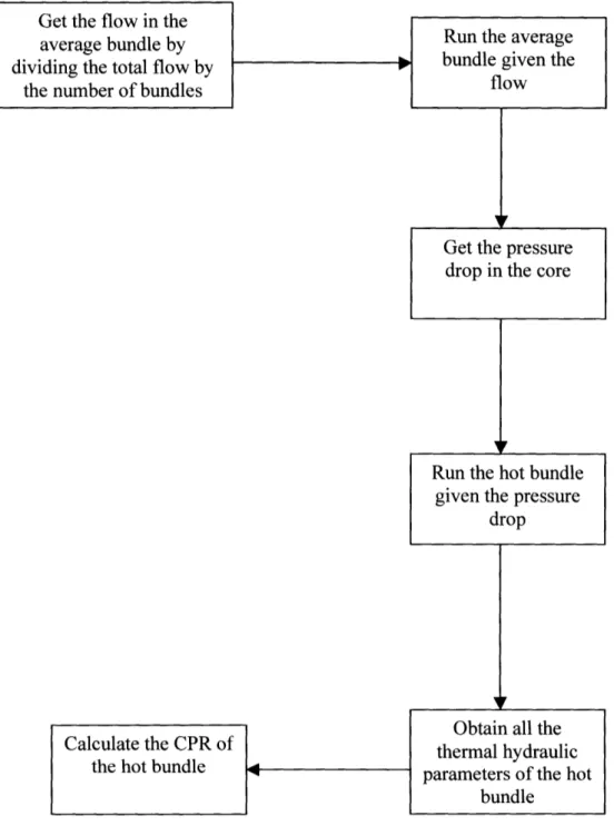
picture of the flow and consider the MCPR calculations reliable. In the BWR case though, we can resort to model only a bundle due to the fact that bundles are encased and share the same inlet and outlet plena. As a consequence we can consider the pressure drop the same for all bundles. This observation and the fact that there is no cross flow among the bundles allow us to calculate the MCPR of the BWR core using just two bundle models in the following way.
First we divide the total reactor flow, a commonly known data [2], by the number of bundles in the core (after considering that some of the flow will bypass the bundles) thus
getting the flow in an average bundle. Then, we use the model to calculate the pressure drop in the average bundle that, by the argument discussed before is going to be the same in every bundle. So, knowing the pressure drop we can apply the calculated pressure drop to the hot bundle model, this time to calculate the flow and all the other thermal hydraulic parameters. With these we can calculate the CPR of the hot bundle that will be the MCPR of the core. We use this method for both the annular and solid fuel and obtain the power density to match the MCPR of the two.
We want to underline that we developed two inputs for every design, one for the hot bundle and one for the average bundle. They have the same geometry and differ only in the power, the inlet pressure drop and the fact that they are used for different purposes in our method.
Calculate the CPR of
the hot bundle *
Run the average bundle given the
flow
!~~
Get the pressure drop in the core
Run the hot bundle given the pressure
drop
Figure 2.2: Flow chart of the iterative method for the thermal hydraulic calculations
Get the flow in the average bundle by dividing the total flow by
the number of bundles
Obtain all the thermal hydraulic parameters of the hot
2.2 Analysis Tools
As discussed in Section 2.1 it is important to choose a reliable thermal hydraulic code to do the calculations we have described. We need a code that has the following characteristics:
* has a robust thermal hydraulic model * widely accepted in the nuclear field
* able to calculate the thermal hydraulic parameters we need * allow change of the geometry of the fuel from solid to annular * numerically stable
* should have the possibility to calculate the CPR of the system * should have updated CPR correlations
* must be available to us * should be fast
* extensively documented
We have found that among the alternatives available to us, the VIPRE code fulfills better these characteristic. We had the VIPREOl1modO2 available and we decided to use it for this analysis since it meets all the above requirements and there was already some experience in its use in our department.
We have obtained good results with VIPRE, even if we had some problems with its convergence, especially in the annular fuel case. The code shows a tendency of not converging for a high number of axial nodes and there are peculiar zones where we cannot achieve convergence even with a lower number of axial nodes. It seems that the code has some problems in handling our model from the numerical point of view, because the principal cause of no convergence is due to the fact that the error keeps
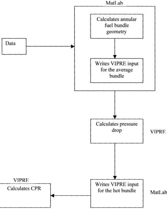
To implement the model explained in Section 2.1 we have scripted in MatLab a program (Appendices C and D) that calculates the fuel geometry and writes automatically the input for VIPRE (Appendix B). The MatLab script is able to write the input for both the average and hot bundles, thus we need to iterate between MatLab and VIPRE to get the MCPR of the design, as shown in Figure 2.3 below.
PI.
Calculates pressure drop
VIPRE
Calculates CPR I
Figure 2.3: Flow chart of the code interactions
Matlab
Data
Calculates annular fuel bundle
geometry
Writes VIPRE input for the average
bundle
Fr
VIPRE
Writes VIPRE input
for the hot bundle MatLab
2.3 VIPRE thermal hydraulic model and correlation
choices
VIPRE thermal hydraulic two phase flow model is essentially a homogeneous equilibrium model with an added set of void-drift correlations that help it better simulate the two phase effects. In fact the basic equations are written using the homogeneous formulation, and then the empirical correlations are added to refine the result.
The main assumptions are [3]:
* The flow has sufficiently low velocity such that kinetic and potential energies are small compared to internal thermal energy
* Work done by body forces and shear stresses in the energy equation is small compared to surface heat transfer and convective energy transport
* Heat conduction through the fluid surface is small compared to convective energy transport and heat transfer from solid surfaces
* The phases are in thermal equilibrium (except for subcooled boiling, see Section 2.3.1)
* Gravity is the only significant body force in the momentum equation
* Viscous shear stresses between fluid elements are small compared to the drag force on solid surfaces
* The fluid is incompressible (with respect to pressure) but thermally expandable; this means that the density and transport properties vary only with the local temperature, not with the pressure.
The above assumptions allow the conservation equations to be written in a simpler form but to get closer to reality the developers of the code inserted some correlations that allow them to close the mathematical system and to model more complicate situations with good accuracy.
2.3.1 The flow model
VIPRE 01 originally used the homogeneous model for two phase flow. This means that it considered the two phase flow to be a single fluid with the properties (density, viscosity, etc.) of the mixture, and the same phasic velocity for both the liquid and the vapor. This is a fairly reasonable approximation of the flow field at high pressures and high mass velocities, but is less satisfactory at lower pressures and mass velocities. The homogeneous model was modified in VIPRE01 mod 2.0 by the following correlations:
* Two phase friction multiplier
The momentum equation can be modified by this correlation that takes into account the nonhomogeneities in the two phase flow field and its influence on the pressure drop.
Here we use the EPRI correlation as suggested in the manual
* Subcooled void correlation
This correlation is used to model the nonequilibrium transition from single phase liquid to two-phase boiling flow with heat transfer from a hot wall. The correlation calculates the actual flowing quality for the two-phase mixture and the bulk liquid temperature which could still be subcooled.
Again we choose the EPRI correlation as suggested in the manual
* Bulk void relation
This correlation takes the local quality from the previous correlation and uses it to predict the subcooled void.
combination of the three EPRI correlations was shown to achieve the best results over the full range of void fractions [4].
2.3.2 Heat transfer correlations
The code uses the following correlations to calculate the heat transfer coefficient between the hot wall and the fluid. We must specify a correlation for each part of the boiling curve.
* Single phase forced convection
Here we choose the Dittus-Boelter correlation due to the fact that it covers our range of applications and requires one parameter less than the default correlation
(EPRI)
* Subcooled nucleate boiling
Here the only two available correlations that are valid for annulus are the Thom and Chen correlations. The Chen correlation was selected due to its wider applicability range. In any case both were tested and gave very similar results.
* Saturated nucleate boiling
Again the Chen correlation was selected for the same reasons as above
* Critical heat flux correlation
This correlation is used to define the peak of the boiling curve. The default (EPRI) correlation was selected. The correlation used for determination of CPR is different and will be discussed in the following Section.
* Transition boiling correlation
Film boiling correlation
We use the default correlation (Groeneveld 5.7)
All the correlations selected were checked to be applicable to our case or at least to be the closest to our conditions. Special attention has been given in selecting the correlations to be valid for annular geometry whenever possible.
2.4 CPR correlations
The phenomenon variously known as critical heat flux, departure from nucleate boiling, dryout or burnout is defined by Hewitt [5] as the condition where, for a relatively small increase in the heat flux, the heat transfer surface exhibits an inordinate increase in temperature.
However one chooses to define it, the critical heat flux (CHF) represents the sharp pinnacle of the boiling curve (by that we mean the curve that plots heat flux versus wall temperature), to the left of which is efficient stable nucleate boiling heat transfer and to the right of which is an inefficient unstable transition boiling region followed by film boiling leading to high surface temperatures. The point where this occurs in a particular two phase flow situation appears to depend on at least four distinct and nominally independent parameters: the geometry of the flow channel (usually taken into account through the hydraulic diameter), the pressure, the mass flow rate, and the quality (usually the equilibrium quality). These four parameters can be correlated from CHF test data to develop an equation defining the critical heat flux.
nucleate boiling (DNB). This phenomenon is most common in Pressurized Water Reactors (PWRs). In the higher steam quality region, mostly annular flow, the boiling crisis originates from depletion of the liquid film (film dryout). This is most common in Boiling Water Reactors (BWRs), and is the phenomenon we will concentrate upon.
In annular flow there is a thin liquid film in contact with the heated surface and in the middle of the channel there is vapor, usually with some liquid drops suspended in it, if the quality is not already very high. The flow rate of the liquid film is determined by evaporation, droplet entrainment (due to drops of liquid being suspended in the vapor that flows faster than the film thus creating film surface oscillation that allow some of the crests to become captured in the vapor) and droplet deposition back on the film. The first phenomenon is due to the heat flux coming from the solid surface, while the other two are originated by the mass exchange between the two phases due to the mechanical effect of the vapor on the liquid film.
After this description it is easy to see that the CHF corresponds to the condition in which the flow rate of the liquid film falls to zero. In this situation the solid wall 'dries out' of liquid and is forced to exchange heat directly with the vapor. Even if there will be liquid droplets suspended in it (because the quality is still less than 1), the heat transfer coefficient will diminish considerably compared to the boiling situation when the liquid film was still in contact with the wall. As a consequence, since the heat flux is constant during this process, the temperature difference will rise and the situation can become dangerous for the wall materials due to loss of strength at high temperatures or even approaching the melting point.
In DNB analysis for PWRs, the characteristic parameters are the critical heat flux (CHF), and the minimum departure from nucleate boiling ratio (MDNBR), which is equal to the minimum heat flux ratio (MCHFR).
Basically a correlation gives us the critical heat flux for the local thermal hydraulic
\/. 1I \/ 1
parameters and we also know the local heat flux , thus we can get the
minimum value of the ratio of the two:
1 11 I
(2.1)
This approach was originally used for BWRs as well. Today though in the most widely used approach for analysis of the boiling transition in BWRs, the characteristic parameters are the critical quality, the critical power and the critical power ratio (CPR).
VIPRE offers two correlations to calculate the thermal margin in a BWR, namely, the Hench-Levy correlation [3] and the Hench-Gillis correlation [3, 6]. The Hench-Levy correlation uses the older, less precise approach of calculating the MCHFR (the only difference being that it uses bundle average conditions to calculate the critical heat flux). Thus the Hench-Gillis correlation was selected since it uses the more modern CPR approach.
The Hench-Gillis correlation is used in iteration on bundle enthalpy rise to determine the critical bundle power. The bundle-average flow and enthalpy are used to calculate a critical quality value at every axial elevation along the boiling length. The critical
quality is compared then to the local bundle average quality to define the minimum
thermal margin (TM).
~~~~~~/ ~(2.2)
where
= factor function of the radial peaking Pressure
= critical quality calculated with the correlation at the boiling length corresponding to the axial location z
\!
= bundle average quality at axial location z = inlet subcooling for the bundle
= latent heat of vaporization at the system pressure
When the critical quality is equal to the local quality the equation is an exact balance and we have TM=1. In general the conditions will not be at critical power though, so the code will have to iterate on the average enthalpy till it strikes the right balance. The iteration will stop when TM=1 and then the enthalpy calculated will be used to compute the critical power. Then we can define:
k .,/.
It should be noted that the iterations are carried out only on the enthalpy rise of the bundle; the flow solution is not recomputed for the new power. This is consistent with the derivation of most critical quality correlations [3].
2.5 CPR correlation modification
The Hench Gillis correlation has the form [6]:
\!
(2.4) where the J-factor is principally a function of the radial power peaking. A and B are empirical functions of the mass flux (G), and:
1J) r\
where (D) is the diameter of the rods and (n) the number of rods.
. . . .
This 'Z' is the definition of the nondimensional boiling length that Hench and Gillis chose for their study. Since most of the parameters in the correlation are bundle-averaged, and thus similar if not identical both in the annular and solid fuel, it is evident that any advantage of the annular fuel will come from the 'heat transfer area' term in the
nondimensional boiling length.
Although VIPRE allows us to define tubes in the core and we use this option to simulate annular fuel, the CPR correlation uses only the external diameter to calculate the heat transfer area. This way in many cases we would have an even lower heat transfer area in the annular fuel case, thus eliminating any advantage that the annular fuel could present. Our solution was to include the internal diameter in the nondimensional boiling length calculation so that it would look as:
(2.6)
where is the external diameter of the annular fuel and the internal. While logical, this modification needs experimental verification.
We then created a new routine for CPR calculation in the VIPRE source code that is identical to the old routine besides the calculation of the heat transfer area. Using Equation 2.6 to calculate the nondimensional boiling length, we have the advantage of being able to consider all the heat transfer area in the annular fuel case, while the equation works as before for the solid fuel.
We consider our change of the correlation in line with the original idea of its development, since we have followed its theoretical aim: to consider the whole heat transfer area in Equation 2.5.
modem BWRs. It is important to note that it is a purely empirical correlation and thus should not be applied to conditions outside the range of validation data. We are perfectly aware that our change of the correlation for the annular fuel has no rigorous basis without extensive experimental testing. We are confident though that for our aim of giving an idea of the possible advantages of the annular fuel over the solid fuel it can help us form an informed opinion about the desirability of studying more in depth the use of annular fuel for BWRs
Chapter 3: Fuel Modeling
3.1 Solid fuel bundle geometry
In this work we propose to model both the solid and annular fuel bundles and compare the results. We are aware that the numbers we obtain are associated with uncertainties that we cannot firmly establish, but we are confident that the comparison to the solid fuel bundle can give us an indication on how good the annular fuel could be as an alternative.
The model we have used did not describe the conditions of a particular plant. We have tried to be as close as possible to the characteristics given in the open literature about the BWR plants now in operation (BWR-5) but we acknowledge the fact that no particular plant was the basis for it.
3.1.1 Geometrical data
We have chosen to test our designs using the flow conditions of the GE BWR5 plant, with the warning given above about the fact that we didn't have access to the characteristics of any particular plant. For this reason the BWR5 bundle was modeled generically using the VIPRE thermal hydraulic code, and we used that as a reference. The data we used as a reference for the GE BWR5 8x8 bundle are:
Table 3.1: Design parameters of the GE BWR 8x8 bundle
Parameters Values
Core thermal power (MWth) 3293
Number of fuel assemblies in the core 764
Active fuel height (cm) 367
Fuel assembly pitch (cm) 15.24
Bundle lattice 8x8
Lattice pin pitch (cm) 1.62
Clad thickness (cm) 0.085
Gap thickness (cm) 0.01
Number of fuel rods 62
Number of water rods 2
Inner distance between box walls (cm) 13.4
Fuel rod OD (cm) 1.23
Water rod OD (cm) 1.50
Water rod ID (cm) 1.32
Most of the geometrical data we have used can be extrapolated from the data of Table 3.1. These data are mostly from the BWR whole core sample input given in the VIPRE manual [7]. However that input is explicitly declared as a mix of BWR5 and BWR6 data, and was not referenced for a particular plant. This should not affect our work which does not aim to license the annular fuel but to quantify the possible power density increase relative to the solid fuel design.
Table 3.2: Core conditions of the GE BWR 8x8 bundle
Parameters Values
Fraction of power generated in the coolant 5%
Gap conductance (W/m2K) 6000
System Pressure (MPa) 7.2
Inlet Temperature (C) 279
Core Mass Flow Rate (kg/s) 13400
Core Bypass 5%
We need to comment on some of the data in Table 3.2, and point out where assumptions have been made. In particular the constant gap conductance has been chosen for coherence with the annular fuel. The model for the dynamic gap conductance for annular fuel is still under study, so we couldn't include it for the solid fuel without creating a considerable difference between the parameters of the two designs.
The bypass has been chosen as 5% arbitrarily. We have been able to find some values between 5% and 10% in the literature as a possible range, and 5% was chosen as more likely in modern plant designs. As long as we keep the same value for both the solid and annular bundle models we don't expect much of a consequence from the choice.
0
0(
0
3.1.2 Other data
The above geometrical data are not enough to run the code. VIPRE requires many other input parameters like the radial and axial power peaking. Since we were not modeling a particular plant, and thus we could not refer to any available data, we had to reconstruct most of them.
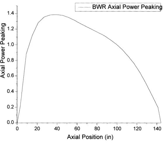
Axial power peaking
As axial power peaking we have used a single profile for the bundle extracted from the VIPRE manual. The profile represents the usual lower core peaking expected in a BWR core. The peak to average axial power value is 1.39, as seen in Figure 3.2.
1.4
12
.'- 1.2 L 1.0 a) L 0.8 X< 0.6
0.4 0.2 0.0 0 20 40 60 80 100 120 140Axial Position (in)
Figure 3.2: Solid fuel axial power peaking
I - - .- . . . - . . I
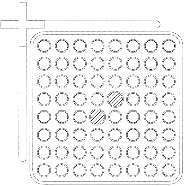
Radial power peaking
To obtain a representative radial power peaking, MCNP was used to model a bundle to obtain representative values. Figure 3.3 summarizes the pin peaking factors within the bundle. The actual calculation of this peaking will not be addressed in this report. The details can be found in [8].
0.994 1.016 1.073 1.112 1.113 1.074 1.016 0.993 0.355 0.995 1.086 1.090 1.000 0.36 1.015 0.996 1.010 1.038 1.013 0.999 1.072 1.070 0.000 1.038 1.089 1.111 1.069 1.009 1.084 1.110 0.995 0.993 1.071 0.355 1.013 0.991
Figure 3.3: BWR-5 8x8 radial power peaking
Core pressure drop
We don't have access to data about the local core pressure drops such as at grids, the entrance and the exit. We extracted it from the VIPRE manual sample input as said above. The data we were able to get are summarized in Table 3.3
Table 3.3: Local pressure drop coefficients
Location Coefficient
Orifice (average bundle) 24.28
Orifice (hot bundle) 23.37
Entrance plate 6.63
Grids 1.5
Exit plate 1.46
We would like to comment in particular on the orifice coefficients. The lowest inlet pressure drop coefficient reported in the sample input for was taken as the hot bundle one while the one that gives the right inlet pressure drop (see Figure 4.4) is taken as the average bundle orifice pressure drop coefficient. This last one is also the most common in the core modeled by the sample input.
Materials
The materials that we need to define in the code for our VIPRE model are two, fuel and cladding. For the cladding we have taken the standard Zircalloy property table that has been used in the PWR case [1]. Although Zircalloy-2, the cladding material used in BWRs, differs from Zircalloy-4, the cladding material used in PWRs, the difference is very small in the properties that interest us, in particular the thermal ones. For the fuel we have used the uranium oxide properties from the same reference [1].
3.2 Annular fuel design
3.2.1 Criteria for the bundle design
The first step is to design a possible annular fuel lattice for BWR reactors to fit the same bundle side dimensions. This constraint is very important because it will assure that the annular fuel we design will have the possibility to be used even by existing BWRs. Also this constraint limits the possible lattice choices, since the annular fuel will have obviously to be of larger diameter than the solid fuel if we want to accommodate a reasonable volume of fuel in the bundle and keep a sufficiently large internal channel diameter. As for now, both the 5x5 and 6x6 lattices could be interesting for our research, while both a smaller and larger lattice would probably give either hydraulic problems (channels too small), mechanical problems (fretting) or thermal problems (surface area too small).
There are two fundamental parameters to be decided, and they will identify unambiguously the fuel design:
* The ratio between the internal diameter of the annular fuel pin and the hydraulic diameter of the solid fuel bundle internal channels.
* The ratio between the total fuel volume in the solid and the annular bundle.
After some checks on the possible configurations we decided to accept to have only 90% of the fuel present in the reference in our annular fuel bundle. This will allow better thermal hydraulic performance of the core and eliminate a degree of freedom of the design at the expense of the neutronics of the design. Also it is the same choice made in the PWR case [].
The following dimensions were taken to be the same for the annular and solid fuel bundles:
* We will keep the assembly side length equal to that of the solid for retrofittability, * Clad thickness the same as the reference solid fuel pin,
* Internal clad thickness the same as the external clad thickness, * Gap dimension and conductance the same as solid,
* Internal gap the same as external gap,
* Water rod modeled as if it was composed only by the external clad of a fuel rod and with the same thickness,
* Water rod outer diameter the same as the fuel rod,
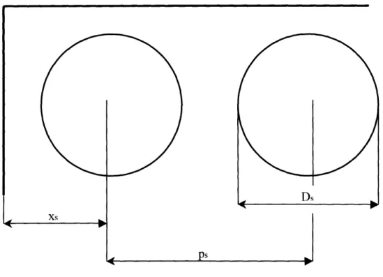
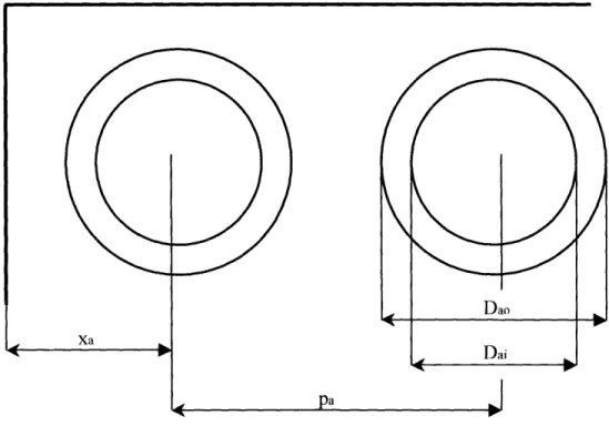
These assumptions and constraints are all based on thermal hydraulic, neutronic and vibrational considerations. In addition to these we need another constraint to get a unique solution given the above parameters. We chose to keep constant (at the same value as in the solid bundle) the ratio between the gap between rods and the gap between a corner rod and the bundle wall (_), this allows us to keep a reasonable ratio between the hydraulic diameters in various parts of the bundle.
Below we show a section of a solid (Figure 3.5) and an annular rod (Figure 3.4) and introduce the typical dimensions (Figures 3.6 and 3.7). The figures are not to scale.
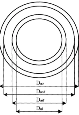
Figure 3.5: Annular fuel rod section Figure 34: Solid fuel rod section
Figure 3.7: Annular fuel rods layout in respect to the bundle wall
The procedure followed to design the annular fuel bundle is:
1. Choose the internal diameter of a pin
This is done indirectly choosing the ratio between the internal diameter of the annular fuel and the hydraulic diameter of the solid fuel
2. Calculate the external diameter of the annular fuel pin knowing the ratio between the total fuel in the solid and the annular bundles
where Na is the number of pins in the annular assembly (24 or 34) and Ns the number of pins in a solid assembly (62). The suffix 'f added to the geometrical parameters means that they are referred to the actual fuel within the pin.
3. Calculate the pitch of the annular fuel pins assuming that the ratio of the distance between the corner rod and the bundle wall and between the internal rods is the
same both for the annular and the solid fuel bundle:
where
The above assumption basically tries to keep the flow as similar as possible in the two designs.
With all the above assumptions, data and calculations the bundle is uniquely defined.
Also for the design to be accepted, it has to respect the following parameters:
1. The ratio between the internal diameter of the annular fuel and the hydraulic diameter of the solid fuel must be reasonable (between 0.7 and 1.1)
2. The distance of the corner rods from the wall and the distance between rods must be at least 1 mm
3. The moderator to fuel ratio of the annular fuel bundle must be close to the one of the solid fuel bundle (within 10%)
Every design that passes all the checks is considered viable and can be tested for the maximum power upgrade achievable.
3.2.2 Geometric data
We have explored many designs in the above illustrated parameters space. Here we will show only the ones that we considered more promising. The designs were chosen ultimately for their CPR performance but we had to take into consideration even the flow quality imbalance between the channels and other thermal hydraulic considerations. Also, we had to discard the designs for which the VIPRE code didn't converge for a reasonable number of axial nodes, since in that case we felt that we couldn't trust the code's CPR calculations.
3.2.2.1 The 5x5 bundle
On Tables 3.4 and 3.5 we show a comparative list of the important geometrical characteristics of the most promising designs.
Table 3.4: Annular fuel 5x5 possible designs
Internal Diameter
Fuel volume
Design (solid hydraulic Bundle lattice
(solid=100%) diameter=100%) Annular 1 100% 90% 5x5 Annular 2 90% 90% 5x5 Annular 3 85% 90% 5x5 Annular 4 80% 90% 5x5
Table 3.5: Geometrical parameters of the Annular fuel 5x5 possible designs
GE BWR/5 Annular 1 Annular 2 Annular 3 Annular 4
Bundle lattice 8x8 5x5 5x5 5x5 5x5 Number of fuel 62 24 24 24 24 rods Number of Water 2 1 1 1 1 rods Clad thickness (cm) 0.085 Gap (cm) 0.01 Inner distance
between box walls 13.4
(cm) Pellet OD (cm) 1.04 2.308 2.202 2.151 2.102 Pellet ID (cm) - 1.677 1.528 1.454 1.379 Fuel Rod OD (cm) 1.23 2.498 2.392 2.341 2.292 Fuel Rod ID (cm) - 1.487 1.338 1.264 1.189 Water Rod OD 1.50 2.498 2.392 2.341 2.292 (cm) Water Rod ID (cm) 1.32 2.318 2.212 2.161 2.112 Corner Hydraulic 1 C e1.010 0.632 0.811 0.897 0.980 Diameter (cm) Border Hydraulic Diameter 1.210 0.775 0.972 1.068 1.163 (cm) External Hydraulic Diameter 1.487 1.072 1.281 1.385 1.489 (cm) Internal Hydraulic Diameter - 1.487 1.338 1.264 1.189 (cm)
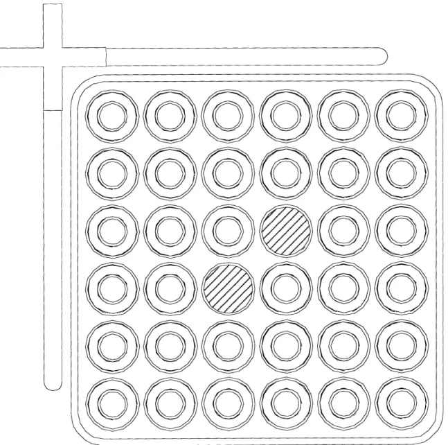
These are the most promising 5x5 designs. Annular 1 was discarded because it showed a large imbalance of flow qualities between the internal and external channels and in addition is slightly out of range of the tolerance we fixed for the fuel/moderator ratio. We discarded Annular 4 due to poor code convergence for this design. We chose the Annular 2 design due to better CPR performance compared to the Annular 3 design. From now on we will consider Annular 2 as the reference 5x5 annular bundle, and we show in Figure 3.8 below a possible 2D section of the bundle.
3.2.2.2 The 6x6 bundle
For the 6x6 bundle case there is less freedom in the design, since this design presents a more tightly packed bundle. This is due to the fact that we have now to fit 44% more rods than the 5x5 design in the same area, in order to keep the important feature of being able to use this fuel in existing BWR plants.
As described before in Section 3.2.1 we have many constraints in the design, so we cannot vary the internal diameter too much without either losing a good moderator to fuel ratio or placing the rods too close and thus risking vibration problems. As a consequence there is a smaller range of designs that respect all the constraints than the 5x5 bundle. Two designs have been chosen with parameters described in Tables 3.6 and 3.7 and Figure 3.9 shows a possible 2D section of the 6x6 bundle.
The Annular 5 design actually gives better thermal hydraulic characteristics and more open channels over the other candidate (Annular 6). Additionally it achieves a slightly better pressure drop for the same reason, and thus it is our selected design.
Table 3.6: Annular fuel 6x6 possible designs
Internal Diameter
Fuel volume
Design (solid hydraulic Bundle lattice
(solid-100%) diameter= 100%)
Annular 5 80% 90% 6x6
Table 3.7: Geometrical parameters of the Annular fuel 6x6 possible designs
GE BWR/5 Annular 5 Annular 6
Bundle lattice 8x8 6x6 6x6
Number of fuel rods 62 36 36
Number of Water rods 2 2 2
Clad thickness (cm) 0.085
Gap (cm) 0.01
Inner distance between box walls
13.4 (cm) Pellet OD (cm) 1.04 1.918 1.865 Pellet ID (cm) - 1.379 1.305 Fuel Rod OD (cm) 1.23 2.108 2.055 Fuel Rod ID (cm) - 1.189 1.115 Water Rod OD (cm) 1.50 2.108 2.055 Water Rod ID (cm) 1.32 1.928 1.875 Spacing rod-rod (cm) 0.390 0.106 0.150
Spacing rod-bundle wall (cm) 0.415 0.112 0.160
Lattice pin pitch (cm) 1.62 2.213 2.205
Corner Hydraulic Diameter (cm) 1.010 0.490 0.582
Border
Hydraulic Diameter 1.210 0.606 0.706
(cm)
External Hydraulic Diameter
1.487 0.852 0.958
(cm)
Internal Hydraulic Diameter
- 1.189 1.115
3.2.3 Other data
Axial power peaking
We have chosen to use the same axial power profile as the solid fuel case.
Radial power peaking
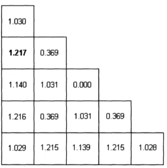
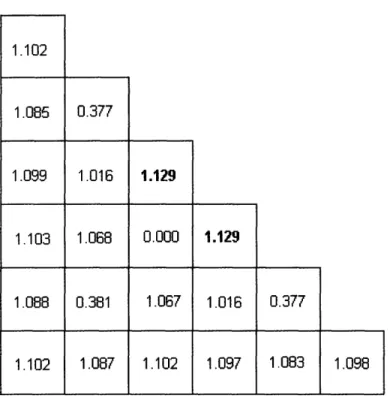
For this case the data were obtained from a MCNP model since there are no experimental data available for annular fuel. The actual calculation of this peaking will not be addressed in this report, but can be found in [8]. The radial power peaking used is shown in Figure 3.10() for the 5x5 bundle and in Figure 3.11 for the 6x6 bundle.
1.030 1.217 1.140 1.216 1.029 0.369 1.031 0.369 1.215 0.000 1.031 1.139 0.369 1.215 1.028
Figure 3.10: Radial power peaking for the 5x5 annular fuel bundle
-1.102 1.085 1.099 1.103 1.088 1.102 0.377 1.016 1.068 0.381 1.087 1.129 0.000 1.067 1.102 1.129 1.016 1.097 0.377 1.083 1.098
Figure 3.11: Radial power peaking for the 6x6 annular fuel bundle
Core pressure drop
We investigated the pressure drop for annular fuel. From preliminary calculations we have seen that for most designs the limiting factor is the quality imbalance between the inner and outer channels, due to the fact that those do not communicate. We can force more flow into the internal channel, and thus address this problem, in two ways: by enlarging the internal channel diameter (and thus changing design) or by increasing the grid pressure drop.
The technique we adopted consists of exploring all the parameters space. For a specific design (and thus an internal channel diameter), we progressively increased the grid pressure drop to force more flow in the internal channel. This allowed us to maximize the CPR for each design considered at the expense of the core pressure drop.
Materials
To allow a more precise comparison between annular and solid fuel bundles, the material properties of both the cladding and the fuel itself were kept the same as in the reference design.
3.3 Differences between the 5x5 and the 6x6 design
The 5x5 bundle allows more freedom in choosing the geometrical parameters due to the fact that we can fit 25 rods in the bundle in more ways than we can fit 36. This leads to larger hydraulic diameters and lower pressure drops. On the other side this 5x5 design does not increase much the heat transfer surface and has other constraints from the neutronic point of view, since we can adjust the burnable poison in very few rods.
A comparison between some geometrical parameters of the best 5x5 and 6x6 designs chosen for future analysis is given in Table 3.8 below:
Table 3.8: Comparison between the 5x5 and the 6x6 annular designs
GE BWR/5 Annular 5x5 Annular 6x6 Fuel to Moderator
volumetric ratio 1.000 0.889 0.955
(normalized)
Fuel Volume (normalized) 1.00 0.900 0.900
Moderator Volume 1.00 1.012 0.942 (normalized) Cladding Volume
Clddn V1.00
1.269
1.606
(normalized)Heated surface/fuel volume
1.00 1.304 1.633
(normalized)
We want to underline the fact that the moderator volume is thus the normalized flow area would give the same result volume.
proportional to the flow area, as the normalized moderator
As we can see the 6x6 annular fuel bundle shows a remarkably higher heated surface than the 5x5 design. Thus it is more promising for the goal of this work, the power uprate of
BWR nuclear power plants. Also it shows a closer moderator to fuel ratio to the reference and thus it has potentially better neutronics, or at least closer to the solid fuel's. We see that we pay for those improvements with the higher amount of cladding in the fuel and higher pressure drop (in the 6x6 case) due to the smaller flow area and larger surface area, as given in Table 4.2 in the next chapter.
Chapter 4: Results and Analysis
4.1 Validation of the model
First of all we want to validate the method we used by showing agreement of the reference data in literature with our solid fuel model. As discussed in Chapter 2 we will compare our single bundle output obtained using the VIPRE code with the data available in the open literature for BWR cores.
It is difficult to base our model on BWR fuel operating and limiting thermal conditions in a particular plant, both because the data is proprietary and because of the variability of the BWR cores built. So, we will use as reference typical range of values. Most of the reference data we select is obtained from reference [9].
4.1.1 Void fraction
Axial distributions of quality and void fraction for a typical BWR [6] are shown in Figure
4.1
0 0.1 0.2 0.3 0.4 0.5 0.6 0.7 0.8 0.9 1.0
Fractional Height
P13 cy
Figure 4.1: Void fraction and quality in a typical BWR 191
0.7
0.6
0.5
0.4 0.30.2
0.1
0
,::::i
Void-
F:a-;iin
ti
!i
n:::
c::
:h
-v!:t
I' C~ I}-." , iL,. . Q. .4 u.J of .:-- X; 0.'2: ... .. ,. . - : * . . . > . ., .. . . . .... .. . ...&, i,-'.- :.i'n::.
.- .. ADD. . - w-. . . .- .- A; . . - . . ; .. . .. .;. ; .- . . :; 0 .S : ; -: : :::-n :'n. 1Q .O
~1
0 6Figure 4.2: Void fraction in the solid fuel model
The results calculated with our model for the solid fuel are shown in Figures 4.2 and 4.3. As we can see in Figure 4.2 the plane averaged exit void fraction for the average bundle of the solid fuel calculated by VIPRE is 67%, which agrees very well with the reference value for the whole core 70%. Also the calculated axial average is 38.66% again for the average bundle while the reference core average is 40%. %. As a reminder, the heated section in the channel extends from position 13.5 inches to 157.5 inches.
I I I I I I I I I I I I I I 7 ._ I-_ L t Oi:!!, I I , .~L
4.1.2 Quality
We can see in Figure 4.3 below the equilibrium quality calculated with our solid fuel model 016 0.14 0.12 0.1 3 a.08 'U 0406 0.04 0.02 .n,
Quality in the average bundle
,,! ,., .2 ~ ~ ~ ~ ~ . A~~~~. .. ,,, I , , | , ^ . . .~~~~~~~~~../... I :Z: ::n:¢W 130 t~ll-- f;;- lD: tI:: 1
n--. S-'''0''""-;'Axil Ditance (inheh"'',-,-.: :) '
180
Figure 4.3: Equilibrium quality in the solid fuel model
From Figure 4.3, the plane averaged exit quality for the average bundle of the solid fuel calculated by VIPRE is 14.2%, again a value that agrees very well with the whole core average of 15%/o given by the reference.
.
20
;,:-e O~:35'. 'Z::;:? ' l : : ' : :
?
-W~i
IN0 ~ ~ ~ ~ ~ ~ ~ ~ ~~~~~4,XI'-.\X, ~ ~ ~
'"'.'d.025"',lSf'
Figure 4.4: Quality in the hot channel of the solid fuel model
Figure 4.4 shows the axial quality profile of the hottest channel in the core. We can see that the exit quality reaches 32%, about double that of the average. The hottest channel in this case is the side channel adjacent to the hot rod (see Figure 3.3). Since in our model the corner and side channels are smaller than the internal channels, those are the most likely to reach the highest quality. So, if the hot rod is also in conact with a corner or border channel this will probably become the hottest, like what happened in this case.
Also for the way VIPRE models the bundle we could have shown four channels around the hot rod. Here we have decided to show only the one that reaches the highest exit quality. The other channels in contact with the hot rod reach exit quality level 7% (relative value) lower at the most and thus are very close to the channel shown.
60
. ~ ~
~
0
04
0.
0\
0.7
08
0.
1 <
iiU
Figure 4.4: Quality in the hot channel of the solid fuel model
Figure 4.4 shows the axial quality profile of the hottest channel in the core. We can see that the exit quality reaches 32%, about double that of the average. The hottest channel in this case is the side channel adjacent to the hot rod (see Figure 3.3). Since in our model the corner and side channels are smaller than the internal channels, those are the most likely to reach the highest quality. So, if the hot rod is also in contact with a corner or border channel this will probably become the hottest, like what happened in this case.
Also for the way VIPRE models the bundle we could have shown four channels around the hot rod. Here we have decided to show only the one that reaches the highest exit
quality. The other channels in contact with the hot rod reach exit quality level 7% (relative value) lower at the most and thus are very close to the channel shown.
4.1.3 Pressure drop
We now compare the pressure drop shown in Figure 4.4 for a typical BWR [9] with the calculated pressure drop in the average bundle shown in Figure 4.5
& 8 -I
PressAure Drop (psi) o,,a
Figure 4.5: Pressure drop in a typical BWR 191
0 ~Z 0W A ~a sZ
I
0 (40
0 0z -=Pssur Prop in the averge bwdI I U Q 0
gaB
0 Q C 0 c p ' '5:-' ' : -: ..,'-, ' "'.''; '',''R.'S;' -:, A- . ,' , - h . , - , . .. ' i , ' ' ', ; " AS ' .' . ' ':''': A:-' ' :' ', ,,- l 1'. - . no ., . Lo L ,, I.. ,' O I0 15Z
253
0t
, ' , ; , , .Figure 4.6: Pressure drop in the solid fuel model
Again we can see the good agreement between the data. Our calculated core pressure drop is 21.6 psia, about the same value given in reference [9].
I I I - X ~~~~~~~~~~~~~~J I i f'2 I / i I I I -II I, L, , , : 11 , il ,L:",-'"-,-, 1;
4.1.4 MCPR
Reference [911 shows an indicative table for the Minimum Critical Power Ratio (MCPR) in BWR reactors. This is a key parameter since we intend to compare the performance of our annular uel to the solid fuel on the basis of this quantity. Also this parameter is closely related to the safety of the reactor since if MCPR<1 then by definition we will encounter a thermal crisis (dryout) somewhere in the reactor with subsequent damage of the fuel and possible release of radioactive material in the primary loop, as discussed in Chapter 2. This is especially undesirable in BWR reactors since part of the coolant goes directly in the turbine and thus is present even outside the containment.
It is not enough to keep the MCPR just above one, since we have to allow a margin for uncertainties, transients and operation.
AMCPR 1.30+ 1.23 1.06 1.00
t
OperatlnI MarginMargin for Transients
Margin for Lkcertanties
t
Normal Operation Steady-State Operating Limit (CLMCPR Safety Limit Data BaseFigure 4.7: MCPR in a typical BWR reactor
As we can see from Figure 4.7 the MCPR must be 1.30+. There are studies about the possibility to operate with lower MCPR, between 1.2 and 1.26, but we are working with
It is more demanding to validate our results for the MCPR since they show a dependence on the number of axial nodes used to model the bundle.
VIPRE is a computer code and thus it relies on its ability to compute the solution of the original system of differential equation that describes the physical reality by discretizing it. The differential equations are transformed in finite differences so that they can be solved using the high computational power of the computer. This discretization applies to all variables but is especially evident for the spatial ones (and time, in transients). To be able to use the discrete model, the code has to divide space in meshes and it concentrates the variables that apply to a mesh in its center, the node (usually).
VIPRE allows the user to choose the number of axial nodes to model his system. Usually using a very low number of axial nodes is not recommended since a coarse mesh means smearing over variation within each node and more errors in the solution of the system, because the code would lump too many different zones together. Also a very fine mesh is usually not a good idea since it increases the computational time and memory needs. Furthermore, it eventually will arrive to a point where other errors will become more important than the ones related to discretization and thus the result will not be improved any more by refining the mesh. Also, there may be internal limits depending on the code in use.
So, there is usually a window of mesh sizes that should be used and if the code is reliable the results obtained for all these possible values should be consistent in the sense that there should be a steady refining of the result toward the 'true value'. By the nature of the discretization process we understand that the finer the mesh the closer we should be to the 'true value', provided that the limits of the code have not been exceeded or other errors become more important.
As seen in Figure 4.8, we get a reasonably good convergence toward a value as we increase the number of axial nodes, but we didn't achieve convergence for all the possible numbers of axial nodes in our 'mesh window'.
I
.
IA
$
..
IA
'pDr
"
1.60-1 .55-1.50-0
a-1.45- 1.40- 1.35- 1.30-1.25- I , I I 11 II I 1 I I I 20 40 60 80 100 120 140 160 Axial nodesFigure 4.8: MCPR in the solid fuel model
Even if we didn't achieve convergence for all the possible values of axial nodes, it is already evident that the MCPR is converging toward a definite value, around 1.3.
We can easily show that by plotting a 10% error band (see Figure 4.9):
ior
Solid fuel MCPR
10% error bar
I I I I lI I I I ' I I 40 60 80 100 120 140 160
Axial Nodes
Figure 4.9: MCPR comparison with reference (10% error bar) 1.60 - 1.55- 1.50-1.45= .40 1.35- 1.30-1.25 1.20= -1 -IR 20 1--1 , ..J
Also, if we look only to the higher number of axial nodes, we can see from Figure 4.10 that all the results are inside a 5% error from the suggested value of 1.3, thus
strengthening our belief that the code is actually converging to that.
1 1 1 . r 20 40 60 80 100 Axial Nodes 120 140 160
Figure 4.10: MCPR comparison with reference (5% error bar)
The results we show look reasonable, since the oscillation for the smaller number of axial nodes shows that the calculation with a coarse mesh is not precise enough. With a finer mesh we get values that are very close to each other and definitively inside the error band we would expect from the correlation. We also achieved relative convergence on almost
Solid fuel MCPR error ba m4 n1 0 1 1 1 1 .. _ _ _ . . .. T T 7-I i i \ i -16 00 -I i ; - -L
We stopped at 160 axial nodes for computational time reasons and because we think that in a system like ours it is meaningless to use even a higher number, not for an internal limit of the code.