Design and analysis of kinematic couplings for modular machine and instrument structures

Design and Analysis of Kinematic Couplings for

Modular Machine and Instrumentation Structures

by

Anastasios John Hart

B.S.E. Mechanical Engineering (2000)

University of Michigan

Submitted to the Department of Mechanical Engineering

in partial fulfillment of the requirements for the degree of

Master of Science (S.M.)

at the

MASSACHUSETTS INSTITUTE OF TECHNOLOGY

FEBRUARY 2002

© Massachusetts Institute of Technology, 2002. All Rights Reserved.

A u th or ...

Department of Mechanical Engineering

December 10, 2001

Certified

lexander H. Slocum

Professor of Mechanical Engineering

Thesis Supervisor

A ccepted by ...

Chairman,

Ain A. Sonin

MechanicalEpgineering Graduate Committee

MASSACHUSETTS INS I ILU

OF TECHNOLOGY

MIlUmenbrries

Document Services

DISCLAIM ER

Page has been ommitted due to a pagination error

by the author.

Design and Analysis of Kinematic Couplings for

Modular Machine and Instrumentation Structures

by

Anastasios John Hart

Precision Engineering Research Group

Massachusetts Institute of Technology

Submitted to the Department of Mechanical Engineering on

December 10, 2001 in partial fulfillment of the requirements for the

degree of Master of Science

Abstract

For decades, kinematic couplings have been developed and used because of their

astound-ing repeatability, but few efforts have been made to unify the design theory into a general

strategy for widespread application of deterministic interfaces in flexible automation,

where both repeatability and interchangeability are important. Accordingly, this thesis

seeks to present a methodology for using kinematic couplings as deterministic interfaces

for modular machine and instrumentation structures, with focus applications to design of

an industrial robot factory interface and design of a next-generation microscope structure.

Theory is presented for design of traditional ball/groove, canoe ball, traditional

quasi-kinematic, three-pin quasi-quasi-kinematic, and cylinder/groove quasi-kinematic couplings.

Furthermore, the ability to parametrize kinematic coupling performance is extended from

reliance on experimental repeatability analysis to an estimate of Total Mechanical

Accu-racy, based on a closed-form computer model for determining the interchangeability of

canoe ball and three-pin interfaces. With calibration of the interface by measurement of

the perturbed locations of its contact points, introduction of an interface transformation to

a machine's structural loop can reduce the deterministic interchangeability error to

essen-tially that inherent in the routine of the measurement system used for calibration. Perhaps

more powerfully, a parametric model of interchangeability allows engineers to predict the

accuracy of an interface, based on tolerance distribution parameters assigned to the

cou-pling manufacturing process, plate manufacturing process, interface assembly process,

and interface calibration process. This predictive ability enables choice of manufacturing

process precision and calibration detail to give the desired interface accuracy at minimum

cost. Modularity of structures based on kinematic couplings can also be exploited to

pro-vide flexibility through being able to interchange style-specific manufacturing tools

with-out the need for re-calibration of machines, and as demonstrated by the microscope case

study, significantly improved thermal performance for ultra high-precision applications.

Looking forward, the ability to characterize performance of kinematic couplings in a

closed form makes them well-suited for development of a standard representation for

kinematic couplings. Most powerfully, kinematic couplings can be envisioned as an ideal

handshake between precision mechanics and information technology. At the most basic

level, encoding of interface calibration data on a wireless tag can initiate communication

between the interface and a calibration computer when the interface is in proximity to the

machine. A conceptual framework for further thinking in convergence of quick-change

interfaces and thin-client information interfaces to build low-cost, intelligent, flexible,

automation processes, is given.

Thesis Supervisor: Alexander H. Slocum

Table of Contents

1. Introduction

13

1.1 Motivation 13

1.2 Deterministic Systems 15

1.3 Thesis Outline 16

2. Kinematic Coupling Design

19

2.1 Traditional Kinematic Couplings and Fundamental Design Theory 19

2.2 Canoe Ball Couplings 26

2.3 Quasi-Kinematic Couplings 27

2.4 Three-Pin In-Plane Coupling 30

2.5 Fatigue Life Considerations 35

2.6 Interface Packaging and Tightening Torque Specification 36

3. Interchangeability of Deterministic Kinematic Interfaces

39

3.1 Repeatability vs. Interchangeability 39

3.2 Global Error Model of a Kinematic Coupling Interface 40

3.3 Kinematic Coupling Measurement and Calibration 47

3.4 Applied Modeling of Error Components 57

3.5 Parametric Relationship of Calibration Detail vs. Mating Accuracy 64

3.6 Bench-Level Interchangeability Model 72

3.7 Interchangeability Model of Three-Pin Interface 78

3.8 A New, Interface-Driven Machine Module Calibration Process 81

3.9 Conclusions and Future Work Plans 83

4. Machine Case Study: Mechanical Performance of a Quick-Change

Industrial Robot Factory Interface

87

4.1 Background and Problem Definition 87

4.2 Current Interface Design and Robot Installation Procedure 91

4.3 Customer Attitudes Towards Interface-Based Modularity 94

4.4 Quick-Change Interface: Applied Kinematic Coupling Design Process 96

4.5 Prototype Repeatability Tests 113

4.6 Factory Interface Interchangeability Simulations 128

4.7 Conceptual Extension to Four-Point Mounting 136

4.8 Improvements to Robot Accuracy 137

4.9 Caveats and Needs for Future Work 140

5.

Instrumentation Case Study: Thermal Performance of a Modular

Structure for a High-Precision Microscope

143

5.1 Overview of the High Precision Microscope Project 143

5.2 Design and Theoretical Basis of the Modular Structure 145

5.3 Thermal Stability Evaluation 153

6. Toward Standard, Low-Cost, Intelligent, Modular Systems

187

6.1 The Interface Design Process 187

6.2 Fundamental Hardware and Software 193

6.3 Intelligent Manufacturing Systems Using Kinematic Couplings 203

7. Conclusion

₂₁₃

8. Appendices

₂₁₅

A. References 215

B. Kinematic Coupling Design Code 217

B. 1 Design of Traditional and Canoe Ball Couplings 217

B.2 Contact Force Calculation for Three-Pin Interface 229

B.3 In-Plane Preload Calculation (Friction Limit) for Three-Pin Interface 230

B.4 Bolt Tightening Torque Calculation 235

C. Kinematic Exchangeability Analysis Code 237

C. 1 Canoe Ball Interface Exchangeability 237

C.2 Three-Pin Interface Exchangeability 252

C.3 Common Routines, Used By Both Simulations 255

D. Appended Thermal Stability Results 257

List of Figures

Chapter 1

1.1 Summary of kinematic and quasi-kinematic interface designs. 14

1.2 Schematic of an intelligent kinematic interface. 16

Chapter 2

2.1 Model of three-ball/three-groove kinematic coupling (with magnetic preload). 20 2.2 Planar triangular kinematic coupling layout showing coupling centroid [4]. 21

2.3 Canoe ball mount with 250 mm contact surface radii. 26

2.4 Typical quasi-kinematic coupling interface. 28

2.5 Quasi-kinematic contactor. 29

2.6 Quasi-kinematic target with 9c7= 90 deg. 29

2.7 Arrangement of three-pin interface. 31

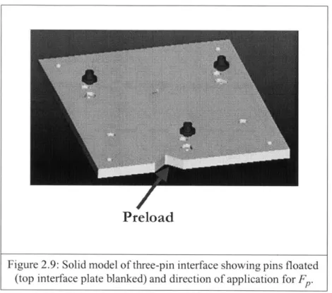
2.8 In-plane preload and contact reaction forces against three-pin interface. 32 2.9 Solid model of three-pin interface showing pins floated (top interface plate blanked) and

direction of application for F.

Chapter 3

3.1 Modular machine interface with kinematic couplings, designating reference interface, tool, and

measurement system coordinate frames. 41

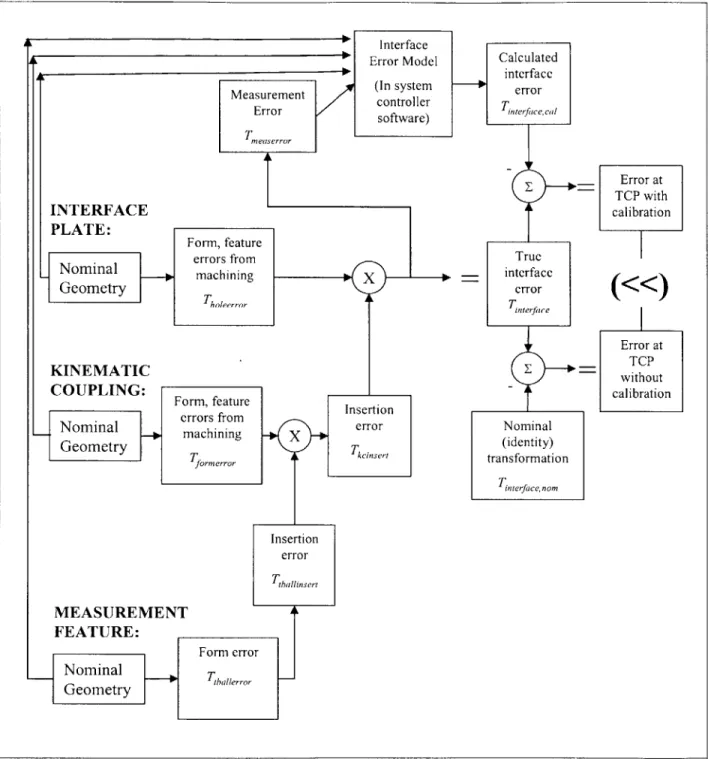
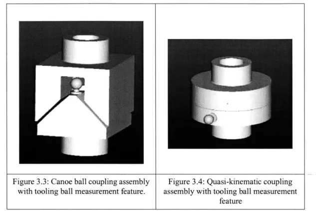
3.2 Block diagram representation of the error stackup for a kinematic coupling interface. 45 3.3 Canoe ball coupling assembly with tooling ball measurement feature. 48 3.4 Quasi-kinematic coupling assembly with tooling ball measurement feature 48

3.5 Canoe ball mount with integrally machined measurement hemisphere. 49

3.6 In-plane depiction error motion due to perturbations in ball and groove positions and

orientations. 54

3.7 Ball error components in local x-direction. 60

3.8 Ball error components in local y-direction. 61

3.9 Ball error components in local z-direction. 62

3.10 Structure of MATLAB model for parametric error analysis of canoe ball interface. 68 3.11 Tool point error versus interface calibration detail -calibration using offset measurement

sphere. 71

3.12 Tool point error versus interface calibration detail -calibration using direct measurement of

ball and groove contact surfaces. 71

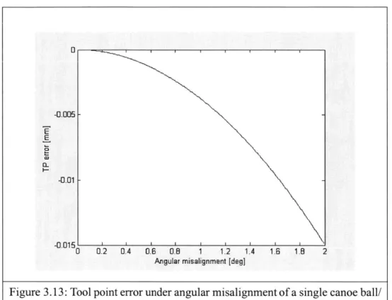
3.13 Tool point error under angular misalignment of a single canoe ball/groove pair. 72 3.14 Prototype groove base for measurement of canoe ball interface interchangeability (three

adjacent grooves removed). 73

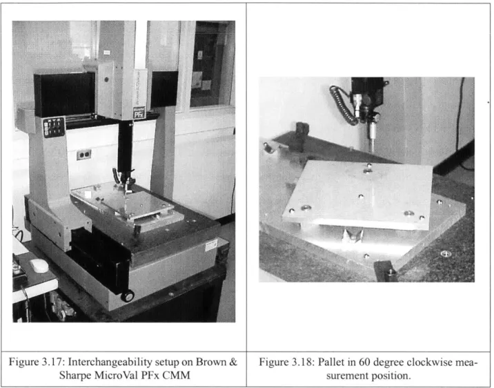
3.15 Prototype pallet for interchangeability measurements -canoe ball side. 73 3.16 Prototype pallet for interchangeability measurements -measurement sphere side. 73 3.17 Interchangeability setup on Brown & Sharpe MicroVal PFx CMM 75

3.18 Pallet in 60 degree clockwise measurement position. 75

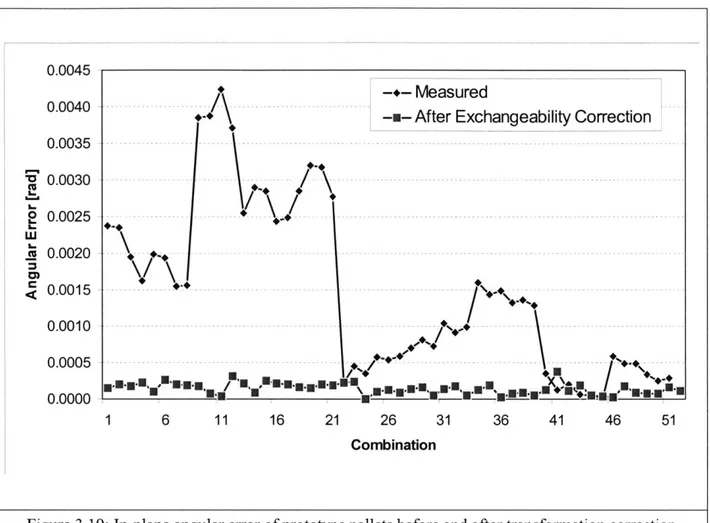
3.19 In-plane angular error of prototype pallets before and after transformation correction. 77 3.20 Simple ball interface calibration to workcell using ball bar. 82

Chapter 4

4.1 Six-axis industrial robot manipulator commonly used in automotive assembly (ABB

IRB6400R). 88

4.2 Nomenclature of ABB IRB6400R's six revolute axes [1]. 88

4.3 Three-point manipulator foot (ABB IRB6400). 92

4.4 Schematic of four-point manipulator foot (ABB IRB6400R) [1]. 92 4.5 Four point, eight-bolt 6400R manipulator foot mounted on test pallet. 92 4.6 Scale prototype canoe coupling interface, with 3/4-scale placement relative to the full-size

design. 97

4.7 Tooling ball reference sphere. 98

4.8 Leica laser tracker with retro-reflector in calibration seat. 98 4.9 Prototype steel interface plate to manipulator foot -top side. 100 4.10 Prototype steel interface plate to manipulator foot -bottom side. 100 4.11 Prototype steel interface plate to manipulator foot -top side. 100 4.12 Solid model of interface assembly for static stress analysis. 101 4.13 Deformation of prototype interface assembly under fully-reversed operation loading. 102 4.14 Canoe groove fitted to top interface plate, showing secondary alignment pin. 104 4.15 Canoe ball with integrated tooling ball fitted to bottom interface plate. 104

4.16 Interface plates fitted with canoe ball couplings. 105

4.17 Mounted canoe ball joint with tooling ball. 105

4.18 Prototype shouldered coupling pin -side view. 107

4.19 Prototype shouldered coupling pin -perspective view. 107 4.20 Application of preload through threaded hole in floor interface plate. 107

4.21 Preload screw in prototype floor interface plate. 107

4.22 Shoulder pin fitted to top interface plate. 108

4.23 Interface plates fitted with three-pin couplings. 108

4.24 Mounted three-pin joint. 108

4.25 Flanged mild steel groove. 110

4.26 Aluminum cylinder mounted statically between pair of grooves. 110 4.27 Solid model of quasi-kinematic coupling assembly with measurement ball. 112

4.28 Solid model of prototype quasi-kinematic contactor 112

4.29 Solid model of prototype quasi-kinematic target. 112

4.30 Cell setup for repeatability measurements, showing mounted manipulator in crouched home

position and laser tracker. 114

4.31 Leica cat's eye retroreflector mounted on robot tool flange. 114 4.32 Manipulator harnessed to crane, hanging unbolted over floor interface. 116 4.33 Retroflector seated in measurement hole in top interface plate. 116

4.34 Programmed measurement path -point 1. 117

4.35 Programmed measurement path -point 2. 117

4.36 Programmed measurement path -point 5. 118

4.37 Programmed measurement path -point 3. 118

4.38 Programmed measurement path - point 4. 118

4.39 Progressive average measurement distances from previous trials for interfaces. 121 4.40 Comparison of average relative repeatabilities to performance of current two-pin base. 122 4.41 Cartesian TCP deviations from first trial -three-pin interface, refined mounting. 124 4.42 Cartesian TCP deviations from first trial -canoe ball interface, refined mounting. 125 4.43 Cartesian TCP deviations from first trial -groove-cylinder interface, refined mounting. 126

4.44 Canoe ball surface after eleven base mountings. 127

4.46 Parametric calibration complexity vs. interchangeability relationship for canoe-ball manipulator base interface: offset measurement, low measurement system error, varying

form error. 131

4.47 Parametric calibration complexity vs. interchangeability relationship for canoe-ball manipulator base interface: direct measurement, low measurement system error, varying

form error. 132

4.48 Calibration complexity vs. interchangeability relationship for three-pin interface. 135 4.49 Split groove canoe ball to accommodate kinematic mounting using all four corners of a bolt

rectangle. 137

4.50 Four-point coupling locations on four-corner mounting base. 137

Chapter

5

5.1 Cross-section of High-Precision Microscope (HPM) concept model. 144

5.2 Exploded model of segmented structure including two canoe ball sets. 147

5.3 Close view of canoe ball interfaces between segments. 147

5.4 Theorized constant temperature profiles on tall and short cylindrical tubes. 149

5.5 Temperature sensor placements and nomenclature. 154

5.6 Optical beam path and laser metrology setup. 156

5.7 DPMI assembly on 5" diameter central reference column. 156

5.8 Final test assembly -segmented structure. 157

5.9 Final test assembly -one-piece control structure. 157

5.10 Thermal isolation chamber. 158

5.11 Solid model of segmented structure for finite element simulation. 160

5.12 Solid model of one-piece control structure for finite element simulation. 160

5.13 Steady-state temperature contours on segmented model. 161

5.14 Steady-state temperature contours on one-piece model. 162

5.15 Axial displacement contours on segmented tube model. 163

5.16 Axial displacement contours on one-piece tube model. 163

5.17 Deflection of segmented structure versus time (measurement duration extended to 13 hours to

show thermal relaxation). 165

5.18 Comparison of deflections of segmented and one-piece structures over 450-minute test. 166 5.19 Normalized temperatures (10-minute averages) around tube 1 (non-heated) of segmented

structure. 167

5.20 End-to-end normalized temperature difference on tube 1 of segmented structure. 168 5.21 Normalized temperatures (10-minute average) around tube 3 of segmented structure. 169 5.22 End-to-end normalized temperature difference on tube 3 of segmented structure. 170 5.23 Circumferential normalized temperature profiles for tube 3 of segmented structure. 171 5.24 Normalized temperatures (10-minute average) around level 3 of one-piece structure. 172 5.25 End-to-end normalized temperature difference at level 3 of one-piece structure. 173 5.26 Comparison of measured and predicted angular deflections of segmented structure. 177 5.27 Axial displacement contours on copper (left) segmented structure. 179 5.28 Axial displacement contours on stainless steel (right) segmented structure. 179 5.29 Angular deflection of segmented and one-piece copper structures with varied thickness. 181 5.30 Angular deflection of structure with varying number of segments. 181 5.31 Angular deflection versus dimensionless segment length to thickness ratio. 182 5.32 Simulation model with insulation bonded to outside surfaces of tube segments. 183 5.33 Steady-state axial displacement contours on 1.5" insulation / 2.5" copper model. 183

Chapter 6

6.1 Parameter heirarchy for a canoe ball interface. 189

6.2 Isometric model view of extruded locator with central hole for clamping bolt. 196 6.3 End view of extruded locator in double mating vee grooves. 196

6.4 Section design parameters of extruded locator. 197

6.5 Non-deformed and deformed waterjet aluminum locators. 197

6.6 Aluminum locator clamped between vee grooves with side datum blocks on test fixture. 198 6.7 Communications architecture of a smart interface with locally-written parameters. 200 6.8 Communications architecture of a smart interface or module with server storage. 201 6.9 Integrated mechanical and information infrastructure for modular factory robotics. 205 6.10 Model of wireless measurement tool kinematically coupled to groove plate on body

subassembly welding fixture. 209

6.11 Ball-groove interface holding tool in non-contact evaluation of flange position. 210 6.12 Example wireless communication architecture between measurement unit, part, tool, and

List of Tables

Chapter 2

2.1 Fatigue strengths of selected steel alloys [12]. 36

Chapter 3

3.1 Representative 3-sigma values for interface error components. 64 3.2 Calibration options for canoe ball interface, using offset measurement feature. 66 3.3 Calibration options for canoe ball interface, directly measuring contact surfaces. 67 3.4 Error component values for parametric study with varied calibration complexity. 69 3.5 Canoe ball interface geometry for parametric study with varied calibration complexity. 69

3.6 Calibration options for three-pin interface. 80

Chapter 4

4.1 Manipulator exchange times under varying levels of on-line calibration. 95 4.2 ABB IRB6400R dynamic loads at center of foot (max, min). 96

4.3 Initial design parameters for canoe ball couplings 103

4.4 Final Specifications of prototype canoe ball coupling 104 4.5 Required preloads to pin interface in cases of partial contact. 106 4.6 Specifications of designed prototype quasi-kinematic couplings. 111 4.7 Average tool point path repeatabilities [mm] of current ABB and new kinematic coupling base

designs, relative to previous trials. 120

4.8 Average tool point path repeatabilities [mm] of current and new designs, relative to nominal

average of all trials. 123

4.9 Error component values for canoe ball interchangeability simulation. 129 4.10 Error component values for three-pin interchangeability simulation. 133 4.11 Total Mechanical Accuracy (TMA) of manipulator base solutions. 138

Chapter

5

5.1 Steady-state and transient performance index values for various metals. 151 5.2 Simulated and measured end-to-end circumferential temperature differences [C]. 174 5.3 Tube material optimization study results (DT = heated minus non-heated). 178

Chapter 6

Chapter 1

Introduction

1.1 Motivation

As budgetary and manufacturing quality requirements simultaneously become more stringent, manu-facturing strategies are focusing on modular machine systems as a means for achieving flexibility to pro-duce multiple products at flexible volumes, minimizing downtime in the case of catastrophic equipment failures, and maximizing reusability of machine modules between product generations. In modularizing machines to build these flexible systems, decisions regarding the degree to which machines should be seg-mented are often a trade-off against machine accuracy. For example, making a single, non-modular machine, such as an industrial robot, would require full calibration upon initial installation. When the machine fails, one must decide whether to repair the machine online, or replace it with an entirely new spare part. Replacement in this case almost always necessitates a re-calibration before production can be resumed.

One of the main contributors to the error of machine interchanges is the accuracy of the mounting interface, whereby the manufacturing errors in the interface locators, and the potentially non-deterministic nature of the interface contact itself, prevent installation with sufficient accuracy to eliminate the need for re-calibration of the machine. Kinematic couplings, researched and used for decades in large part because of their astounding repeatability, offer a potential solution to the problem of requiring re-calibration when new machine modules are installed. The near-exact constraint of the kinematic coupling relationship means that the error of interchange can be predicted if the positions of the coupling locators are known ahead of time. Hence, a correction for the interface mounting error is a virtual calibration routine in soft-ware, rather than a physical measurement routine when the new machine module is mounted into the man-ufacturing system. Furthermore, once modularity of machines can be achieved with minimum error of interchangeability, other mechanical benefits can be achieved, including ability to interchange style-spe-cific tooling components rapidly, give easier access for critical repairs, and thermally isolation of critical structural areas.

Over the past twenty years, research in kinematic couplings has extended the basic concepts of a tradi-tional coupling between three balls and three grooves, or between three cylinders and three grooves, to numerous variants of exact and near-exact constraint mountings. Figure 1.1 summarizes several common types of kinematic couplings, categorized in terms of their type of contact. Note that an increased level of determinism, e.g. 6-point contact versus line and/or surface contact, results in increasing stiffness and increasing repeatability.

6-Point Traditional KC: -Sphere size matched to groove

-Closed-form Hertz

contact solution for stresses + error motions -Measured repeatability -1 micron

Canoe Ball KC: -Oversized sphere, with "canoe" shaped ball mount

-10-100 times load capacity of traditional KC for same size groove

-Closed-form Hertz solution applicable -Measured repeatability -0.1 micron Line Quasi-kinematic: -Spherical contactors in conical targets -Approximate closed-form solution -Trivial to directly machine mating surfaces directly into parts

Cylinder/groove: -Three cylinders in three vee grooves

-Closed form approximation based on Hertz cylinder/line contact -Makes extruded locators possible

Line/Surface Three-pin:

-Three dowel pins into holes in opposite interface plate

-Quasi-kinematic in-plane mating by preload; vertical surface engagement between plates for stiffness

STIFFNESS

REPEATABILITY

Figure 1.1: Summary of kinematic and quasi-kinematic interface designs.

In seeking to extend the applicability of kinematic couplings and low-cost near-deterministic interfaces in general, to widespread industrial situations, a number of research questions must be answered:

1. How do performance parameters of kinematic couplings, such as stiffness and repeatability, change in applications involving extremely high loads?

2. How can the deterministic nature of kinematic couplings be exploited to not only provide astound-ing repeatability, but also very low error of interchangeability; and how can kinematic couplastound-ings be calibrated to minimize their interchangeability error?

3. Based on the answers to (1) and (2), can new types of kinematic couplings be designed to provide sufficient accuracy and repeatability for high-load industrial applications, at a significantly lower cost than existing designs?

4. Finally, how can kinematic couplings design, and use of modular machines in general, be made a closed-loop design process? Engineers should be able to predict the accuracy of their designs before mass-production; interfaces should automatically be recognized and calibrated upon installation to a machine; and performance parameters from a machine should automatically be archived and fed back to the designer so remote process control can be conducted.

This thesis provides preliminary answers to the above queries.

1.2 Deterministic Systems

Motivated by the concept of using kinematic couplings to remove the dependence of machine inter-changeability error on of mounting the module interfaces, deterministic interfaces are well-suited to a stan-dard mechanical design and information representation. Information is inherently deterministic, and object-oriented representations such as Java and XML improve extensibility of information, and make it easier to network components and define behaviors using standard protocols. Accordingly, kinematic cou-plings can be treated as deterministic mechanical and information objects, with their design parameters (e.g. interface type, material, etc.) and calibration parameters as member variables. As conceptualized in Figure 1.4, a memory tag on a kinematic coupling can note its calibration parameters, for recognition by a reader-equipped control cabinet upon installation to a machine.

The grand goal would be to develop an accepted standard for mechanical interchangeability among components, so the identification number on a kinematic interface not only gives the calibration parame-ters to the interface locators, but also gives a unique identifier to the module equipment itself. The identi-fier can be traced to a centralized database, where specific information about the module equipment is contained, such as geometrical data, manufacturing history, repair history, and additional calibration parameters.

Wireless Close Read OR Direct Entry -E 0 C o C# de/RFID) I CONTROL CABINET - Ethernet

---

Figure 1.2: Schematic of an intelligent kinematic interface.

The most apparent application of standardization is to robotics, for which the standards could enable a robotic subassembly, such as a wrist, to be easily changed, without requiring recalibration of the robot. The wrist would mate to a standard plate. A similar master plate would be located at the robot manufacturer, and each subassembly would be calibrated with respect to the mounting plate master. Thus when a replace-ment subassembly is delivered to the factory, it comes with a set of calibration coefficients with respect to the mounting plate master, and it can be "plugged into place and start working". Thus should a subassem-bly fail during use, it could be "unplugged" and a new subassemsubassem-bly could be "plugged in" and used

with-out having to recalibrate it to the line.

1.3 Thesis Outline

This thesis focuses on application of kinematic couplings to enable high-precision modularity of fac-tory automation, with two focus applications: the facfac-tory interface of a heavy-duty-industrial robot used for automotive body assembly, and the structure of a next-generation microscope to be used for single-molecule biological investigations. This document is organized as follows:

SERIA

Chapter 2 is an overview of the basic principles of kinematic coupling design and Hertzian contact mechanics. These principles are applied to present design methodologies for traditional ball/ groove, canoe ball/groove, three-pin, groove/cylinder, and quasi-kinematic couplings.

Chapter 3 presents and validates a deterministic model for assessing the interchangeability error of kinematic interfaces caused by assembly variation and form error in the coupling units and

inter-face mounting plates. The model is presented in detail as an exact solution for canoe ball cou-plings, and is extended with deterministic mating assumptions to the three-pin interface. Chapter 4 presents an application case study of canoe ball, three-pin, and groove-cylinder cou-plings to the factory interface of the ABB IRB6400R industrial robot manipulator. Results of static and dynamic repeatability measurements are presented, and the interchangeability of the canoe ball and three-pin designs is simulated using the model described in Chapter 3.

Chapter 5 presents the structural design of a modular high-precision microscope as a series of tube segments connected by canoe ball kinematic couplings. Experimental study and design optimiza-tion using finite element simulaoptimiza-tion show that the segmented design offers a significant thermal

stability advantage over a one-piece tubular structure, and the known high repeatability of the kinematic couplings enables the structural modules to be interchanged without recalibration of the optics.

Chapter 6 presents a framework for large-scale implementation of kinematic couplings in a modu-lar manufacturing system. Three developments would be critical: standardization of the kinematic coupling design process through a set of input and output parameters specific to each interface; design of low-cost locators with smart methods to hold interchangeability calibration parameter data; and integration of the interfaces into a networked system to enable 'plug-and-play' authenti-cation of interfaced parts or carriers and feedback of process performance data.

Chapter 2

Kinematic Coupling Design

A fundamental technology of high-precision mechanical interfaces for modular machine and instrumenta-tion structures is the kinematic coupling. This chapter provides a fundamental descripinstrumenta-tion of kinematic coupling design, with special considerations given to interfaces used in equipment that is subject to large disturbance forces. While traditional ball-groove kinematic couplings are a century-old design offering micron-level repeatability, developments of recent research have produced variants suited to special high-load, high-cycle, and high-volume installation applications, including the canoe ball coupling [1], the quasi-kinematic coupling [2], the three-tooth coupling [3], and most recently the three-pin coupling. For all such types, closed form relations or well-grounded approximations directly guide interface geometry design and material selection when the load case is known. This chapter presents contact mechanics theory applied to kinematic couplings, and briefly discusses design processes for traditional, canoe ball, quasi-kinematic, and three-pin interfaces.

2.1 Traditional Kinematic Couplings and Fundamental Design Theory

Kinematic couplings have been used for over a century as a method of precisely locating components of a mechanical assembly. The oldest, most common form is the three-ball/three-groove kinematic cou-pling shown schematically in Figure 2.1. The ball/groove coucou-pling matches a planar, triangular arrange-ment of three hemispheres on one component to three "vee-grooves" on another component. This match deterministically constrains all six degrees of freedom (DOF) -- three directions of translation and three directions of rotation -- between the components.

Figure 2.1: Model of three-ball/three-groove kinematic coupling (with magnetic preload).

The stability of a kinematic coupling interface is maximized when the coupling ball and groove cen-terlines, the normals to the planes containing pairs of contact force vectors, intersect at the centroid of the coupling triangle as shown in Figure 2.2. In other words, the centerlines bisect the angles of the coupling triangle, and intersect at a point called the coupling centroid. For static stability, the planes containing the pairs of contact force vectors must form a triangle [4]. Beyond this, in a specific case of extemal dynamic loading of the interface, stability is ensured by checking that none of the contact forces reverse from a compressive state, and applying a necessary preload to meet this condition.

Stiffness of a kinematic coupling is also related to the coupling layout. Stiffness is equal in all direc-tions when all the contact force vectors intersect the coupling plane at 45-degree angles. Coupling stiffness can be adjusted by changing the interior angles of the coupling triangle; elongating the triangle in one direction will increase the stiffness about an axis normal to the coupling plane and normal to the direction of elongation, and decrease the stiffness about an axis in the coupling plane and normal to the direction of

Ball 1 Groove 1

Coupling centroid _{Coupling triangle}

Angle bisector between sides 23 and 31 Ball 2 Ball 3 Plane containing the contact force vectors

Figure 2.2: Planar triangular kinematic coupling layout showing cou-pling centroid [4].

Traditionally, kinematic coupling performance is characterized in terms of repeatability versus applied load and the number of interface engagement cycles. Repeatability depends upon several factors including the coupling material and geometry, the preload and the working load, the number of coupling cycles, and the coupling surface finish and its exposure to debris. Hence, repeatability is almost exclusively an experi-mentally-defined parameter. At high numbers of cycles, fretting corrosion between plain steel surfaces can degrade repeatability; hence, non-corroding materials are best for use in high-cycle applications [4].

Most recently, Hale has presented computational models for predicting repeatability of a coupling interface, parametrized by groove angle and coefficient of friction between the balls and grooves [5]. Max-well's criterion is applied to determine the sensitive sliding direction for a coupling layout, and the fric-tional non-repeatability is predicted for when an interface is assembled imperfectly and is stopped short of its nominal seating position by interfacial resistance between the balls and grooves. Maxwell's criterion specifies that each half-groove constraint should be aligned to the direction of motion allowed by the other

five constraints, such that in vector notation perfect alignment gives a unit vector inner product of one

For a case study of a simple symmetric ball/groove interface, Hale finds the optimal groove angle to be 58', with repeatability error at this angle approximately half of that at 30' and 800 [5]. Nonrepeatability (p) due to friction decreases linearly with decreasing coefficient of friction between the balls and grooves, following the general relation between the friction coefficient (p) ball radius (R), the applied load (P), and the elastic modulus (E):

1 2

For example, repeatability could be improved by coating polished steel couplings with a low-friction mate-rial such as titanium nitride (TiN, p = 0.05), or using a two-layer coating of TiN over tungsten disulfide (WS2) to increase durability of the coated surface.

For industrial applications, simple ball/groove kinematic couplings can achieve excellent repeatabil-ity. For example, repeatability below 2 microns is likely attainable with a hardened steel tooling ball and a non-milled mild steel vee groove. This is more than adequate for most robotic applications. In applications of modular interfaces where parts are interchanged between mounting locations, interface interchangeabil-ity ia also a critical parameter. Here, the repeatabilinterchangeabil-ity becomes a random non-deterministic error about the deterministic kinematic error caused by manufacturing variation. Neglecting the mechanical deflections between the balls and grooves, a kinematic transformation model of deterministic coupling

interchange-ability can easily be built knowing the relative positions of the balls and grooves of the mating interface.

2.1.1 Design Considering Hertzian Contact Stresses

For a deterministically-constrained coupling joint, contact forces, contact stresses, and coupling deflections can be calculated directly from the coupling geometry using known mechanical relations based on Hertzian theory of contact between solid bodies. When considering contact between two curved bodies, a straightforward shortcut is to convert the problem into an equivalent case of contact between a sphere and a flat [7]. From the equivalent major and minor radii of the individual bodies, the equivalent radius of the single sphere is:

Re =(2.2)

Similarly, an equivalent Young's modulus of elasticity between the bodies is defined from the individual moduli (E, E2) and Poisson's ratios (v1, v2):

Ee 2 (2.3)

( 1

- ₊

₁

El _E2

Then, between a sphere and a flat with Re and Ee, the radius of an equivalent circular contact area upon application of normal force F is:

a = (2.4)

Me)

The resultant Hertz contact stress, maximum at the center of the interface, is:

2 2

1 1)33Ee aE.

q = - - (2.5)

7(e 2 7Re

Hence, between a sphere and a flat, contact pressure increases with the cube root of applied load. In the separate case of contact of cylinders, the width of the contact region (between a semi-infinite cylinder and a plane, ignoring end effects present with a finite cylinder) and contact pressure increase with the square root of applied load. Here, the half-width of the contact area is:

b = 2Fd (2.6)

where F is the total applied force, L is the length of contact, and d is the cylinder diameter. Then, the max-imum contact pressure is:

2FE 2 _2F

q= (F = (2.7)

The Hertzian relations assume that significant dimensions of the contact area are small compared with the dimensions of each body and with the relative radii of curvature of the surfaces, and that the surfaces are frictionless so that only a normal pressure is transmitted between them. For kinematic couplings, a rule of thumb in the first case is that the vee-groove flat should allow one diameter of the contact area in

non-contacting space all the way around the deformed region. If the assumptions of Hertzian contact are vio-lated, the contact solution becomes much more complex, involving multidimensional integrals with non-uniform boundary conditions. Coverage of these cases is out of scope of this study; Johnson provides an excellent and comprehensive treatment [7].

Based on the principles of contact mechanics, the static mechanics solution for a traditional kinematic coupling interface is a four step process. Assuming negligible friction at the contacts, calculation of the contact forces is decoupled from calculation of the contact deflections and the gross error motion of the interface. The solution procedure is as follows:

1. Input the interface geometry and the disturbance pattern -- the locations of the contact points in the plane, the groove surface angles, and the magnitudes and locations of the external forces and the preloads -- and solve the six-by-six static equilibrium system to determine the contact forces:

AF = B, (2.8)

where A is a six-by-six matrix composed of the direction cosines of the groove flats, F is a column vector of the six contact forces, and B is a column vector of the applied disturbance forces and moments.

2. Input the ball and groove major and minor radii, and the ball and groove materials, and then calcu-late the stresses, deflections, and contact zone sizes of the balls and grooves.

3. Knowing the sizes of the contact zones, verify the applicability of Hertz theory to the contact stress solutions.

4. Assuming small movements, calculate the resulting error motion (HTM) of the interface due to the static deflections at the contact points.

These solutions for ball/groove coupling design were first presented in the convenient format of a spreadsheet in 1986 by Slocum, and in 1992 were revised to include calculations of the static error motions of the interface due to mechanical deflections at the contact points [8,9]. For work of this thesis, the spreadsheet was converted to a MATLAB script. Contrasting the visual format of the spreadsheet, the MATLAB code allows one to specify ranges of parameters and execute iterative design studies (through nested loops) through consecutive runs of the model. The script kcgen.m is in Appendix B, and has takes the command line argument kcgen. This program can be executed for equal- and non-equal-angle inter-faces. All design input parameters are specified within the top section of the code.

Compared to a design for seating with little or no dynamic disturbance, design of kinematic interfaces for high disturbance loads, with high-cycle applications, requires consideration of interface strength and stability in three areas:

1. Static performance: resistance of the coupling to compressive yield in the Hertzian contact zones.

2. Dynamic performance: stiffness of the coupling interface and deflections at the point of error measurement upon application of large dynamic forces and torques

3. Long-term durability: integrity of the contact surfaces over several million load cycles.

When disturbance forces are applied, the interface design must remain stable at all points within the disturbance space. Considering the disturbance to be a set of three orthogonal forces and three orthogonal moments applied at a central point, stability throughout the disturbance space is guaranteed if stability exists at all limits of the disturbance space. Hence, when the six-tuple is defined in a dynamic application as a set of six upper-bound and lower-bound cycle limits, the linear nature of the force-equilibrium system guarantees that the extreme point will be at one of the sixty-four combinations of the individual force and moment limits.

Considering these principles, in the case of a nominally deterministic interface such as one of tradi-tional or canoe ball couplings, an iterative design procedure is defined:

1. Given the disturbance forces (disturbance space) and interface geometry (coupling positions and groove angles), determine the preload necessary to maintain stability of the interface.

2. Given a nominal material choice, determine the contact surface radius (or radii if desired to be dif-ferent) necessary to support the superposition of this preload onto the disturbance force space, with-out causing simple compressive failure in the contact zone.

3. Verify the high-cycle performance of the interface based upon surface and mechanical integrity fatigue-life relations, choosing a different material if necessary. Recalculate the necessary surface radius if desired and re-check for durability.

4. Choose an appropriate fastener to support the tensile preload and tensile disturbance loads, con-sidering static and high-cycle dynamic performance. If the preload is applied through the center of the coupling, appropriately package the fastener through a clearance hole, increasing the size of the contact elements if necessary.

With more design freedom, it is straightforward to extend this process into an iterative optimization; e.g. determining the coupling positions and angles that maximize interface stability and/or minimize the con-tact stress ratios given the magnitude and breadth of the disturbance load space.

2.2

Canoe Ball Couplings

The main caveat to traditional ball/groove couplings, where the sphere diameters are approximately the widths of the vee grooves to which they mount, is that their near-kinematic nature means that their load capacity is limited to that of the six small near-point contacts. To build greater load capacity yet maintain performance, in 1986 Slocum developed the "canoe ball" shape, which emulates the contact region of a ball as large as 1 m in diameter in an element as small as 25 mm across. A canoe ball mount, shown in Fig-ure 2.3, mates to a standard vee groove, with significantly larger safe contact area than a ball of equivalent diameter that would contact the groove at the same points. The canoe ball shape is achieved by means of precision CNC machining, where the block protrusion with cylindrical shank is first made, then the shank is held in a collet and the spherical surfaces are cylindrically ground by programming the grinding head to move about the virtual central axes of the surfaces. Mullenheld's initial work showed radial repeatability of 0.1 microns for an equilateral triangle configuration of 250 mm radius stainless steel canoe balls mounted to a 0.2 m diameter solid aluminum test fixture [10].

Figure 2.3: Canoe ball mount with 250 mm contact surface radii.

It follows from Hertz theory that if canoe balls with large equivalent radii replace smaller spherical balls, the normal stiffness of the interface will gain by the cube root of the ratio of the contact surface dimensions:

G = (2.9)

Canoe ball couplings are designed by the same process as traditional ball/groove couplings, only that the input ball radius becomes the large radius of the canoe surfaces, and the contact point locations are defined by specifying the diameter of a sphere that would contact the grooves at the same points as the canoe ball unit.

2.3 Quasi-Kinematic Couplings

Compared to the near-exact constraint provided by ball/groove couplings, quasi-kinematic couplings, developed by Culpepper in 2000, create slightly overconstrained attachment using simple, rotationally-symmetric mating units. These cause slight plastic deformation of conical groove surfaces with side reliefs. While quasi-kinematic couplings sacrifice accuracy from ball/groove interfaces, the simple geometry reduces cost and enables direct machining of the coupling halves into mating components. Exploiting this cost vs. accuracy trade-off makes quasi-kinematic coupling well-suited to high-volume precision manufac-turing applications.

Figure 2.4 shows a typical quasi-kinematic coupling, with the male halves called contactors, and the female halves called targets. Based on the contact angle OCT, each contactor engages in line contact of length 2ffDCOCT with the corresponding target, where Dc is the diameter of the contact circle.

Quasi-kine-matic interfaces are typically designed such that a static gap exists between the normal contact surfaces of the interface halves when the contactors and targets first touch, and then a preload is applied to seat the interface and close the gap. The preload serves to seek the nominal interface seating position by overcom-ing contact friction and by brinellovercom-ing away surface inconsistencies at the contact areas. The deformation of the contactors and targets when the preload is applied may be fully elastic, or it may be partially elastic and partially plastic. In the latter case, only part of the static gap is recovered when the interface is unloaded, and the contactors and/or the targets are permanently deformed (based on choice of same or different

strength materials) and create a sort of "surface memory" for re-seating the interface. Hence, when the gap is closed the large mating horizontal surfaces, not the quasi-kinematic line contacts, dictate the normal stiffness. This high normal stiffiess is desirable for high-load bearing machine applications. This design precludes kinematic interchangeability, but for many applications -- such as Culpepper's case study of repeatably mounting the same engine block to its bedplate during subsequent manufacturing operations

--this design is acceptable.

Figure 2.5: Quasi-kinematic contactor. Figure 2.6: Quasi-kinematic target with Ocr

90 deg.

Because of the arc-shaped line contact of quasi-kinematic couplings, the exact force-equilibrium solu-tion is non-deterministic. To give a good approximasolu-tion of the exact solusolu-tion, first displacements are imposed to determine the normal contact stiffnesses, then the forces are calculated. In the case of elastic-plastic contact, nonlinear behavior due to elastic-plastic flow dictates the use of finite element analysis (FEA) to estimate a power-law force-deflection relationship for usage in the analytical stiffness relations. For FEA simulation of contact problems, Culpepper showed that the mesh size of contacting elements should be no larger than 5% the width of the contact region.

Presentation of the exact force-deflection relationship for the spherical target and conical contactor are beyond the scope of this thesis; however, based on an initial design geometry, straightforward calculations show the boundary between elastic and plastic deformation of the contacts. The force per unit length

(fn YIELD) at which plastic flow begins is:

2. 87Re a

fnYIELD = Ee (2.10)

where Re and E, are the equivalent radius and modulus of the contact, calculated in the traditional Hertzian fashion. Now the contact displacement that induces plastic flow is known from:

8= (21n (1vi)[2[2R, I +(l v2) 21n 2R2

J

6 = " . (2.12)

Ssin (0c

These relations can be used after determining the initial input geometry to qualitatively estimate the magni-tude of elastic and plastic contact, and given suitable dimensional tolerances for the gap size, to estimate how manufacturing variation affects the type of deformation at the contacts. With a full force-deflection model, one can calculate the necessary preload to close the gap, and the appropriate gap size and preload necessary to maintain stability under the dynamic loads can be calculated. The contactor radii and target contact angle can be chosen to give the appropriate gap dimension, in-plane stiffness (magnitude and direc-tion coupled), and normal stiffness for closure.

Culpepper [11] gives a thorough explanation of modeling, analysis, design, and manufacture of quasi-kinematic couplings.

2.4

Three-Pin In-Plane Coupling

The three-pin coupling is a second type of quasi-kinematic coupling. The three-pin coupling estab-lishes near-exact constraint in the horizontal plane using three pins resting on curved control surfaces per-pendicular to the horizontal plane of constraint, and maintains remaining control from normal preload forces against large horizontal contact forces in the plane. The three-pin interface is shown schematically in Figure 2.7, where the first pin lies along the local y-axis at offset h from the frame origin, and the second and third pins are offset by distance r from the origin and angles a and

p

The three-pin interface is realized by fashioning an upper interface plate with a triangular arrangement of shouldered or dowel pins, and manufacturing a bottom interface with a triangular arrangement of over-sized cutouts with flat or curved contact surfaces with which the pins make contact. When the top interface plate is engaged with the bottom interface plate, the pins are seated against the contact surfaces by intro-ducing an in-plane preload force (FP) at the first pin, offset by the angle 0 from the local x-axis. A distur-bance load D, = [D, DY01 DZo, DM 0, DM, , DMO] is resolved into an effective six-tuple D = [D,, D, Dz, DM,, DM, DMZ] applied at the local origin, and normal preload forces FzI, Fz2, and Fz3 are applied using bolts through the centers of pins 1, 2, and 3, respectively. Assuming normal reaction forces at each of the engagement locations between the pins and bottom plate, the in-plane reaction forces and the required normal preloads to maintain dynamic stability are the solution of the static system:

Y

h

>0

2 3

F1 1 sin(a) -sin() 0 0 0 D,-FPcos(0)

F2 0 cos(a) cos(P) 0 0 0 D, -FPcos(0)

F₃ 0 0 0 1 1 1 Dz _(2.13)

Fz 0 0 0 -rcos(cL) -rcos(p) h DM,

Fz2 0 0 0 -rsin(c*) -rsin(p) 0 DMY

F -h 0 0 0 0 0 DMz + Fhcos(0)

When the pins are engaged to the bottom interface plate and FP is applied to seat the pins against the con-tact surfaces, the static reaction forces are those obtained from (2.13) with D = 0, hence requiring no verti-cal preload to maintain stability.

F, 1 F1 ---Y 2 -- --- --- x 3 F2 F₃

Figure 2.8: In-plane preload and contact reaction forces against three-pin interface.

The process of seating the pins against the contact surfaces by applying the in-plane preload involves relative sliding of the horizontal contact surfaces (e.g. pin shoulders) between the top interface assembly and the bottom plate. Before all three pins are in their rest positions, relative sliding of the horizontal con-tact surfaces, plus relative sliding of one or two pins that may already be in concon-tact, generates frictional resistance against the preload. Hence, the maximum preload needed to seat all three pins properly is the maximum frictional resistance generated among the multiple cases of:

1. No pins in contact. 2. Pin 1 only in contact. 3. Pin 2 only in contact. 4. Pin 3 only in contact. 5. Pins 1 and 2 in contact. 6. Pins 1 and 3 in contact. 7. Pins 2 and 3 in contact.

Cases 3 and 4 result in motion combining rotation of the top interface assembly about the axis of pin in

Preload

Figure 2.9: Solid model of three-pin interface showing pins floated (top interface plate blanked) and direction of application for FP.

contact, and translation of the assembly along the line dictated by the contact surface. Here, sub-cases of pure rotation about the pin and pure translation along the contact surface line give the worst-case resis-tance. Cases 5, 6, and 7, can be considered as rotations of the top assembly about the instant centers deter-mined by the pair of sliding directions of the pins in contact. Denoting the static vertical load on the interface (e.g. weight of the machine module) as Fz, and the static coefficient friction between the horizon-tal surfaces as p, the minimum preload needed to overcome case 1 is simply:

Fj = pFz . (2.14)

For case 2, the minimum preload when the interface slides about pin 1 is given by:

F 2 = (2.15)

sin((O) - p cos(0))'

where 0 is the in-plane application of F,, measured relative to the line through the preloaded pin and the coupling centroid. This methodology can be straightforwardly extended, balancing the frictional resis-tances against the preload and contact forces, in the remaining cases and subcases (3a, 3b, 4a, and 4b for pure rotation and pure translation respectively for each case). Then, the required in-plane preload is for-mally:

FP = max [FP1, Fp2, FPsa, FPb, Fp4a, Fp4b, F, Fp6, F,,] .

(2.16)

When a bolt is used to apply the load, only a small torque (e.g. 20 N-m) is needed to seat an interface with that bears a relatively large normal load (e.g. 25 kN). To ensure repeatable seating under variation in the preload and surface conditions, a safety factor of 1.5 or 2 is suggested beyond the minimum required

pre-load.

The force balance of (2.13) assumes an ideal case of three-point contact, one in which the contact forces between the pins and the bottom interface load must provide all the necessary in-plane resistance to counteract the disturbance forces. However, since the contacts are lines rather than points, and frictional resistance exists between the horizontal and vertical mates, the necessary resistance after the preload is applied is taken primarily by friction between the contact surfaces. Hence, the vertical preloads calculated from (2.13) are necessary to ensure stability, yet an in-plane preload force not much larger than that required to deterministically seat the pins is needed. To satisfy this assumption, a second model must be

built to show that the frictional resistance between the horizontal contacts, subject to the vertical preloads, is sufficient to prevent slippage when only the required preload for interface seating is applied in the plane. Then the pins can be sized appropriately by limiting the Hertzian line contact stresses experienced from contact with the bottom plate, using the cylinder-line contact relations presented in Section 2.1 .1.

The calculations of (2.3) and of all cases of frictional resistance against interface seating are handled by the MATLAB scripts threepins.m and threepinsfriction.m, given in Appendix B. Interface geometry

and disturbance force parameters are specified directly in the files.

In summary, the major design process steps for the three-pin interface are:

1. Define the nominal interface geometry, placing the pins and contact surfaces relative to a central reference.

2. Determine the in-plane preload needed to seat the interface in the horizontal plane, based on the static normal load.

3. Determine the vertical preload needed at each pin to maintain dynamic stability of the interface. 4. Apply a factor of safety over the in-plane contact forces dictated by (2), and size the pins

appropri-ately to avoid yield along the line contacts.

2.5

Fatigue Life Considerations

When kinematic couplings are designed for high-cycle applications involving oscillating contact stresses, attention to the long-term durability of the contacting materials is necessary. Quantitatively, the contact stresses can be related to the applied loads through Buckingham's load stress factor (K) to predict the onset of mechanical breakdown of the surfaces. This factor is similar to the factor Kg used in endurance evaluation of gear teeth through extensive periods of cycling Hertzian contact. Sfe, the surface endurance strength, gives the maximum sustainable contact stress to keep onset of fatigue from happening before a specified number of cycles. For contact between a cylinder and a flat, the relation is:

2Fd - 7Se

K = = .d (2.17)

L _Ee

3

K = 2

1

2 e ) e

Relations between Sfe and the number of load cycles are well-known for many materials; for example, at 107 cycles, the allowable contact stress, in kpsi, for steel alloys is related to the Brinell hardness (HB) by:

a = 0.3 64HB+ 2 7 kpsi (2.19)

For between 10 7 and 1010 cycles, the allowable contact stress is related to HB and the number of cycles (N)

by:

c = 2.46N 0.056(0.3 6 4HB + 27) kpsi (2.20)

Table 2.1 gives representative fatigue strengths and ratios to nominal yield strength (o) for two selected steel alloys at varying numbers of cycles. For example, AISI 1018 steel can withstand full contact loading to its yield strength for 107 and 10 9 cycles, yet the endurance limit drops far below the yield limit

1010 cycles. For AISI 420 stainless, the reduction occurs just before 109 cycles.

Material HB N a-[kpsi] -/cr

(Rockwell) a/Y

AISI 1018 (as rolled) 126 (B71) 107 72.7 1.34

AISI 1018 (as rolled) 126 (B71) 109 56.2 1.04

AISI 1018 (as rolled) 126 (B71) 1010 49.4 0.91

AISI 420 Stainless 594 (C67) 10 7 242.6 1.23

AISI 420 Stainless 594 (C67) 109 187.5 0.95

AISI 420 Stainless 594 (C67) 1010 164.7 0.83

Table 2.1: Fatigue strengths of selected steel alloys [12].

2.6 Interface Packaging and Tightening Torque Specification

Finally, along with designing the couplings to meet the life-cycle stress demands of an application, consideration must be made to packaging of the couplings on a machine interface, and if necessary to appropriate selection of bolts to apply the preload. In general, couplings should be placed near the

outer-most constraints of the interface, and the holding plate should be designed to limit undesirable mechanical deflections or modal behavior under application of the dynamic loads. Bolts can be placed directly through the coupling centers or directly outboard of the contacts. In either case, applying a higher bolt preload than needed for stability will only enhance stiffness and stability, so the maximum preload within the stress limit of the desired fastener and the Hertz stress allowance for the contacts can be used. Here, one can ini-tially solve the six-by-six equilibrium force system to determine the necessary preloads to maintain stabil-ity, then iterate to higher preloads until the Hertz stress limit, considering an appropriate factory of safety, is met.

In terms of the applied torque (F), the bolt lead (1, 1/1 threads per unit length), the efficiency (e), the bolt diameter (DB), and the coefficient of friction (p) under the bolt head, the axial force in the bolt is [13]:

F = 47F (2.21)

- + 3TcDB

When the required axial force is selected in coupling design, this relation gives the required tightening torque.