HAL Id: tel-02119214
https://tel.archives-ouvertes.fr/tel-02119214
Submitted on 3 May 2019HAL is a multi-disciplinary open access archive for the deposit and dissemination of sci-entific research documents, whether they are pub-lished or not. The documents may come from teaching and research institutions in France or abroad, or from public or private research centers.
L’archive ouverte pluridisciplinaire HAL, est destinée au dépôt et à la diffusion de documents scientifiques de niveau recherche, publiés ou non, émanant des établissements d’enseignement et de recherche français ou étrangers, des laboratoires publics ou privés.
Astrophysical Jet : MHD flows around Kerr black holes
Loïc Chantry
To cite this version:
Loïc Chantry. Relativistic Modeling of Multi-Component Astrophysical Jet : MHD flows around Kerr black holes. Astrophysics [astro-ph]. Université Paris sciences et lettres, 2018. English. �NNT : 2018PSLEO016�. �tel-02119214�
Préparée à l’Observatoire de Paris
Relativistic Jets: Meridional self-similar model for
MHD flows around Kerr black holes
Soutenue par
Loïc CHANTRY
Le 23/11/2017
Ecole doctorale n° 127
Ecole Doctorale Astronomie
et Astrophysique d'Ile de
France
Spécialité
Astrophysique
Composition du jury :
Eric, GOURGOULHON Directeur de recherche,Observatoire de Paris Président
Ioannis, CONTOPOULOS Directeur de recherche,
Academy of Athens Rapporteur
Amir, LEVINSON
Professeur,
Tel Aviv University Rapporteur
Nektarios, VLAHAKIS
Professeur,
Kapodistrian University of Athens Examinateur
Alexandre, MARCOWITH
Professeur,
Université de Montpellier Examinateur
Christophe, SAUTY
Professeur,
Laboratoire Univers et Théorie Directeur de thèse
Véronique, CAYATTE
Professeur,
R´
esum´
e
Jets relativistes : Mod´elisation des ´ecoulements magn´etis´e dans l’environnement des trous noirs de Kerr utilisant des m´ethodes auto-similaires
Les jets sont des ph´enom`enes d’´ejection collimat´ee de plasma magn´etis´e. Ces ph´enom`enes li´es `a l’accr´etion d’un disque sur un objet central, sont relativement r´epandus dans l’univers : les environnements des ´etoiles jeunes (objets Herbig-Haro, ´etoiles T Tauri), des binaires X, des sursauts gamma et les noyeaux actifs de galaxies... Les jets extra-galactiques sont issus des trous noirs super-massifs au centre de galaxies telles que les quasars ou les radiogalaxies. Ils sont caract´eris´es par leur taille, leur puissance et la vitesse du plasma. Les jets extragalactiques sont ´etudi´es dans de ce travail de th`ese, mˆeme si les outils et m´ethodes d´evelopp´es peuvent ˆetre utilis´es pour les binaires X et les microquasars. Nous poserons en particulier les questions des m´ecanismes de lancement, d’acc´el´eration et de collimation de ces ´ecoulements. Nous traiterons ´egalement de la source ´energ´etique `a l’origine de l’´ecoulement qui peut atteindre une puissance
de l’ordre de1047erg.s−1.
Le liens avec l’accr´etion, la proximit´e de la base des jets avec le trou noir central, les vitesses d’´ecoulement observ´ees dans certains jets, montrent que le traitement de ces questions doit inclure les effet de la relativit´e g´en´erale. Nous ´etudierons donc des solutions de la d´ecomposition 3+1 des ´equations de la magn´eto-hydrodynamique en m´etrique de Kerr. Nous nous appliquerons au d´eveloppement d’un mod-`ele d’´ecoulement meridional-auto-similaire avec un traitement consistant du cylindre de lumi`ere. Ce modmod-`ele pouvant s’appliquer `a la fois au jet et `a l’accr´etion. Nous explorons les m´ecanismes d’acc´el´eration et de collimation des solutions produites. Nous calculerons des solutions de l’´ecoulement entrant dans l’horizon et de l’´ecoulement sortant `a l’infini incluant des termes d’injection de paires. Le rˆole du m´ecanisme de cr´eation de paires et des processus d’extraction de l’´energie du trou noir sera explor´e.
Mots cl´es : Jets relativistes - magn´etohydrodynamique en relativit´e g´en´eral - auto-similarit´e - jets
extra-galactique - physique des trous noirs
Abstract
Relativistic Jets: Meridional self-similar model for MHD flows around Kerr black holes
Jets are collimated ejection phenomena of magnetized plasma. These phenomena related to the accretion of a disk on a central object, are relatively common in the universe: the environment of young stars (Herbig-Haro Objects, T Tauri stars...), X-ray binaries, Gamma-ray-bursts, and active galactic nuclei... Extragalactic jets come from super-massive black holes in the center of galaxies such as quasars or radiogalaxies. They are characterized by their size, their power and speed of the plasma.
Extragalactic jets will be the subject of studies in this thesis work, although the tools and methods developed can be used for X-ray binaries and microquasars. In particular, we will ask questions about the mechanisms of launching, accelerating and collimating these flows, but also about the energy source at the
origin of the flow that can reach a power in the order of1047erg.s−1.
The links with the accretion, the proximity of the jet base to the central black hole, flow velocities observed in some jets, show that the treatment of these issues must include the effects of general relativity. We will therefore study solutions of the 3+1 decomposition of magneto-hydrodynamic equations in Kerr metric. We will apply ourselves the development of a meridional self-similar magnetized flow model with a consistent treatment of the light cylinder effect. This model can be applied to both spine jet and inflow onto the black hole. We explore the mechanisms of acceleration and collimation of the obtained solutions. We will calculate solutions of the incoming flow on the horizon and the outgoing flow reaching infinity including injection terms. The role of the pair creation mechanism and the processes of extracting energy from the black hole are explored.
Keywords : Relativistic jets - general relativistic magnetohydrodynamics - auto-similarity - extragalac-tic jets - black hole physics
1 +
Ω
Remerciements
Je tiens tout premi`erement `a remercier mes directeurs de th`ese Veronique Cayatte et Christophe Sauty qui m’ont dirig´e et accompagn´e durant cette th`ese. C’est `a l’aide d’une constante discussion scientifique avec eux qu’a put se forger les lignes, les hypoth`eses g´en´erales et l’interpretation des r´esultats de ce travail. Je les remercie tous deux pour ces heures `a d´ebattre du choix d’une notation, de la pertinence d’une hypoth`ese. Je tiens ´egalement `a les remercier pour l’encadrements dont ils on fait preuve et qui m’a permis d’apprendre `a hierarchis´e les priorit´es lors d’un travaille de recherche. Je leurs adresse ici tout ma gratitude, ainsi qu’a Eric Gourghoulhon qui fut souvent m’a permis de r´epondre `a des interrogations plus sp´ecifique `a la relativit´e g´en´eral. Je pense ´egalement a Annie, Omur et Nathalie avec qui nous partagions parfois les caf´es de 16h ainsi qu’a toute l’aides qu’elle nous apport`erent constamment concernant les taches administratives `a effectuer.
Je souhaite ´egalement remercier Mr Levinson et Mr Contopoulos d’avoir accept´e d’ˆetre les rapporteurs de mon jury, ainsi que pour la pertinence de leurs remarques et leurs questions con-cernant mon travail. Celles-ci l’ont indiscutablement am´elior´e. Je tiens ´egalement `a remercier Mr Gourgoulhon pour avoir accepte´e la pr´esidence, ainsi que ceux qui furent mes rapporteurs Mr. Marcowith et M. Vlahakis.
Mes pens´ees vont ´egalement `a Nektarios et `a Kanaris qui nous on accueilli si gentiment lors de nos voyages `a Ath`enes. Ces voyages furent toujours l’occasion autant de discussion stimulante `a propos des jets relativistes que de la d´ecouverte d’un peuple rebelle et courageux dont la culture est `a la fois si proche et si ´eloign´e de la notre. Ces ´echanges m’ont permis de d´evelopp´e une affinit´e particuli`ere avec ce pays et m’a permis de prendre conscience de certaines probl`emes contemporains.
Je tiens ´egalement `a remercier Mr Joly, mon professeur de physique de premi`ere, celui qui, par ses m´ethodes p´edagogiques, m’a engag´e sur les voies de la recherches et m’a transmis une passion certaine pour les sciences physiques.
Bien ´evidement tout ceci n’aura ´et´e possible sans le soutient constant et chaleureux de mes parents, de ma famille, de mes amis. Tout d’abords je remercie mes parents Nathalie et Luc et mes fr`eres Alexandre et Simon pour le soutiens et l’aide qu’ils m’apportent a propos de certains probl`emes du quotidien. Je souhaite dire `a Alexandre toute l’admiration que j’ai pour lui, pour son parcours, son engagement, son courage et pour les ´epreuves qu’il d´epasse sans broncher. Je veux ´egalement remercier le reste de ma famille qui furent nombreux lors de ma soutenance, je ne peut tous les nommer ici. C’est en pensant `a eux et `a ce que je leurs dois que mon courage et mon entrain n’a pas faiblit durant ces trois ann´ees.
Concernant mes amis une attention toute particuli`ere va `a Tina pour son travail de corrections des fautes d’Anglais du manuscript, travail aussi titanesque que la tailles de jets de M87 et qui fit perdre de nombreux cheveux sur sa tˆete ainsi que celles de mes encadrants. Je tiens `a remercier mes amis du Nord, Bastien, Colas, Felix et Yannick qui apr`es des ann´ees dispers´e dans le monde on sut garder les liens d’amit´e aussi fort que durant les ann´ees d’´ecoles pr´eparatoire ou ils furent scell´e. Mˆeme chose concernant L´eo, Michel-Andr`es et Simon qui m’ont accompagn´e au quotidien durants ces 3 ans et dont les discussions concernant nos lectures communes m’ont permis de penser un peu `a autre chose qu’au d´eveloppements de mes recherches et ainsi a trouver une forme d’´equilibre me permettant de poursuivre mon travail.
Contents
Contents vii
List of figures xi
List of Tables xvii
1 Introduction 1
1.1 References . . . 5
2 3+1 Methods 9 2.1 Geometry of imbedded hypersurfaces in spacetime . . . 10
2.2 Framework and notations . . . 10
2.3 Foliation of spacetime . . . 16
2.4 A foliation of Kerr spacetime . . . 18
2.5 Conclusion . . . 23
2.6 References . . . 23
3 Statistical physics in curved spacetime & Relativistic thermodynamics 25 3.1 From relativistic Boltzmann system of equation to the General Relativistic Magneto-Hydrodynamic (GRMHD) description of plasma . . . 26
3.2 Pair plasma gas in thermodynamical equilibrium . . . 42
3.3 Heated fluid . . . 46
3.4 Conclusion . . . 50
3.5 References . . . 51
4 Magneto-Hydrodynamics in curved spacetime 53 4.1 3+1 Decomposition of GRMHD . . . 54
4.2 General results on General Relativistic Axi-symmetric Stationary Ideal Magneto-Hydrodynamic (GRASIMHD) in Kerr geometry . . . 58
4.3 Flux on the horizon of event for a Kerr black hole . . . 70
4.4 Conclusion . . . 76
4.5 References . . . 76
5 Meridional self-similar model 79 5.1 Construction of the meridional self-similar model . . . 80
5.2 Expansion of the forces . . . 93
5.3 Differential equation system . . . 96
5.4 Conclusion . . . 98
5.5 References . . . 98 vii
6 Numerical integration and methods 101
6.1 Introduction . . . 102
6.2 Resolution of the system . . . 102
6.3 Choice of Π⋆ for outflow solutions . . . 105
6.4 Strategies of optimization under constraints . . . 108
6.5 Conclusion . . . 111
6.6 References . . . 112
7 Outflow solutions 113 7.1 Introduction . . . 114
7.2 Published solutions . . . 114
7.3 Magnetization of K2 and K3 solution . . . 132
7.4 Effect of the variation of energy integral with magnetic flux . . . 133
7.5 Observational constraints . . . 134
7.6 Conclusion . . . 138
7.7 References . . . 140
8 Inflow/outflow solutions and source terms 145 8.1 Introduction . . . 146
8.2 Inflow model . . . 147
8.3 Conditions for matching inflow/ouflow . . . 158
8.4 Inflow/ouflow solutions . . . 161 8.5 Conclusion . . . 169 8.6 References . . . 170 9 Conclusion 173 9.1 Conclusion . . . 174 9.2 Prospects . . . 176 9.3 References . . . 177 A Algebra 179 A.1 Parallel gradient . . . 179
A.2 Covariant derivative usual property . . . 179
A.3 Lie derivative . . . 179
A.4 Exterior derivative . . . 180
A.5 Modified Bessel function . . . 180
A.6 Hodge Dual . . . 180
A.7 Circular spacetime . . . 181
B Chapter 1 - 3+1 Methods 183 B.1 3+1 Decomposition of Einstein equations . . . 183
B.2 General definition, property and composition of spatial operators . . . 187
B.3 Integration on hypersurfaces . . . 188
C Chapter 2 - Magneto-Hydrodynamics in curved spacetime 189 C.1 Conservation of volume form of phase space . . . 189
C.2 Flux of Feynmann four current of phase space . . . 190
C.3 Equation of transfer . . . 190
C.4 Particles number conservation . . . 191
C.5 Conservation of impulsion . . . 191
C.6 H-theorem . . . 192
C.7 Notion of thermodynamics equilibrium . . . 193
CONTENTS
D Magneto-Hydrodynamics in curved spacetime 195
D.1 3+1 Decomposition of GRMHD . . . 195 D.2 General results on GRASIMHD in Kerr geometry . . . 196 D.3 Flux on the horizon of event for a Kerr hole . . . 199
E Resolution of the system and numerical work 201
E.1 References . . . 202
F List of acronyms 203
List of figures
1.1 Radio images of the galaxy M87 at different scales (Credits : Image courtesy of NRAO/AUI) . . . 4 2.1 The construction of hypersurface tangent space (Credits : Gourgoulhon[2007]) . . 12 2.2 Intrinsic and Extrinsic curvature on the usual two-dimensionnal submanifold
cylin-ders (Credits : Gourgoulhon[2007]) . . . 14 2.3 Intrinsic and Extrinsic curvature on the usual two-dimensionnal submanifold
Heli-coid (Credits : Wikipedia) . . . 14 2.4 The normal elementary evolution displacement. (Credits : Gourgoulhon [2007]) . . 16 2.5 The shift of coordinates between two sheets of space. (Credits : Gourgoulhon
[2007]) . . . 17 2.6 Different Kerr remarkable geometrical structure (Credits : Wikipedia) . . . 20 3.1 Plot of the hyperboloid sub-manifold (blue) for massive particles and future cone
(red) for non-massive particles. It represents the geometry where momentum is embedded . . . 31 3.2 Display of elastic collision of two massive particles, in the plane defined by the
four-velocity in the barycentric frame p + qand the vectornof the collision. The dotted lines correspond to some possible real trajectory of the particles. . . 35 3.3 Specific internal energy for Synge equation of state and Taub-Matthews
approxi-mate equation of state . . . 44 3.4 Effective polytropic index for Synge’s equation of state and Taub-Matthews’
ap-proximate equation of state . . . 44 3.5 Value of nνnν¯
ne+ne− when creation and annihilation of electron positron pairs from
neutrino and anti-neutrino reach equilibrium for different value of temperature Θ . 46 3.6 Additional specific internal energy δeκ for pure additional internal energy out of
thermodynamic equilibrium κ-gas as a function of temperature and for different values ofκ. . . 50 4.1 Representation of the decomposition of the four speed (Credits , Gourgoulhon
[2007]). The notations used are Gourgoulhon ones. Here U is the Fiducials Ob-servers (FIDO) velocity, andVthe coordinate velocity. . . 55 4.2 Representation of the different surfaces of integration. In black is a spatial surface
of horizon of the holeS, in green the surface element ∆S, in blue the choose of
σext which is based on the flow of P (red lines) . . . 73 4.3 Representation of flow line configuration with stagnation radius outside of the
ergosphere. For a pure fluid interaction, becausererg(A) ≤ rk(A)no extraction can
be achieved. The ergosphere and the horizon are represented for a maximally rotating black hole respectively in green and red. The black line represents a poloidal field line. . . 75
5.1 Relative error on the electric force for a recollimating oscillating solution in Kerr metric (K1, see Sect. 7.2). Colored isocontours correspond to the relative error in the electric force. Field lines anchored into the black hole magnetosphere and in the accretion disk are plotted in black solid lines. The limiting field line between the inner jet coming from black hole corona and the outflow outgoing from the accretion disk is plotted in red. The ”light cylinder” is indicated by a green solid line. The cylindrical radius and the distance above the equatorial plane are in units
of Schwarzschild radius. . . 92
6.1 Schema of code architecture. . . 102
6.2 D in function of R for hundred sub-alfvenic solutions of an inflow with different values of p. . . 104
6.3 Value of Π(R) for different value of Π⋆ . . . 106
6.4 Value ofβ(R) speed on the axis for different value of Π⋆ . . . 106
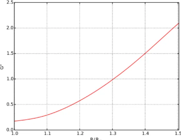
6.5 Value ofG2(R) for different value of Π⋆ . . . 106
6.6 Value of d Gd R2(R) speed on the axis for different value of Π⋆ . . . 106
6.7 Values of expansion factor F(R) for different value of Π⋆ . . . 107
6.8 Values of β(R)speed on the axis for different value of Π⋆ . . . 107
6.9 Value of GR22(R)for different values of Π⋆ . . . 108
6.10 Value of d Gd R2(R) for different values of Π⋆ . . . 108
6.11 Factorβon the axis for the list of solution S1 to S8 . . . 111
7.1 Evolution of the radial velocity along the polar axis for solutions in a Schwarzschild metric, with m1= 0( blue) andm1= −0.078(red). The second case has a smaller terminal velocity. . . 114
7.2 Field lines for a solution in a Schwarzschild metric, with parameters λ = 1.0, κ = 0.2,δ = 1.2, ν = 0.8,ℓ= 0,µ = 0.1, e1= 0 and m1= 0 (left) and m1= −0.078 (right). We note that the case m1= −0.078 corresponds to a more tightly collimated jet. Lengths are in units of the Schwarzschild radius. The red lines are connected to the magnetosphere of the central object while the green lines are connected to the disk. The separating line is in blue and the light cylinder in black. . . 115
7.3 Three-dimensional (3D) representation of the field lines and streamlines for the thermally collimated solution K1 at the base of the jet and for two flux tubes. The blue lines correspond to streamlines, the red lines to magnetic field lines. The length is in units of the Alfv´en radius, that is, ten times the Schwarzschild radius. . 117
7.4 Poloidal field lines and ”light cylinder” for the thermally collimated solution K1, for λ = 1.0, κ = 0.2, δ = 2.3, ν = 0.9, µ = 0.1,ℓ= 0.05, e1= 0. The length unit is the Schwarzschild radius. . . 117
7.5 Lorentz factor γ for theK1 (blue line) and K2 (red line) solutions. Distances are given in Schwarzschild radius units. . . 119
7.6 Poloidal field lines and ”light cylinder” for the K2 solution, that is, forλ = 1.0, κ = 0.2,δ = 1.35, ν = 0.46223, µ = 0.1,ℓ= 0.05, e1= 0. Distances are given in Schwarzschild radius units. . . 120
7.7 Plot of the longitudinal forces, that is, along the field line, for the K2 solution, along the lineα = 0.01αlim. Distances are given in Schwarzschild radius units. . . . 121
7.8 Plot of the transverse forces, that is, perpendicular to the field line, for the K2 solution, along the line α = 0.01αlim. We see that the Lorentz force is collimating and is balanced by the electric force that decollimates. Distances are given in Schwarzschild radius units. . . 122
7.9 Relative normalized contribution to the total energy of the kinetic enthalpy hγξk and the external heating distribution hγQ/c2 along the axis. . . 122
LIST OF FIGURES
7.10 Relative normalized contribution to the total energy of the kinetic enthalpy hγξk
and the external heating distributionhγQ/c2 along the streamline α = 0.05αlim . . . 123
7.11 Lorentz factor for the nonoscillating collimated solution K3. . . 124
7.12 Poloidal field lines and ”light cylinder”for the nonoscillating collimated solutionK3, that is, for λ = 1.2, κ = 0.005, δ = 2.3, ν = 0.42, µ = 0.08,ℓ= 0.024, e1= 0. Distances are given in Schwarzschild radius units. . . 124
7.13 Poloidal field lines and ”light cylinder” for the conical solution K4, that is, for λ = 0.0143, κ = 1.451, δ = 3.14, ν = 0.8, µ = 0.41,ℓ= 0.15, e1= 0. Distances are given in Schwarzschild radius units. . . 125
7.14 Lorentz factor for the conical solution K4. Distances are given in Schwarzschild radius units. . . 125
7.15 Variation of the magnetic collimation efficiency parameter ǫ vs. the black hole spin parameter aH for K1-type, K3-type, and K4-type solutions. The value of ǫ has been normalized by|ǫ(0)|when it is negative and byǫ(0) when it is positive. . . 126
7.16 Plot of the cylindrical jet radius normalized to its value at the Alfv´en surface, G, for K1-type solutions, as a function of the distance along the polar axis, for five different values of the black hole spin aH. The function G is equal to 1 at the Alfv´en distancer = 10rs. . . 127
7.17 Plot of the Lorentz factorγforK4-type solutions when the black hole spin param-eter aH varies between−0.99and0.99. . . 127
7.18 Plot of the ratio of the cylindrical radius to the spherical radius for the conical K4-type solutions with a spin parameter aH varying between −0.99 and 0.99 vs. the distance z above the equatorial plane in units of the Schwarzschild radius. . . 128
7.19 Magnetisation parameter mapσ for K1 solution . . . 132
7.20 Magnetisation parameter mapσ for K2 solution . . . 132
7.21 Magnetisation parameter mapσ for K3 solution . . . 133
7.22 Magnetisation parameter mapσ for K4 solution . . . 133
7.23 Expansion factor G2 for different values of e1 . . . 134
7.24 Opening angle factorFfor different values of e1 . . . 134
7.25 proper velocity βγon the axis for different values ofe1 . . . 134
7.26 Transversal evolution ofβfor asymptotic z value and for different values of e1 . . . 134
7.27 Values of dimensionless model temperature for K3 solution . . . 135
7.28 Values of dimensionless model temperature for K2 solution . . . 135
7.29 Evolution for the different solution of the ratio between the Compton cooling time scale and the dynamical time scale τc/τd along the axis in function of distance R/RH . . . 137
7.30 Evolution for the different solution of the ratio between the synchrotron cooling time scale and the dynamical time scaleτs/τd along the axis in function of distance R/RH . . . 137
7.31 Temperature for K3 solution on the axis . . . 138
7.32 Temperature for K2 solution on the axis . . . 138
7.33 Distribution of the two components of the enthalpy for K3 solution on the axis . . 138
7.34 Distribution of the two components of the enthalpy for K2 solution on the axis . . 138
8.1 Value of the flux tube radius functionG2 as function of the radius for the solution I1 . . . 150
8.2 Plot of the expansion factor functionhzFas a function of the radius for the solution I1 . . . 150
8.3 Plot of the Alfv´en polar Mach number M2 as a function of the radius for the solution I1 . . . 150
8.4 Plot of the polar Mach number Π as function of the radius for the solution I1 . . 150 xiii
8.5 Longitudinal Forces on a poloidal field line plotted in orange in Fig.(8.25) for the solution I1 . . . 151 8.6 Transversal Forces on a poloidal field line represented in orange in Fig.(8.25) for
solution I1 . . . 151 8.7 Plot of the perfect fluid ΦPF, the electro-magnetic ΦEM and the total flux ΦT
normalized energy fluxes by unit of magnetic flux on the black hole horizon as a function of the latitude angle θ for solution I1. All the flux are normalized by the total flux on the polar axis Φ(A)
|ΦT(0)| . . . 152
8.8 Plot of the inertial ΦM, Lense-Thirring ΦLT, electro-magnetic ΦEM and the total flux ΦTnormalized energy fluxes by unit of magnetic flux on the black hole horizon as a function of the latitude angleθ for solution I1. All the flux are normalized by the total flux on the polar axis Φ(A)
|ΦT(0)| . . . 152
8.9 Value of the flux tube radius function G2as function of the radius for the solution I2 . . . 153 8.10 Plot of the expansion factor functionhzFas a function of the radius for the solution
I2 . . . 153 8.11 Plot of the Alfv´en polar Mach number M2 as a function of the radius for the
solution I2 . . . 153 8.12 Plot of the polar Mach number Π as function of the radius for the solution I2 . . 153 8.13 Longitudinal Forces on a poloidal field line plotted in orange in Fig.(8.26) for the
solution I2 . . . 154 8.14 Transversal Forces on a poloidal field line represented in orange in Fig.(8.26) for
solution I2 . . . 154 8.15 Plot of the perfect fluid ΦPF and the electro-magnetic ΦEM and the total flux ΦT
normalized energy fluxes by unit of magnetic flux on the black hole horizon as a function of the latitude angle θ for solution I2. All the flux are normalized by the total flux on the polar axis Φ(A)
|ΦT(0)| . . . 154
8.16 Plot of the inertial ΦM, Lense-Thirring ΦLT and electro-magnetic ΦEMand the total flux ΦTnormalized energy fluxes by unit of magnetic flux on the black hole horizon as a function of the latitude angleθ for solution I2. All the flux are normalized by the total flux on the polar axis Φ(A)
|ΦT(0)| . . . 154
8.17 Value of the flux tube radius functionG2as function of the radius for the solution I3 . . . 155 8.18 Plot of the expansion factor functionhzFas a function of the radius for the solution
I3 . . . 155 8.19 Plot of the Alfv´en polar Mach number M2 as a function of the radius for the
solution I3 . . . 156 8.20 Plot of the polar Mach number Π as function of the radius for the solution I3 . . 156 8.21 Longitudinal Forces on a poloidal field line plotted in orange in Fig.(8.27) for the
solution I3 . . . 156 8.22 Transversal Forces on a poloidal field line represented in orange in Fig.(8.27) for
solution I3 . . . 156 8.23 Plot of the perfect fluid ΦPF and the electro-magnetic ΦEM and the total flux ΦT
normalized energy fluxes by unit of magnetic flux on the black hole horizon as a function of the latitude angle θ for solution I3. All the flux are normalized by the total flux on the polar axis Φ(A)
|ΦT(0)| . . . 157
8.24 Plot of the inertial ΦM, Lense-Thirring ΦLT and electro-magnetic ΦEMand the total flux ΦTnormalized energy fluxes by unit of magnetic flux on the black hole horizon as a function of the latitude angleθ for solution I3. All the flux are normalized by the total flux on the polar axis Φ(A)
LIST OF FIGURES
8.25 Geometry of poloidal field line of solution I1 . . . 157 8.26 Geometry of poloidal field line of solution I2 . . . 157 8.27 Geometry of poloidal field line of solution I3 . . . 157 8.28 Sketch representing the current intensity isocontourIin the layer of ∆r thickness.
Blue lines are iso contour ofI. Red lines represent the boundary of the thin layer. The dotted red line is the surface of stagnation. . . 160 8.29 Celerity on the axis γβfor the M1 matched solution in green the inflow part and
in red the outflow part . . . 162 8.30 Celerity on the axis γβfor the M2 matched solution in green the inflow part and
in red the outflow part . . . 162 8.31 Celerity on the axis γβfor the M3 matched solution in green the inflow part and
in red the outflow part . . . 162 8.32 Geometry of the poloidal field lines for the M1 matched solution, in orange the
external light-cylinder, in red the stagnation radius, in green the slow-magnetosonic surface. . . 163 8.33 Geometry of poloidal field lines for the M1 matched solution, in brown the internal
light cylinder, in magenta the ergosphere. . . 163 8.34 Geometry of the poloidal field lines for the M2 matched solution, in orange the
external light-cylinder, in red the stagnation radius, in green the slow-magnetosonic surface. . . 164 8.35 Geometry of poloidal field lines for the M2 matched solution, in brown the internal
light cylinder, in magenta the ergosphere. . . 164 8.36 Geometry of the poloidal field lines for the M3 matched solution, in orange the
external light-cylinder, in red the stagnation radius, in green the slow-magnetosonic surface. . . 164 8.37 Geometry of poloidal field lines for the M3 matched solution, in brown the internal
light cylinder, in magenta the ergosphere. . . 164 8.38 Mass flux by unit of solid angle absorbed by the black hole for the matching
solution M1 . . . 166 8.39 Normalized material apparition rate by unit of solid angle for the matching solution
M1 . . . 166 8.40 Noether energy and angular momentum flux by unit of solid angle absorbed by the
black hole for the matching solution M1 . . . 166 8.41 Noether energy and angular momentum flux from loading terms by unit of solid
angle for the matching solution M1 . . . 166 8.42 Mass flux by unit of solid angles absorbed by the black hole for the matching
solution M2 . . . 167 8.43 Normalized material apparition rate by unit of solid angles for the matching solution
M2 . . . 167 8.44 Noether energy and angular momentum flux by unit of solid angles absorbed by
the black hole for the matching solution M2 . . . 167 8.45 Noether energy and angular momentum flux from loading terms by unit of solid
angles for the matching solution M2 . . . 167 8.46 Mass flux by unit of solid angles absorbed by the black hole for the matching
solution M3 . . . 168 8.47 Normalized material apparition rate by unit of solid angles for the matching solution
M3 . . . 168 8.48 Noether energy and angular momentum flux by unit of solid angles absorbed by
the black hole for the matching solution M3 . . . 168 8.49 Noether energy and angular momentum flux from loading terms by unit of solid
angles for the matching solution M3 . . . 168 8.50 Surface density and current of charge for M1 solution . . . 169 xv
8.51 Surface density and current of charge for M2 solution . . . 169 8.52 Surface density and current of charge for M3 solution . . . 169 A.1 The construction of Lie derivation of a vector field (Credits : Gourgoulhon [2007]) 180
List of Tables
1.1 Table of measures of a for some Active Galaxy Nuclei (AGN) given by (Credits :
Bambi[2018]). References for each source are presented in the mentioned paper. . 2
6.1 Set of parameters for 8 solutions calculated in order to get different values of stationary radius. We keep constant the final Lorentz factor, isorotation and spin of the black hole. . . 110
7.1 Set of parameters used for the four selected solutions in the Kerr metric. K1is the solution displayed in Figs. 7.3, 7.4, and 7.5 (blue line). SolutionK2is displayed in Figs. 7.5 (red line) and 7.6, while solutionK3 is displayed in Figs. 7.11 and 7.12. Finally, solutionK4is shown in Figs. 7.13 and 7.14. . . 116
7.2 Output parameters for the four solutions in the Kerr metric. Those parameters result from the integration of the equations. . . 116
7.3 Set of parameters for a solution calculated in order to study the impact of param-etere1 around this solution . . . 133
8.1 Parameter values (with10−3 accuracy) for solution I1 . . . 149
8.2 Parmameter values (with10−3 accuracy) for solution I2 . . . 152
8.3 Parmameter values (with10−3 accuracy) for solution I3 . . . 155
8.4 Set of parameter of matched outflow solution . . . 162
8.5 Values for minimal conditions of matching function for each inflow solution . . . . 162
8.6 Value of the dimensionnless parameters for a black hole ofMH = 6, 6 ×10⁹M⊙ and B⋆,out= 1G . . . 165
List of symbol
Physical Constant
G = 6, 674× 10−8cm3.g−1.s−2 Gravitational constant
c = 2, 997 × 1010cm.s−1 Speed of light in vacuum
kB= 1,380 × 10−16g.cm2.s−2.K−1 Boltzmann constant
σT= 6.65 × 1025cm2 Thomson cross section
Geometry of space time and foliation
M Spacetime g Spacetime metrics onM TP(M ) Tangent space to M onP ∇ Covariant derivative on (M , g) Γσ µν Christoffel symbols Σ Space manifold ⊂ M n Normal to Σ γ Spatial metrics on Σ p Orthogonal projector on Σ D Covariant derivative on (Σ,γ)
K Second fondamental form
h Lapse function
hr, hθ, hφ=̟ Line element for Kerr metrics
β Shift of coordinate vector
ω Shift of coordinate pulsation
a Fiducial observer acceleration
η Stationarity Killing vector
ξ Axi-symetry Killing vector
H Horizon null hypersurface
ei Natural basis of T (Σ)
ǫi Orthonormal basis of T (Σ)
Ω Four speed hyperboloid manifold ⊂ T (M )
C+ Future light cone ⊂ T (M ) µ space phase of particles
ǫ Volum form on M ω Volum form on Ω orC+ µ Volume form of space phase
Physical quantity
J Angular momentum of the Black-Hole
MH Angular momentum of the Black-Hole
rs Schwarzschild radius
a Rotation of black hole parameter
u Generic four speed
f , f+, f−, fr, fγ Distribution function of particles
I+,I−, Ir Collision integrals or scattering operator
T, Tfl, Tr mEM Energy momentum tensor, for fluid, electromagnetic field
kN, km Number, mass Injection rate per unit of volume in fluid reference frame
k Force due to collision between fluid species
F Electro-magnetic tensor
E Electric field measured by fiducial observer Ω Isorotation function
B Magnetic field measured by fiducial observer
A Magnetic flux
j Electric four-currant
I Electric intensity
ρe Electric density measured by fiducial observer
J Electric currant measured by fiducial observer
s Entropy flux density
T Temperature
ξc2 Specific enthalpy
e Internal energy
ρ0 mass density un the fluid reference frame
V Fluid velocity measured by fiducial observer
γ Lorentz factor
ΨA Mass flux par unit of magnetic flux
L Total specific angular momentum
E Total specific energy
MAlf Alfv´en Mach number
σ Magnetization parameter
Model quantity
P⋆ Intersection between axis an Alfv´en surface
r⋆ Radius of Alfv´en surface ⋆ Evaluation onP⋆
M2 Alfv´en Mach number on the axis
G2 Dimensionless cylindrical radius
F Expansion factor
Π Dimensionless axis pressure
R Dimensionless radius
λ Dimensionless rate of angular momentum flux per unit of magnetic flux
κ Deviation from pressure sphericity
δ Logarithmic derivation of Ψ2
A on polar axis
ν Ratio between escape velocity andV⋆
l Dimensionless withr⋆ spin of the black hole
µ Dimensionless Schwarzschild radius
e1 Logarithmic variation of energy
LIST OF TABLES
Astrophysical units and quantity
M⊙= 1, 988 × 1033g Solar mass
Tb= 5 × 10¹⁰− 5 × 10¹²K Brightness temperature of M87 source
L = 2, 7 × 1042erg.s?1 Bolometric luminosity of M87 source
B10rs= 1 − 15G Magnetic field at10rs for M87 source
MH = (6, 6 ± 0.4) × 109M⊙ Mass of supermassive black hole of M87
Chapter 1
Introduction
Contents
1.1 References . . . . 5
Extra-galactic jets are astrophysical phenomena of collimated magnetized relativistic plasma outflows traveling through space in the two opposite directions. The bipolar outflows are always associated to accretion disks. The accretion around a central super-massive black hole seems to be the cause of the launching of relativistic jets. These jets are also present in accreting X-ray binary systems, Gamma Ray Bursts (GRBs) and micro-quasars. Many types of high en-ergy astrophysical sources can be explored in order to explain the jet formation and evolution, the mechanisms of acceleration and collimation of plasma outflows and the power involved in them. Indeed, these powerful phenomena involve high energy particles physics, fluid mechanics, magnetohydrodynamics, turbulence and shocks in flows, non-equilibrium thermodynamics, gen-eral relativity, and numerical simulation,... In short, they are still relatively poorly understood phenomena and are a very active field of current astrophysical researches.
In this introduction, we do not pretend to make a complete state of the art regarding obser-vations of extragalactic jets and accretion disks around black holes. Thus, we present a summary of observations that give some jet properties and an order of magnitude of the quantities we need to model the jet launching and propagation into the inter-galactic medium. Here we restrict our presentation to jets in blazars and radiosources. Our model has application to microquasars or GRB but the range of spatial, temporal and luminosity scales is different.
Object a∗ (Iron) IRAS13224-3809 > 0.99 Mrk110 > 0.99 NGC4051 > 0.99 1H0707-495 > 0.98 RBS1124 > 0.98 NGC3783 > 0.98 NGC1365 0.97+0.01−0.04 Swift J0501-3239 > 0.96 PDS456 > 0.96 Ark564 0.96+0.01−0.06 3C120 > 0.95 Mrk79 > 0.95 MCG-6-30-15 0.91+0.06−0.07 TonS180 0.91+0.02−0.09 1H0419-577 > 0.88 IRAS00521-7054 > 0.84 Mrk335 0.83+0.10−0.13 Ark120 0.81+0.10−0.18 Swift J2127+5654 0.6+0.2−0.2 Mrk841 > 0.56 Fairall9 0.52+0.19−0.15
Table 1.1 – Table of measures ofafor some Active Galaxy
Nuclei (AGN) given by (Credits : Bambi [2018]).
Refer-ences for each source are presented in the mentioned paper.
We now get some measurements of supermassive black hole spin. How-ever measurement of the spin param-eter a of supermassive black holes is currently an issue in astrophysical ob-servations. Different techniques have been explored. A technique consists in analyzing the Kα iron line. Bambi
[2013] presents the results obtained for nearby extragalactic jets (see Tab.1.1). These super-massive black holes ex-hibit spin between 0.56 (forMrk841) to quasi maximally rotating black hole (e.g. Mrk110). To derive the spin it is necessary to model the disk and the shape of the corona. This kind of technique also allows Choudhury et al. [2018] to test general relativity in strong fields, using Johansen met-ric, which deviates from Kerr metric. They apply this method to Mrk 335 and without deviation to general rela-tivity, they find a value between 0.9 et 0.97. Which is quite a high value of spin compared to the one mentioned in Tab.(1.1), (Parker et al. [2014]). An-other technique was used byGou et al.
[2014] to measure the spin of the black hole of Cygnus X-1 binary.
Nevertheless these methods are model dependent for the accretion disk. Such kind of methods and others technics are efficient for measuring black hole spin in X-ray binaries. X-ray binaries or microquasars may be less suitable for steady-state modeling because the variability of accretion has short time scales between hours and months.
Let us also mention the very important detection of gravitational waves (Abbott et al.[2016]) resulting from a fusion of two black holes, and whose pattern gives us a strong indication on the masses, spins of the initial and final black holes. However, this technique does not allow to measure the spin of black holes that do not emit or only faint gravitational waves.
It is now recognized that jets from AGN are made of several components. It seems that outflow has at least two components, a surrounding disk wind and a spine jet the source of which is subject to discussion. Indeed, the spine jet plasma may come from the accreting material or from the black hole corona. But also pairs may be created by highly energetic photons emitted from the disk.
To explain the peculiar emission of BL Lac objects,Ghisellini et al.[2005] proposed a transver-sally structured jet model with two components. This two-component transverse structure was also used by Sikora et al. [2016] to explain blazar emission. Sikora et al. [2016] develop such a stratification model for the emission of strong-line blazars. It has also be done by Gaur et al.
[2017] to study the energy distribution of non thermal particles in the blazar PKS 2155-304.
Fabian and Rees [1995]; Henri and Pelletier [1991]; Sol et al.[1989] studied theoretically the two component models. Henri and Pelletier [1991] explore the idea of a relativistic central jet composed of electron positron pairs and surrounded by classical Magneto-Hydrodynamic (MHD)
CHAPTER 1. INTRODUCTION
wind. Dynamical interactions between components are also explored. For example Gracia et al.
[2009] explain the collimation of the spine jet by the presence of an efficiently collimated outer-disk wind component. Hervet et al. [2017] show the role of shock reflection in relativistic transverse stratified jets, for formation and motion of knots.
Numerical simulations including Special Relativistic Magneto-Hydrodynamic (SRMHD) or General Relativistic Magneto-Hydrodynamic (GRMHD) have also been performed to model the jet formation and study their two components structuration. Millas et al. [2017] explored, using the AMR-VAC simulation code, the role of toroidal velocity and magnetic field in the stability of two-component jets. Many simulations after the ones ofMcKinney and Blandford [2009] ex-hibit Poynting flux force-free spine jets. From numerical simulations, McKinney et al. [2012] andTchekhovskoy et al. [2011] have also derived a scaling law from between accretion rate and magnetic flux threading the black hole horizon. In Zamaninasab et al.[2014] the authors justify this scaling law from observations and analysis.
The ejection process, in particular in the spine jet, is deeply linked to the accretion process on the central object. It is therefore essential to study the accretion on the central object to see how it can influence the jet. The standard accretion-ejection models include accretion models dominated by advection. These accretion models are applied to the internal part of the disks, except for very high accretion efficiency, (see Narayan and Yi [1994]). The study of accreting flows is also motivated by rotational energy transfer from the black hole to external medium. The Penrose process (Penrose[1969]) and the Blandford&Znajek process (Blandford and Znajek
[1977]) are suspected to play an important role regarding the power observed in jets.
Nevertheless, to evaluate them properly, it is necessary to solve the GRMHD equations up to the horizon of the black hole. These process are not fully explained. At some time a controversy debate occurred about the the ”Meissner effect”. Komissarov and McKinney [2007] took part in this debate, showing that solutions of magnetic fields are different in vacuum electro-dynamics and in MHDs. The authors conclude that the black hole horizon ”Meissner effect” does not hold for highly conductive magnetospheres. Nathanail and Contopoulos [2014] also get the same conclusion about ”Meissner effect”. They calculate solution that extract of black hole rotational energy via Poynting flux. They solve force free solutions of Graad-Shafranov equation for a Kerr magnetosphere. Their solutions are calculated for three different geometries (to infinite) and high values of black hole spin. They smoothly cross the inner and outer light cylinders.
Komissarov [2009] also discusses the difference between both processes and the interpretation of Blandford&Znajek one. The pure Penrose process, because of the small number of particle fissions in the ergosphere that satisfy the process conditions, seems almost inefficient. (Bardeen et al.[1972], Wald [1974]). However, Wagh et al. [1985] proved that the electromagnetic field may supply the required energy to push particles into negative energy orbits. This allows to obtain Penrose type extraction. The energetic interaction between the black hole rotational energy and the ideal steady-stateMHDfields have been studied byTakahashi et al.[1990] andHirotani et al.
[1992]. The coupling between the fluid field and the electromagnetic field allows an effective Penrose process. Numerical simulations also seem to show that the extraction process plays an important role in jet formation. In most of the simulations (Komissarov 2005,McKinney 2006), the extraction is dominated by the Poynting flux.
The central part of AGNs is possibly filled with high-energy photons from the disk. These pho-tons can be at the origin of a mechanism for creating pairs (electron-positron, see Rees [1984]). It can explain part of the core material of the jet. In fact, this mechanism, witch loading material on magnetic field lines, can (a) fill the environment of the black hole (b) feed an accretion into the black hole (inflow) and (c) launch a spine jet (outflow) on the same fieldline. The works of Globus and Levinson [2013] and Globus and Levinson [2014] explore the importance of this phenomena for final jet energy composition. Indeed for a magnetic field-line passing through the horizon, in this treatment the energy flux inside the jet comes from the pair energy injection and 3
energy flux extraction from the black hole.
The study of a magnetized plasma can be done using a microscopic description (Boltzmann’s equation, Vlasov’s equation...) or a mesoscopic description - MHD - which can be derived from the microscopic description. The MHD description will be favored in this work. The microphysics description will serve to us for deriving source terms due to fluid species interaction.
Research on plasma flow is done in two directions, • Numerical simulations
They allow to study the evolution over time of a given field configuration. The ambition to test more complex physical effects and situations motivate the improvement of the digital power and efficiency of algorithms.
• The resolution of steady-state MHD equations.
It has been chosen here. It consists to solve a partial differential equation system of mixed elliptic-hyperbolic type. The resolution of this system is very complex because of the singular points in the equations whose position can only be determined during the calculations. That is why we will look for a subset of solutions of these equations.
Figure 1.1 – Radio images of the galaxy M87 at different scales (Credits : Image courtesy of NRAO/AUI)
It seems reasonable to add the axi-symmetry assumption. Indeed, jets from AGN such as M87 seem relatively stable and axisymmetric on a spatial scale of few hundred parsec ( see400pc
Figs.1.1). The quantities of our problem now depend on only 2 variables x1, x2. The auto-similarity hypothese consists in choosing for the fundamental functions of the problem f (x1, x2)
CHAPTER 1. INTRODUCTION
a form of the type : f (x1, x2) = F(x1, fi =1...(x2)). Where F(x1, fi =1...) is given explicitly and the
fi(x2) are unknown real functions. If the F functions are correctly chosen then, injecting them
into the equations of the MHD allows a decoupling of the variables. Thus we obtain an ordinary numerically integrable differential system of thefi(x2)functions. In such a treatment, the variable
x1 is called the auto-similarity variable.
More concretely about the MHD, there are two main classes of self-similar models.
• Radial self-similarity : which is adapted to disk wind. For the non-relativistic flow,Li[1995] shows how to connect the wind of solutions to the disk characteristics. While Ferreira
[1997] constructs solutions for magnetically driven outflow from Keplerian disks. Vlahakis et al. [2000] build self-similar solutions that cross all critical points. Then Vlahakis and K¨onigl [2003a,b] extend these models for relativistic flows and study some of the solutions. Nevertheless the radial self-similar solution cannot by construction, applied to the polar axis. That’s one of the reasons this kind of solutions is well adapted for disk-winds.
• Meridional self similar solution : this type is most adapted to describe flows close to the rotational axis. Tsinganos and Trussoni [1991] began to build the meridional self-similar model for MHD flows. Then Sauty and Tsinganos [1994] exposed two classes of solutions and a criterion which allows to characterize these flows. ThenMeliani et al.[2006] extended a meridional self-similar model for magnetized flow around Schwarzschild black hole. And
Globus et al. [2014] extended it to the magnetized flows around Kerr black hole.
The purpose of this work is to construct solutions from the accretion on the horizon of the black hole and the collimated ejection up to infinity. This allows us to ask ourself the question of acceleration and collimation of the spine jet. We want to explore the amount of energy in the jet coming from the rotational energy of the black hole and the amount coming from the loading term (pairs creation mechanism).
In order to build these solutions, we will start with a presentation of the theoretical foundations of the model. First of all, we will present properties of the 3+1 formalism in Ch.(2). Then we will derive in Ch.(3) the equations of the MHD for a magnetized fluid filled by the pair creation mechanism from statistical physics in curved space-time. Finally, we will derive the main results concerning the General Relativistic Axi-symmetric Stationary Ideal Magneto-Hydrodynamic (GRASIMHD) with source terms. The source terms are necessary to build complete solutions outside the hypothesis of a rarefied flow and are presented in Ch.(4).
The way to find solutions for the considered equations will be done using an extension of the meridionnal self-similar model in Kerr metric built by Globus et al. [2014]. We present the construction of this model in Ch.(5). Then we develop the numerical method used to solve the equations of the models in Ch.(6).
In the Ch.(7), we will present the main characteristics of the ouflow solutions generated by our model. These solutions could be used to describe the flow of magnetized plasma from the spine jets. Finally we in Ch.(8) we explore the use of this meridional self-similar model to build inflow solutions, allowing us to model a magnetized accretion onto the black hole. We have also to quantified the energy exchanges between the rotating black hole and the MHD fields. The articulation of these two types of flow allows us to build complete solutions using source terms. We have to estimate the source term values.
1.1
References
B. P. Abbott, R. Abbott, T. D. Abbott, M. R. Abernathy, and & co Acernese. Observation of gravitational waves from a binary black hole merger. Phys. Rev. Lett., 116:061102, Feb 2016. doi: 10.1103/PhysRevLett.116.061102. URL https://link.aps.org/doi/10.1103/
PhysRevLett.116.061102. 2
C. Bambi. Measuring the Kerr spin parameter of a non-Kerr compact object with the continuum-fitting and the iron line methods. jcap, 8:055, August 2013. doi: 10.1088/1475-7516/2013/08/ 055. 2
Cosimo Bambi. Astrophysical black holes: A compact pedagogical review. Annalen der Physik, 530(6):1700430, 2018. doi: 10.1002/andp.201700430. URLhttps://onlinelibrary.wiley.
com/doi/abs/10.1002/andp.201700430. xvii, 2
J. M. Bardeen, W. H. Press, and S. A. Teukolsky. Rotating Black Holes: Locally Nonrotating Frames, Energy Extraction, and Scalar Synchrotron Radiation. apj, 178:347–370, December 1972. doi: 10.1086/151796. 3
R. D. Blandford and R. L. Znajek. Electromagnetic extraction of energy from Kerr black holes.
mnras, 179:433–456, May 1977. doi: 10.1093/mnras/179.3.433. 3
K. Choudhury, S. Nampalliwar, A. B. Abdikamalov, D. Ayzenberg, C. Bambi, T. Dauser, and J. A. Garcia. Testing the Kerr metric with X-ray Reflection Spectroscopy of Mrk 335 Suzaku data. ArXiv e-prints, September 2018. 2
A. C. Fabian and M. J. Rees. The accretion luminosity of a massive black hole in an elliptical galaxy. mnras, 277:L55–L58, November 1995. doi: 10.1093/mnras/277.1.L55. 2
J. Ferreira. Magnetically-driven jets from Keplerian accretion discs. aap, 319:340–359, March 1997. 5
Haritma Gaur, Liang Chen, R. Misra, S. Sahayanathan, M. F. Gu, P. Kushwaha, and G. C. Dewangan. The hard x-ray emission of the blazar pks 2155?304. The Astrophysical Journal, 850(2):209, 2017. URLhttp://stacks.iop.org/0004-637X/850/i=2/a=209. 2
G. Ghisellini, F. Tavecchio, and M. Chiaberge. Structured jets in TeV BL Lac objects and ra-diogalaxies. Implications for the observed properties. aap, 432:401–410, March 2005. doi:
10.1051/0004-6361:20041404. 2
N. Globus and A. Levinson. Loaded magnetohydrodynamic flows in Kerr spacetime. prd, 88(8): 084046, October 2013. doi: 10.1103/PhysRevD.88.084046. 3
N. Globus and A. Levinson. Jet Formation in GRBs: A Semi-analytic Model of MHD Flow in Kerr Geometry with Realistic Plasma Injection. apj, 796:26, November 2014. doi: 10.1088/
0004-637X/796/1/26. 3
N. Globus, C. Sauty, V. Cayatte, and L. M. Celnikier. Magnetic collimation of meridional-self-similar general relativistic MHD flows.prd, 89(12):124015, June 2014. doi: 10.1103/PhysRevD.
89.124015. 5
L. Gou, J. E. McClintock, R. A. Remillard, J. F. Steiner, M. J. Reid, J. A. Orosz, R. Narayan, M. Hanke, and J. Garc´ıa. Confirmation via the Continuum-fitting Method that the Spin of the Black Hole in Cygnus X-1 Is Extreme. apj, 790:29, July 2014. doi: 10.1088/0004-637X/790/1/ 29. 2
J. Gracia, N. Vlahakis, I. Agudo, K. Tsinganos, and S. V. Bogovalov. Synthetic Synchrotron Emission Maps from MHD Models for the Jet of M87. apj, 695:503–510, April 2009. doi:
10.1088/0004-637X/695/1/503. 3
G. Henri and G. Pelletier. Relativistic electron-positron beam formation in the framework of the two-flow model for active galactic nuclei. apjl, 383:L7–L10, December 1991. doi: 10.1086/
CHAPTER 1. INTRODUCTION
O. Hervet, Z. Meliani, A. Zech, C. Boisson, V. Cayatte, C. Sauty, and H. Sol. Shocks in relativistic transverse stratified jets. A new paradigm for radio-loud AGN. aap, 606:A103, October 2017.
doi: 10.1051/0004-6361/201730745. 3
K. Hirotani, M. Takahashi, S.-Y. Nitta, and A. Tomimatsu. Accretion in a Kerr black hole magnetosphere - Energy and angular momentum transport between the magnetic field and the matter. apj, 386:455–463, February 1992. doi: 10.1086/171031. 3
S. S. Komissarov. Observations of the Blandford-Znajek process and the magnetohydrodynamic Penrose process in computer simulations of black hole magnetospheres. mnras, 359:801–808, May 2005. doi: 10.1111/j.1365-2966.2005.08974.x. 3
S. S. Komissarov. Blandford-Znajek Mechanism versus Penrose Process. Journal of Korean
Physical Society, 54:2503, June 2009. doi: 10.3938/jkps.54.2503. 3
S. S. Komissarov and J. C. McKinney. The ‘Meissner effect’ and the Blandford-Znajek mechanism in conductive black hole magnetospheres. mnras, 377:L49–L53, May 2007. doi: 10.1111/j.
1745-3933.2007.00301.x. 3
Z.-Y. Li. Magnetohydrodynamic disk-wind connection: Self-similar solutions. apj, 444:848–860, May 1995. doi: 10.1086/175657. 5
J. C. McKinney. General relativistic magnetohydrodynamic simulations of the jet formation and large-scale propagation from black hole accretion systems. mnras, 368:1561–1582, June 2006.
doi: 10.1111/j.1365-2966.2006.10256.x. 3
Jonathan C. McKinney and Roger D. Blandford. Stability of relativistic jets from rotating, ac-creting black holes via fully three-dimensional magnetohydrodynamic simulations. mnras, 394: L126–L130, March 2009. doi: 10.1111/j.1745-3933.2009.00625.x. 3
Jonathan C. McKinney, Alexander Tchekhovskoy, and Roger D. Blandford. General relativistic magnetohydrodynamic simulations of magnetically choked accretion flows around black holes.
Monthly Notices of the Royal Astronomical Society, 423(4):3083–3117, 2012. doi: 10.1111/j.
1365-2966.2012.21074.x. URLhttp://dx.doi.org/10.1111/j.1365-2966.2012.21074.x.
3
Z. Meliani, C. Sauty, N. Vlahakis, K. Tsinganos, and E. Trussoni. Nonradial and nonpolytropic astrophysical outflows. VIII. A GRMHD generalization for relativistic jets. aap, 447:797–812, March 2006. doi: 10.1051/0004-6361:20053915. 5
D. Millas, R. Keppens, and Z. Meliani. Rotation and toroidal magnetic field effects on the stability of two-component jets. mnras, 470:592–605, September 2017. doi: 10.1093/mnras/stx1288. 3
Ramesh Narayan and Insu Yi. Advection-dominated Accretion: A Self-similar Solution. apj, 428: L13, June 1994. doi: 10.1086/187381. 3
A. Nathanail and I. Contopoulos. Black Hole Magnetospheres. apj, 788:186, June 2014. doi:
10.1088/0004-637X/788/2/186. 3
M. L. Parker, D. R. Wilkins, A. C. Fabian, D. Grupe, T. Dauser, G. Matt, F. A. Harrison, L. Brenneman, S. E. Boggs, F. E. Christensen, W. W. Craig, L. C. Gallo, C. J. Hailey, E. Kara, S. Komossa, A. Marinucci, J. M. Miller, G. Risaliti, D. Stern, D. J. Walton, and W. W. Zhang. The NuSTAR spectrum of Mrk 335: extreme relativistic effects within two gravitational radii of the event horizon? mnras, 443:1723–1732, September 2014. doi: 10.1093/mnras/stu1246. 2
R. Penrose. Gravitational Collapse: the Role of General Relativity. Nuovo Cimento Rivista Serie, 1, 1969. 3
M. J. Rees. Black Hole Models for Active Galactic Nuclei. araa, 22:471–506, 1984. doi: 10.1146/
annurev.aa.22.090184.002351. 3
C. Sauty and K. Tsinganos. Nonradial and nonpolytropic astrophysical outflows III. A criterion for the transition from jets to winds. aap, 287:893–926, July 1994. 5
Marek Sikora, Mieszko Rutkowski, and Mitchell C. Begelman. A spine-sheath model for strong-line blazars. mnras, 457:1352–1358, April 2016. doi: 10.1093/mnras/stw107. 2
H. Sol, G. Pelletier, and E. Asseo. Two-flow model for extragalactic radio jets. mnras, 237: 411–429, March 1989. doi: 10.1093/mnras/237.2.411. 2
M. Takahashi, S. Nitta, Y. Tatematsu, and A. Tomimatsu. Magnetohydrodynamic flows in Kerr geometry - Energy extraction from black holes. apj, 363:206–217, November 1990. doi: 10.
1086/169331. 3
Alexander Tchekhovskoy, Ramesh Narayan, and Jonathan C. McKinney. Efficient generation of jets from magnetically arrested accretion on a rapidly spinning black hole. Monthly Notices
of the Royal Astronomical Society: Letters, 418(1):L79–L83, 2011. doi: 10.1111/j.1745-3933.
2011.01147.x. URL http://dx.doi.org/10.1111/j.1745-3933.2011.01147.x. 3
K. Tsinganos and E. Trussoni. Analytical studies of collimated winds. II - Topologies of 2-D helicoidal MHD solutions. aap, 249:156–172, September 1991. 5
N. Vlahakis and A. K¨onigl. Relativistic Magnetohydrodynamics with Application to Gamma-Ray Burst Outflows. I. Theory and Semianalytic Trans-Alfv´enic Solutions. apj, 596:1080–1103, October 2003a. doi: 10.1086/378226. 5
N. Vlahakis and A. K¨onigl. Relativistic Magnetohydrodynamics with Application to Gamma-Ray Burst Outflows. II. Semianalytic Super-Alfv´enic Solutions.apj, 596:1104–1112, October 2003b.
doi: 10.1086/378227. 5
N. Vlahakis, K. Tsinganos, C. Sauty, and E. Trussoni. A disc-wind model with correct crossing of all magnetohydrodynamic critical surfaces. mnras, 318:417–428, October 2000. doi: 10.1046/
j.1365-8711.2000.03703.x. 5
S. M. Wagh, S. V. Dhurandhar, and N. Dadhich. Revival of the Penrose process for astrophysical applications. apj, 290:12–14, March 1985. doi: 10.1086/162952. 3
R. M. Wald. Energy Limits on the Penrose Process. apj, 191:231–234, July 1974. doi: 10.1086/
152959. 3
M. Zamaninasab, E. Clausen-Brown, T. Savolainen, and A. Tchekhovskoy. Dynamically important magnetic fields near accreting supermassive black holes. nat, 510:126–128, June 2014. doi:
Chapter 2
3+1 Methods
Contents
2.1 Geometry of imbedded hypersurfaces in spacetime . . . 10 2.2 Framework and notations . . . 10 2.2.1 Hypersurfaces . . . 11 2.2.2 Curvature of manifolds . . . 13 2.2.3 Link between connections . . . 15 2.3 Foliation of spacetime . . . 16 2.3.1 Lapse function . . . 16 2.3.2 Shift vector . . . 17 2.3.3 3+1 decomposition of the metric . . . 17 2.3.4 Acceleration of Fiducials Observers (FIDO) . . . 18 2.4 A foliation of Kerr spacetime . . . 18 2.4.1 Kerr metric . . . 19 2.4.2 Choice of foliation system . . . 20 2.4.3 Expression of the extrinsic curvature . . . 21 2.4.4 Spatial operators in Boyer-Lindquist coordinates . . . 21 2.5 Conclusion . . . 23 2.6 References . . . 23
The 3+1 formalism is an approach to general relativity using the notion of foliation of four di-mensional spacetime varieties (M) with three dimensional imbedded sub-varieties (Σt). These
sub-varieties must be ”similar” to space. Such that, the general spacetime induces a Riemannian metric. In others words the induced metric is a definite positive bilinear form. This formalism makes possible to systematically rewrite the equations of general relativity in a convenient form. This form is similar to the equations of classical mechanics even if it incorporates relativistic ef-fects. In this formulation the physical meaning of the equations of general relativity appears more clearly. The 3+1 decomposition of Einstein’s equations also gives a new perspective on general relativity, the so-called chrono-geometric interpretation of general relativity [Wheeler,1964], i.e. the evolution over time of the geometry of three dimensional manifold representing space.
The 3+1 formalism also allows us to introduce an observer and a particular frame in which the different physical quantities related to magneto-hydrodynamics are measured. Indeed some quantities as the electric and the magnetic fields have a meaning only in a considered reference frame. This is an important requirement to give a physical meaning to the field we study.
Historically, the development of these methods started at the beginning of last century with the work of Darmois, Lichnerowicz [1939] and Choquet-Bruhat and Geroch [1969]. These last two authors were the first to prove the unicity of the solution to Cauchy’s problem arising from the 3+1 decomposition of Einstein’s equations. After the Second World War, the 3+1 formalism received great interest because it serves as a basis to the work on Hamiltonian formulation of general relativity, the same way as the chrono-dynamic formulation in general relativity did, (see
Arnowitt et al. [2008]). Later on this formalism became one of the essential tools of numerical relativity.
This chapter is not an exhaustive treatment of the 3+1 decomposition methods. It is a sum-mary of useful results and definitions used further down for calculations. This chapter is inspired from the work done by Gourgoulhon[2007]. We shall first study the geometry of the submerged submanifold. Then we shall see how to reconstruct the geometry of full time space from the folia-tion. Finally we shall express the the Kerr’s spacetime foliation and calculate the useful remaining associated quantities.
2.1
Geometry of imbedded hypersurfaces in spacetime
Before introducing the foliation of spacetime, let us give some general results on imbedded sub-manifolds. These results are valid for any type of submanifold or spacetime, independently of the fact that the considered spacetime is a solution or not of Einstein’s equations. Moreover these results can be applied to the black hole horizon, which is a submanifold and is not directly issued from a 3+1 foliation. These results constitute the first step to establishe the tools useful for the 3+1 decomposition of the covariant equations.
2.2
Framework and notations
Let us call M a smooth spacetime manifold and g a Lorentzian metric on M with a signature
(−;+;+;+). Here we consider only time orientable spacetime manifoldM. This means that a
con-tinuous construction of future-directed and past-directed for non-spacelike vectors can be made over the entire manifold.
CHAPTER 2. 3+1 METHODS
space of M around point P. This is a 4-dimensional vectorial space. We call TP⋆(M ) its four dimensional dual space. It contains the ordinary one form. In order to simplify our notations, except in case of ambiguity, we use the same notation for the dual of the tangent space, the tensorial product of the tangent space with itself and the tangent space itself.
We adopt the following convention for the tensor indices. Greek letters run for 4 dimensions,
{0, 1, 2, 3}. We use as far as possible the first letter of the greek alphabet for uncontracted indices such asα, β, γ and other letters such as µ, νfor contracted indices. Latin letters are used for the 3 dimensions,1, 2, 3.
If(xα) is a mapping ofM then we noteeα the natural basis associated to this mapping. We also note Γαβγ the Christoffel symbols, which are associated to this system of coordinates and the covariant derivative∇.
We also note u · v = g(u,v) the scalar product, ⊕ the direct sum of the vectorial space and ⊗
the tensor product.
2.2.1 Hypersurfaces
A hypersurface ofM is a subset ofM, which is a three dimensional submanifold. Definition
The first method, the immersion method to define a hypersurface, consists in using a none zero volume part ofΣˆ ⊂ R3 to construct a parameterized subset of M. Let call it Σ⊂ M if there is a
C1-diffeomorphism Φ: ˆΣ→Σ. Then Σ is a three-dimensional imbedded manifold.
The second method is submersion. It consists by using a sufficiently smooth scalar function
t : M → R, such that we can define a three-dimensional imbedded manifold using Σ= {M ∈ M |
t (M) = 0}. This definition works only if∇t 6= 0.
We recall that the tangent space in P ∈Σis generated by all tangent vectors of allC1 curves passing throughP. Because the set ofC1 curves of Σ passing throughPis contained into the set ofC1 curves ofM, it implies that TP(Σ) ⊂ TP(M ). Note that∀dx ∈ TP(Σ). We get∇t ·dx = d t, which is null because of the definition of Σ. Thus we haveTP(Σ) ⊂ (R∇t)⊥.
Normal unit vector
Using the definition of submersion, the hypersurface Σ can be locally of 3 different types, • A spatial hypersurface if the normal is a time vector g(∇t,∇t) < 0,
• A null surface if the normal is a null vectorg(∇t,∇t) = 0
• A Lorentzian surface if the normal is a spatial vector g(∇t,∇t) > 0
In the following, we concentrate our interest on the case of spatial or null hypersurfaces. In the case of spatial or Lorentzian hypersurfaces, let us define the normal unit vectorn,
n = −p ∇t
| g(∇t,∇t) |= −hc∇t , (2.1)
which defines the direction perpendicular to the 3 dimensional hypersurfaces Σ. In the case of a null hypersurface, we call ℓ the normal vector. In this case ℓ is orthogonal and also tangent to Σ. The minus sign is chosen such that the normal vector is oriented towards the future.
CHAPTER 2. 3+1 METHODS
It implies that we can decompose all tensors in different component kinds, function of the ”size” of the considered tensor. For instance,
1. the rest mass densityρ0, which has no decomposition,
2. the four electric-currentj = −ρecn+J, withJis the ”three dimensional electric-current, more
explanations will be given on the physical meaning of this decomposition on Sec.(4.1.3). 3. the energy-impulsion tensor, which can be rewritten, T = en ⊗ n + p ⊗ n + n ⊗ p + S, where
S ∈ T (Σ)2 is its spatial component and p ∈ T (Σ)its temporal one.
To obtain the spatial part of any tensor, it is enough to project each order onTP(Σ),
(p⋆M)αβ1,...,αp 1,...,βq= p α1 ν1...p αp νpp µ1 β1...p µq βqM ν1,...,νp µ1,...,µq. (2.7) 2.2.2 Curvature of manifolds
We introduce here how to calculate the derivative on a submanifold. In order to re-write the equations, such as the continuity or the Euler equation in a form similar to the classical ones, an important step is to link four dimensional-covariant derivatives ∇ to an object, which plays the role of ordinary gradient. We show that usual ”derivatives” are composed of an internal ”derivative”, which contains the variation where the submanifold is considered by itself and an extrinsic ”derivative”, which contains the curvature of the imbedded submanifold.
Intrisic curvature
Note that Σ is also a manifold, qualified as a spatial manifold, withγas induced metric. We know that there is a unique, torsion-free connection, entirely determined by the induced metricγand its partial derivatives. We will note this connectionD. By definition Dγ = 0. This connection allows us to define the intrinsic curvature, the Σ-Riemann tensorΣR also called intrinsic curvature of
(Σ,γ). Note that ∀v ∈ T (Σ),
(DαDβ− DβDα)vγ= Σ
Rγσαβvσ. (2.8)
We can use the usual formula (Eq.A.5) of the Riemann tensor with the Christoffel symbols. However, here we need to be careful and use the Christoffel symbols associated with the induced metric. D plays the role of the ordinary 3-dimensional gradient of the non-relativistic form of the equations. Thus all the spatial usual operators are defined as functions of D (see An.B.2). The expression of this affine connection is intrinsically linked to the geometry of the ”space” submanifold.
Using the concept of foliation, we see that to reconstruct the entire knowledge on the geometry of our spacetime, it is sufficient to know the intrinsic curvature of the submanifold of the foliation and the way its submanifold is bent in spacetime.
Extrinsic curvature
The form of general relativity equations makes appear the global connection∇associated to the metric g on M. This connection contains D, the Σ affine connection associated to the metric
γand also the term coming from the variation ”along”nof any tensor on M. These terms may contain some of the components along Σ. We call it the extrinsic curvature. It is due to the projection along Σ of the variation ofn. So we define what we call the second fundamental form,
K : TP(M ) × TP(M ) → R
(u, v) 7→ −p(u) · ∇p(v)n ,
(2.9) To have a good idea about the meaning of the intrinsic and the extrinsic curvatures, it is useful to give some examples using some surface imbedded in the three dimensional flat space.