Development of an engine model for an integrated aircraft design tool

Development of an Engine Model for an Integrated Aircraft

Design Tool

by

Giulia Bissinger Pantalone

B.S., Aeronautics and Astronautics, Massachusetts Institute of Technology, 2013

Submitted to the Department of Aeronautics and Astronautics in partial fulfillment of the requirements for the degree of

Master of Science in Aeronautics and Astronautics at the

MASSACHUSETTS INSTITUTE OF TECHNOLOGY

June 2015

MASSACHUSETTS INSTITUTE

OF TECHNOLOLGY

JUN 23 2015

LIBRARIES

@

Signature redacted

_..t...

A u th o r ...* ... * ... . . .V. .. . .. . .. . . . Department of Aeronautics and Astronautics

May 21, 2015

Certified by...

Signature redacted

. . .

Professor of Aeronautics and Astronautics

Thesis Supervisor

Signature redacted

A ccepted by ...

Paulo C. Lozano Associate Professor of Aeronautics and Astronautics Chair, Graduate Program Committee

Development of an Engine Model for an Integrated Aircraft

Design Tool

by

Giulia Bissinger Pantalone

Submitted to the Department of Aeronautics and Astronautics on May 21, 2015, in partial fulfillment of the

requirements for the degree of

Master of Science in Aeronautics and Astronautics

Abstract

This thesis describes the development of a new engine weight surrogate model and High Pressure Compressor (HPC) polytropic efficiency correction for the propulsion module in the Transport Aircraft OPTtimization (TASOPT) code. The goal of this work is to improve the accuracy and applicability of TASOPT in conceptual design of advanced technology, high bypass ratio, small-core, geared and direct-drive turbofan engines. The engine weight surrogate model was built as separate engine component weight surrogate models using least squares and Gaussian Process regres-sion techniques on data data generated from NPSS/WATE++ and then combined to estimate a "bare" engine weight-including only the fan, compressor, turbine, and combustor-and a total engine weight, which also includes the nacelle, nozzle, and pylon. The new model estimates bare engine weight within 10% of published

val-ues for seven existing engines, and improves TASOPT's accuracy in predicting the geometry, weight, and performance of the Boeing 737-800. The effects of existing

TASOPT engine weight models on optimization od D8-series aircraft concepts are

also discussed. The HPC polytropic efficiency correction correlation, which reduces user-input HPC polytropic efficiency based on compressor exit corrected mass flow, was implemented based on data from Computational Fluid Dynamics (CFD). When applied to TASOPT optimization studies of three D8-series aircraft, the efficiency correction drives the optimizer to increase engine core size.

Thesis Supervisor: Karen Willcox

Acknowledgments

The work presented in this thesis would not be possible without the help of many people. First and foremost, I must thank my advisor Professor Karen Willcox for her unwavering support, guidance, and encouragement over the past two years. She always made time to meet with me, even if she was on the other side of the world, and taught me valuable professional and personal lessons that I will remember the rest of my life.

Next, I would like to thank Professor Mark Drela, not only for the privilege of working with him on TASOPT, but also for the many lessons in aerodynamics and programming he has taught me over the years. I would also like to thank Elena De la Rosa Blanco for her guidance on this project, and Sergio Amaral for his help getting me up to speed on TASOPT.

The Aero/Astro department has been a defining feature of my time at MIT, and I would not be where I am today were it not for this community. To the members of the ACDL: thank you for making this lab an inspiring and friendly place to work, and for the endless enlightening conversations. In particular, I would like to thank Eric Dow and R6mi Lam, my unofficial mentors, who were always there to provide help and advice (and jokes) when I needed it. To Nina Siu, Michael Lieu, and Harriet Li: I cannot imagine the last five years of Course 16 without you guys. I also want to thank the members of DogeCube, Carlee Wagner, Philippe Kirschen, and Hugh Carson, for the memes and the laughs.

Last, but not least, I must thank my parents for their love and support through the highs and lows of my six years at MIT.

This work was funded by the US Federal Aviation Administration, Office of Envi-ronment and Energy, under FAA Award No. 09-C-NE-MIT, Amendment Nos. 028, 033, and 038, and FAA Award No. 13-C-AJFE-MIT, Amendment Nos. 006 and 011. The projects were managed by Rhett Jefferies, James Skalecky, and Joseph DiPardo

of FAA.

Any opinions, findings, and conclusions or recommendations expressed in this 5

material are those of the authors and do not necessarily reflect the views of the FAA. This work was supported in part by the NASA LEARN program, grant number NNX14AC73A.

Contents

1 Introduction 15

1.1 M otivation . . . . 15

1.2 TASOPT Background ... 16

1.3 Engine Modeling State of the Art . . . . 18

1.4 Objectives . . . ... 19

1.5 Thesis Outline . . . . 19

2 Gaussian Process Regression 21 2.1 Overview of the Method . . . . 21

2.2 Inference under GP assumption . . . . 22

2.3 Covariance Kernel . . . . 24

2.4 Choosing Hyper-parameters . . . . 25

3 TASOPT Engine Weight Model Development 27 3.1 Current M odel . . . . 27

3.1.1 WATE++ Model Assumptions . . . . 28

3.1.2 Advanced Materials Weight Reduction Methodology . . . . 31

3.2 Engine Breakdown . . . . 31

3.3 Sensitivity Analysis . . . . 34

3.4 Surrogate Models . . . . 40

3.4.1 M odel Types . . . . 40

3.4.2 Cross-Validation . . . . 40

3.4.4 Direct-Drive Turbofan, Advanced Materials 3.4.5 Geared Turbofan, Current Materials . . . . 3.4.6 Geared Turbofan, Advanced Materials . . . 4 HPC Polytropic Efficiency Correction

4.1 Background . . . . 4.2 Correction Implementation in TASOPT . . . . 5 Engine Model Validation

5.1 Engine Weight Model . . . . 5.1.1 Comparison to Published Data . . . . 5.1.2 Integrated Model Performance . . . . 5.2 HPC Efficiency Correction . . . . 5.2.1 Problem Setup . . . . 5.2.2 D 8.1 . . . . 5.2.3 D 8.2 . . . . 5.2.4 D 8.5 . . . . 6 Conclusions 6.1 Summary . . . . 6.2 Future Work . . . . A Surrogate Model Equations

A.1 Direct-Drive, Current Technology . . . . A.2 Direct-Drive, Advanced Technology . . . . A.3 Geared, Current Technology . . . . A.4 Geared, Advanced Technology . . . . B List of Boeing 737-800 Design Parameters

References . . . . 46 . . . . 50 . . . . 53 57 57 59 63 . . . . 63 . . . . 63 . . . . 65 . . . . 77 . . . . 78 . . . . 78 . . . . 8 1 ... ... 82 87 87 88 91 91 93 94 95 97 101

List of Figures

1-1 Engine station numbers, total-pressure ratios, mass flows, and spool sp eed s . . . . 18 3-1 Compressor aspect ratio variations with span . . . . 30 3-2 Turbine aspect ratio variations with span . . . . 31 3-3 Block diagram of uncertainty propagation through NPSS/WATE++. 35 3-4 GSA results for direct drive turbofan with current technology . . . . 36 3-5 GSA results for direct drive turbofan with advanced technology . . . 37 3-6 GSA results for geared turbofan with current technology . . . . 38 3-7 GSA results for geared turbofan with advanced technology . . . . 39 3-8 LS model of fan weight DOE samples (direct drive, current technology) 43 3-9 LS model of combustor weight from DOE samples (direct drive, current

technology) . . . . 44 3-10 LS model of nozzle weight from DOE samples (direct drive, current

technology) . . . . 44 3-11 LS model of nacelle weight from DOE samples (direct drive, current

technology) . . . . 45 3-12 GP model of core weight from DOE samples (direct drive, current

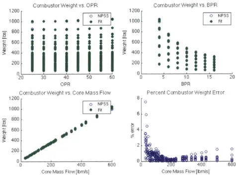
technology). The six surfaces are levels of constant inlet mass flow from 500 lbm/s to 3000 ibm/s. The color corresponds to weight, with blue being the lowest weight and red the highest. . . . . 45 3-13 Scatter plots of nozzle weight error (direct drive, current technology) 46 3-14 LS model of fan weight DOE samples (direct drive, advanced technology) 47

3-15 LS model of combustor weight from DOE samples (direct drive, ad-vanced technology) . . . . 48 3-16 LS model of nozzle weight from DOE samples (direct drive, advanced

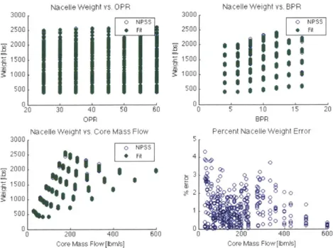
technology) . . . . 48 3-17 LS model of nacelle weight from DOE samples (direct drive, advanced

technology) . . . . 49 3-18 Scatter plots of nozzle weight error (direct drive, advanced technology) 49 3-19 LS model of fan weight DOE samples (geared, current technology) . . 51

3-20 LS model of combustor weight from DOE samples (geared, current technology) . . . . 51 3-21 LS model of nacelle weight from DOE samples (geared, current

tech-nology) . . . . 52 3-22 Scatter plots of nozzle weight error (geared, current technology) . . . 52 3-23 Scatter plots of nacelle weight error (geared, current technology) . . . 53 3-24 LS model of fan weight DOE samples (geared, advanced technology) 54 3-25 LS model of combustor weight from DOE samples (geared, advanced

technology) . . . . 55 3-26 LS model of nacelle weight from DOE samples (geared, advanced

tech-nology) . . . . 55 3-27 Scatter plots of nozzle weight error (geared, advanced technology) . . 56

3-28 Scatter plots of nacelle weight error (geared, advanced technology) . . 56 4-1 HPC efficiency versus core size for Case A . . . . 58 4-2 HPC efficiency versus core size for Case B . . . . 58 4-3 The HPC efficiency correction correlation curves for Case A for the

Shaft-Limited and Pure Scale configurations were fit to data points taken from FIGURE 4-1. . . . . 61 4-4 The HPC efficiency correction correlation curves for Case B for the

Shaft-Limited and Pure Scale configurations were fit to data points taken from FIGURE 4-2. . . . . 62

5-1 Dimensional comparison of WATE++ model and current-technology correlations to published bare engine weights. . . . . 64 5-2 Comparison of WATE++ model and current-technology correlations

as a percentage of published bare engine weight. . . . . 65 5-3 Comparison of weight model effect on fuel burn during cruise for 737-800. 69 5-4 Comparison of weight model effect on airframe geometry for D8.1. . . 71 5-5 Comparison of weight model effect on fuel burn during cruise for D8.1. 72 5-6 Comparison of weight model effect on airframe geometry for D8.2. . . 74 5-7 Comparison of weight model effect on fuel burn during cruise for D8.2. 74 5-8 Comparison of weight model effect on airframe geometry for D8.5. . . 75 5-9 Comparison of weight model effect on fuel burn during cruise for D8.5. 77 5-10 Comparison of HPC efficiency correction effect on airframe geometry

for D 8.1. . . . . 80 5-11 Comparison of HPC efficiency correction effect on fuel burn during

cruise for D 8.1. . . . . 80 5-12 Comparison of HPC efficiency correction effect on airframe geometry

for D 8.2. . . . . 83 5-13 Comparison of HPC efficiency correction effect on fuel burn during

cruise for D 8.2. . . . . 83 5-14 Comparison of HPC efficiency correction effect on airframe geometry

for D 8.5. . . . . 85 5-15 Comparison of HPC efficiency correction effect on fuel burn during

cruise for D 8.5. . . . . 86

List of Tables

3.1 Calibration Parameters . . . .

3.2 Technologies for Weight Reduction . . . . 3.3 Design Variable Ranges for WATE++ Simulations . . . 3.4 Component Percentage of Total Engine Weight . . . . 3.5 Direct-drive Component Weight Distribution Variances 3.6 Geared Component Weight Distribution Variances . . . 3.7 Direct Drive Current Technology Surrogate Models . . 3.8 Direct-drive Current Tech. Absolute Model Errors . . . 3.9 Direct Drive Advanced Technology Surrogate Models 3.10 Direct-drive Advanced Tech. Absolute Model Errors 3.11 Geared Current Technology Surrogate Models . . . . . 3.12 Geared Current Tech. Absolute Model Errors . . . . . 3.13 Geared Advanced Technology Surrogate Models . . . . 3.14 Geared Advanced Tech. Absolute Model Errors . . . . 4.1 Calibration Parameters . . . .

5.1 _{737-800 Performance Metrics: "MD" refers to Drela's weight model,} "NF basic" and "NF adv." refer to Fitzgerald's current and advanced technology correlations respectively, and "New basic" and "New adv." refer to the current and advanced technology correlations developed in C hapter 3. . . . . . . . . 30 . . . . 32 . . . . 33 . . . . 34 . . . . 40 . . . . 40 . . . . 42 . . . . 42 . . . . 47 . . . . 47 . . . . 50 . . . . 50 . . . . 53 . . . . 53 . . . . 60 68

5.2 D8.1 Performance Metrics: "MD" refers to Drela's weight model, "NF basic" and "NF adv." refer to Fitzgerald's current and advanced tech-nology correlations respectively, and "New basic" and "New adv." re-fer to the current and advanced technology correlations developed in

C hapter 3. . . . . 70

5.3 D8.2 Performance Metrics: "MD" refers to Drela's weight model, "NF basic" and "NF adv." refer to Fitzgerald's current and advanced tech-nology correlations respectively, and "New basic" and "New adv." re-fer to the current and advanced technology correlations developed in C hapter 3. . . . . 73

5.4 D8.5 Performance Metrics: "MD" refers to Drela's weight model, "NF basic" and "NF adv." refer to Fitzgerald's current and advanced tech-nology correlations respectively, and "New basic" and "New adv." re-fer to the current and advanced technology correlations developed in C hapter 3. . . . . 76

5.5 D8.1 Performance Metrics . . . . 79

5.6 D8.2 Performance Metrics . . . . 82

5.7 D8.5 Performance Metrics . . . . 84

B. 1 737-800 Airframe Parameters for TASOPT Input File . . . . 99

Chapter 1

Introduction

1.1

Motivation

Conceptual aircraft design has evolved significantly over the past 30 years to take advantage of computational methods for evaluating potential designs. The work of Torrenbeek[1], Roskam[2], and Raymer[3] all rely on historical weight and engine performance correlations, as well as empirical drag build-ups. The ACSYNT[4][5] computer-aided design tool is also largely based on historical and empirical mod-els, but uses a more detailed structural weight estimation extension, PDCYL[6]. These approaches were later extended by Knapp[7], Kroo's PASS program[8], and Wakayama's WINGMOD program[9][10] to couple the simple drag and performance models with optimization techniques, allowing for investigation of tradeoffs in a more-detailed geometry parameter space. Historical and empirical models are only valid in regions of the design space where data is available and can give overly-optimistic per-formance predictions if extrapolated inappropriately. When evaluating designs that are radically different from current technology, physics-based models provide more confidence that the optimal design is realizable.

Technological advancements such as extremely high bypass turbofan engines and advanced composite materials are outside the realm of historical data and must be modeled using fundamental physics. Additionally, the possibility of more-stringent noise and emissions policies and more-lenient operational restrictions-such as the

Free-Flight air traffic control concept-requires that the airline operations problem and the aircraft design problem be examined in conjunction. That is, designing the aircraft as a member of a fleet that can fly a variety of missions efficiently, rather than just one mission optimally.

TASOPT, by Drela[1 1], is a tool for conceptual design of transport aircraft systems that relies almost exclusively on fundamental physics to model aircraft aerodynamics, structure, and propulsion and is capable of modeling the fleet operations problem. The focus of this work is on improving the fidelity and applicability of the propulsion

model in TASOPT.

1.2

TASOPT Background

TASOPT was developed for NASA's N+3 program to maximize transport efficiency by examining aircraft, engine, and fleet operation system designs, taking advantange of new technologies and a wider variety of configurations. It uses low-fidelity physics-based models to accurately estimate weight, aerodynamic, and engine performance without the long computation time of higher-fidelity models. Historical correlations are only used in predicting engine weight and secondary structural weight. The drawback to using low-fidelity models is that TASOPT is restricted to tube-and-wing aircraft.

There are two modes in which TASOPT can run: sizing mode and optimization mode. In sizing mode, TASOPT sizes the aircraft for a particular mission, i.e. range and payload. Similarly, in optimization mode, the aircraft is sized for a particular range and payload, but quantities such as cruise altitude, cruise lift coefficient, aspect ratio, wing sweep, engine fan pressure ratio, and engine bypass ratio (among others) are varied to minimize fuel consumption. Both modes can be run for a single mission or multiple missions. In multiple mission sizing mode, the first mission is used to size the aircraft which is then flown over the subsequent missions, evaluating the off-design performance. Optimization mode for multiple missions uses as its objective function the Payload Fuel Efficiency Index, or PFEI, which is the fuel energy consumption per

payload-range. PFEI is calculated by weight-summing the fuel consumption of each mission specified. Thus, PFEI can be though of as a fleet-wide fuel consumption. TASOPT's capabilities alow the user to perform a variety of tasks, including

" modeling an existing aircraft, evaluating its off-design performance, and per-forming sensitivity studies of various design design parameters,

" analyzing the effects of advanced materials or engine technology on an airframe design,

" analyzing a strut-braced wing design or a geared or tail-mounted engine design, and

" designing an entirely new aircraft for a set of missions.

The propulsion model in TASOPT is a component-based thermodynamic cycle analysis as described by Kerrebrock[12] with variable specific heat based on a de-tailed gas-constituent model. Turbine cooling flow, which strongly influences optimal engine parameters, is also modeled and optimized for the takeoff case. On-design mode sizes the engine for cruise given a specified thrust Feng, combustor exit tem-perature TM, design fan pressure ratio FPRD, design overall pressure ratio OPRD, design bypass ratio BPRD, inlet kinetic energy defect Ki, and the flight conditions. The output of sizing mode is the engine geometry (flow-path areas), corrected spool speeds, corrected mass flows, and cooling mass flow. In off-design mode, the per-formance of the engine during takeoff, climb, and descent is evaluated for either a specified thrust or a specified combustor exit temperature based on the engine geom-etry and spool speeds computed from an assumed fan or compressor map. FIGURE 1-1 provides a sketch of the component-based engine model in TASOPT.

Since the engine is modeled only at the component level and details such as the stage count and blade geometry in each of the components is unknown, the weight of the engine cannot be calculated through a build-up of the individual part weights. However, engine component weights scale well with OPR, BPR, and mass flow, so the

RdC 74lh g 8 2. 7 4.

1.81 2 ~ 3 a 4.

g 1 .9 5 6

NI G N Nb

Figure 1-1: Engine station numbers, total-pressure ratios, mass flows, and spool speeds [11].

engine weight model in TASOPT is a correlation of these variables based on historical data.

1.3

Engine Modeling State of the Art

There exist several aircraft engine simulation tools used for conceptual design that are based on thermodynamic cycle analysis. One of the most commonly used tools in industry and academia is NASA's Numerical Propulsion System Simulation code (NPSS) [13], which is an object-oriented engineering design and simulation environ-ment for aircraft and rocket propulsion system modeling. A gas turbine engine can be modeled in NPSS by linking together engine component objects, such as compressors, turbines and combustors, in the desired configuration and specify design parameters. Then, the user can define solution goals and constraints and apply one of the built-in solvers to run the simulation. Like the propulsion model in TASOPT, the NPSS engine simulation includes a thermodynamic gas constituent model for determining the station quantities and can be run in on-design or off-design mode. NPSS is also capable of modeling details of the engine components such as stages numbers, cooling flows, and multiple fuel types.

simula-tion code that is restricted to the analysis of gas turbines. It uses the same modeling technique as NPSS and has a similar level of detail, but is restricted to a set of pre-determined engine configurations (e.g. turbojet, 2-spool turbofan, geared turbofan, etc.). GasTurb also has a graphical user interface with built-in parameter study, optimization, and Monte Carlo simulation tools.

EVA[15] is a tool for predicting environmental impact of a conceptual propulsion system design. It uses component-based thermodynamic cycle analysis coupled with ICAO exhaust emissions data to assess the global warming potential during the entire

flight.

1.4

Objectives

Advances in engine technology have the potential to reduce structural weight, increase fuel efficiency, and transform the optimal aircraft design for a particular mission or set of missions. Thus, extending TASOPT's engine modeling capabilities to a wider variety of configurations and bypass ratios will allow for better-informed design decisions. Specifically, the research objectives are:

" to develop and implement a more-detailed engine weight model for TASOPT using data from NPSS/WATE++, a high-fidelity engine weight estimation

code[16]

" to modify the engine model to include size effects on turbomachinery efficiency * to validate new TASOPT engine modeling capability

1.5

Thesis Outline

This thesis is organized as follows. Chapter 2 provides a review of Gaussian Pro-cess Regression as applied to surrogate modeling. In Chapter 3, we begin with an overview of the current models included in TASOPT, followed by sensitivity analysis

of the NPSS/WATE++ engine weight model. Then, the methodology for construct-ing the engine weight surrogate usconstruct-ing Gaussian Process Regression is presented. In Chapter 4, we discuss the quantification and modeling of compressor losses due to decreasing compressor size. Chapter 5 focuses on the validation and sensitivity anal-ysis of TASOPT 2.0 with the updated propulsion model. Chapter 6 summarizes this research and proposes future work.

Chapter 2

Gaussian Process Regression

This chapter presents a mathematical overview of Gaussian Process Regression, which will be applied in Chapter 3 of this thesis. Section 2.1 presents an overview and definition of a Gaussian Process. Section 2.2 describes how inference is applied to the Gaussian Process to develop a surrogate model. Last, sections 2.3 and 2.4 discuss the details of covariance kernel and hyper-parameter selection respectively.

2.1

Overview of the Method

One of the methods used for developing surrogate models of the engine component weights was Gaussian Process Regression, which is an interpolatory fitting method that is well-suited for constructing surrogates of multimodal functions. The following chapter gives a mathematical overview of Gaussian Process Regression based on the description of Rasmussen and Williams [17].

Consider a model that maps a design space X of dimension d to a scalar quantity of interest. The model is endowed with a Gaussian Process (GP) that defines a random variable for every design of X. If the value of the model is known at n design points, where the ith design point xi has performance yi, we can use this data to train the GP. For example, in the engine model developed in Chapter 3, the design variables x are the overall pressure ratio, OPR, the bypass ratio, BPR, and the core or inlet mass flow, rh, and the performance variable y is the engine component weight. Gaussian

Process Regression uses the posterior mean p(x.) of the GP as a surrogate for the model for an unevaluated design x.. Before discussing how the posterior mean is calculated, we will first define GP.

A Gaussian Process is a set of random variables that have a joint Gaussian distri-bution. It is completely specified by a mean function m(x) and covariance function,

k(x). The mean and covariance functions of a process f(x) are defined as

m(x) = E[f (x)], _(2.1)

k(x, x') = E[(f (x) - m(x))(f (x') - m(x'))],

and the Gaussian process is written as

f (x) ~ 9P (m(x), k(x, x')). (2.2)

2.2

Inference under GP assumption

We would like to update the GP prior with information from the training points so that we can use the posterior mean is a surrogate of the original model. To define

the prior, the following must be specified:

" A prior mean function: this can be any function to represent the a priori mean of the function to be recovered, but will be taken to be zero without loss of generality.

* A prior covariance function: this is to determine strength of correlation between f(x) and f(x').

* A data set: this set, denoted as S, = {xi, yi}', will be used to train the GP. The designs xi and performances yi can be more compactly written in vector notation as X E Rd and y C R"' respectively.

Define the vector of random variables f, where

fi

f,

value at the test point. Under the Gaussian Process assumption, these random vari-ables have a joint Gaussian distribution,

f ~

(

-f,- K (x,, X) K (x,, x,) )

where K(X, x,) is the n x 1 matrix of covariances of all training points and the test point, and K(X, X) is the n x n matrix of covariances of all pairs of training points. This is called the prior distribution of the GP. It represents the state of knowledge before being updated with the data from the training set, Sn.

It is common practice to consider that there is a discrepancy between the model output y(x) and the true function value, even if the model is deterministic. We can model this discrepancy using additive independent identically distributed Gaussian noise:

y(x) = f(x) + E(x), (2.4)

where E(x) - K(O, o) is the noise in the data with variance ,2. Then the prior on

the noisy observations becomes

cov(y) = K(X, X) + acL. (2.5)

Including additive Gaussian noise in the prior reduces the risk of overfitting the data and leads to a smoother posterior mean. It also ensures that the covariance matrix will be positive definite, which is necessary for inversion. Now, the joint Gaussian distribution is

f

X)

K(X,

Next, the prior is updated with the available information, that is, the prior is condi-tioned on the training data:

fY,

X

(2.7)

The posterior mean, pi(x,), and variance, oup(x,), are different from the prior mean and variance, but the posterior is still a Gaussian random variable. They can be computed from the following closed form solutions:

p(x,) = K(X, x")T[K(X, X) + 0,]j]-ly

n _(2.8)

OGp = K(x., x,) - K(X, xn)T[K(X, X) + c 'I]-K(X, x,).

Recall that the goal is the use the posterior mean of the GP as a surrogate for the model that is cheap to evaluate. We will denote p(x,) more succinctly as

f.

Note that the mean is a scalar product of the vector K(X, x,) with the vector a

[K(X, X) + ,2I]-1y. Thus, we can view the posterior mean function of Eq. 2.8 as a

linear combination of n kernel functions

n

a=

aik(xi, x.), (2.9)

i=1

where k is the covariance kernal function. Since Q is a function of only the training data, once it is computed is does not need to be recomputed in order to evaluate the surrogate at a new test point. Therefore, evaluating

fi

O(n) computations.

2.3

Covariance Kernel

There are several covariance kernels used for Gaussian Process Regression to assign the covariance of two points in the design space. The kernel used for this work is the Squared Exponential Covariance kernel with Automatic Relevance Determination

(ARD). It takes the form

k(xp, xq) = oexp(- (x - xq)TP-l(xp - xq)), (2.10)

where xP and xq are input vectors, of is the signal variance, and P is a diagonal matrix of squared length-scales for each dimension. These characteristic length-scales can be thought of as the distance required to move in any particular dimension of the input space for the function to change significantly. The squared exponential covariance kernel imposes continuity and smoothness on the posterior mean function and is infinitely differentiable.

Clearly, the length-scale matrix and the noise and signal variances are parame-ters set by the user. In Gaussian Process Regression these are referred to as hyper-parameters. The following subsection will discuss a method of determining the best

hyper-parameters for a given surrogate.

2.4

Choosing Hyper-parameters

The choice of hyper-parameter values is important to the accuracy of the surrogate, so they need to be selected systematically. As stated above, the hyper-parameters for the Squared Exponential kernal with ARD are the elements of P, the signal variance af and the noise variance o2. One method of optimially selecting the hyper-parameters for a surrogate is the maximum marginal likelihood method. The idea is to maximize the probability of observing the training set S, with the surrogate. This probability is expressed as the marginal likelihood of the performance outputs y conditioned on the training inputs X. The marginal likelihood is defined, in general as,

p(ylX) =

Jp(fIX)p(ylf,

conditioned on X. Assuming a Gaussian process, the prior and the likelihood are

f IX ~ M(O, K(X, X)) (2.12)

y~f ~Ar(f , a2I).

(2.13)

1

log[p(yIX)] =-yT

(K(X,

(224

1 loglK(X, X) + oI - n log27r,

2

and its negative is minimized to select the optimal hyper-parameters for the surrogate. In the work presented in this thesis, the GPML software package[17], which em-ploys the maximum marginal likelihood method of selecting hyper-parameters, was used to find optimized length scales, signal variance, and noise variance for the train-ing data for each surrogate model.

Chapter 3

TASOPT Engine Weight Model

Development

This chapter presents the background work, theory, and process used to develop a new engine weight model for TASOPT. Section 3.1 provides an overview of the current engine weight models included in TASOPT and the prior work done to build the WATE++ engine model. In section 2.2, the engine component breakdown is described. Section 3.3 discusses the sensitivity analysis of the WATE++ model. Last, section 3.4 presents the new engine component weight surrogate models.

3.1

Current Model

The current engine weight model in TASOPT, developed by Fitzgerald, consists of correlations derived from WATE++ [16], a high-fidelity turbofan engine weight model that interfaces with NASA's thermodynamic performance simulation environment, NPSS. The correlation for bare engine weight, Webare, is a function of bypass ration, BPR, overall pressure ratio, OPR, and core mass flow, rlcore, at sea level static (SLS) conditions. Then the accessory, pylon, and nacelle weights (Weadd, Wyon, Wnace) are calculated as functions of the bare engine weight and added to it to obtain an

estimate of the total engine weight,

Weng Webare + Weadd + Wpyion + Wnace (3.1) where Webare is of the form

)OPR)

Webare = f (OPR, BPR, ?icore) = a( 1Jh 0 40 ) , (3.2)

where a is a function of BPR fit from the data, and b, and c are model coefficients fit from the data.

There are four versions of this correlation currently in TASOPT: a) direct-drive turbofan with current technology, b) direct-drive turbofan with advanced technology, c) geared turbofan with current technology, and d) geared turbofan with advanced technology. The advanced technology models incorporate corrections based on future materials technology. [18]

The same WATE++ model and advanced materials corrections were used to de-velop the new engine weight surrogate model described in this report.

3.1.1

WATE++ Model Assumptions

WATE++ is based on a combination of historical component correlations and first principles-based component sizing and estimates the weight of the engine based on the station-by-station thermodynamic characteristics. The flow path cross-sectional areas can be calculated from the pressure, temperature, and mass flow at each station by assuming mass flow continuity. From this information, the blading requirements and number of stages for the fan, compressors, and turbines can then be characterized, and the weight of each stage estimated as a function of hub-to-tip ratio and material density. The weights of the disks, cases, and connecting hardware, and shaft weights follow from the blade weights and typical material properties. Most other components are estimated as a percentage of some other engine component weight.

Along with the station-by-station thermodynamic characteristics, the most im-portant parameters to the WATE++ estimation of engine weight are 1) flowpath

mach number, 2) inlet hub-to-tip ratio for the Fan and High Pressure Compressor (HPC), 3) airfoil aspect ratio1, 4) blade volume factors, 5) blade solidity, and 6) blade loading[18]. In general, each of these parameters is different for each engine,

but because the goal was to develop a correlation for engine weight with only BPR,

OPR, and core mass flow as variables, Fitzgerald defined a "generic" engine model in

WATE+ that would approximate the weight of various existing engines given an as-sumed set of parameters. The parameters of the generic engine model was calibrated using the following engines:

" CFM56-7B27 * V2530-A5 " PW2037 " PW4462 " PW4168 " PW4090 " GE90-85B

These engines range in SLS thrust from 27000 lbs to 85000 lbs and in BPR from 4.6 to 8.5. Thus, they represent a large range of engine sizes. The calibrated parameters used in the generic WATE++ model are listed in TABLE 3.1 for the Fan, Low Pressure

Compressor (LPC), High Pressure Compressor (HPC), High Pressure Turbine (HPT), and Low Pressure Turbine (LPT).

Blade volume factor of the fan in the WATE++ model is a function of inlet mass

flow, and thus there is a range of rotor and stator blade volume factors given in the

table. The ranges given for aspect ratio denote that a variation of aspect ratio with span was used in the calibrated generic engine model. This is because smaller engines tend to have smaller blade aspect ratios in order to maintain higher Reynolds number

Table 3.1: Calibration Parameters[18]

Fan

LPC

HPC

HPT

LPT

Mach Number In 0.63 0.4 0.46 0.092 0.2

Mach Number Out 0.4 0.41 0.27 0.27 0.31

1st

Rotor Solidity 1.5 1.04 1.1 0.829 1.45

Stator Solidity 1 1.27 1.27 0.763 0.92

Rotor

A7

Stator ,R 4 2.3-3.1 2.3-3.1 Rotor/1.5 Rotor/1.2

Rotor Volume Factor 0.078-0.029 0.06 0.12 0.195 0.045

Stator Volume Factor 0.685-0.253 0.06 0.12 0.195 0.045

Blade Loading 0.25 0.19 0.31 1.2 1.5

Materials Ti-17 Ti-17 Ti-17 Hastelloy S Inconel 718

Inconel 718 Rene 95 Hastelloy S

Rene 95 Udimet 700

3,5 -maimum

for stator = 3.1

3

2.-

_ma

_imum

for rotor = 2.2

1.5_

- -+- Rotor Blades

0.5 -

-a-

0

0

1

2

3

4

5

Span, Inches

Figure 3-1: Compressor aspect ratio variations with span[18].

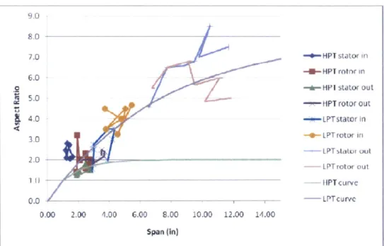
The compressor aspect ratio trend was adapted from a previous implementation of WATE and is shown in FIGURE 3-1. Fitzgerald developed the turbine trends by

examining published drawings of the calibration engines. The turbine aspect ratio

trends are shown in FIGURE 3-2.

1

Airfoil aspect ratio is defined in WATE++ as the ratio of the span to the axial projection of the blade chord. Thus, the aspect ratio controls the axial length of each blade.

4 9.0 80 7.0 6.0 5.0 4.0 3.0 2. 0.0

p

- PT rotor out -*-LPTstator in --e- L PT rotwr in LPT tatur out LPTrotor out HPT curve -LPTcurvc 0.00 2.00 1.00 6.00 8.00 10.00 12.00 14.00 Span (in)

Figure 3-2: Turbine aspect ratio variations with span[18.

3.1.2

Advanced Materials Weight Reduction Methodology

The effect of advanced materials technology on engine weight was estimated by ap-plying weight reductions to individual engine components and then recombining to get the total engine weight. The weight reductions used in Fitzgerald's models were used to develop the new engine weight models. These weight reductions, quantified as percent differences from current technology weight, were derived from published material from the MTU website, ASME and NASA publications, and communica-tions with Pratt & Whitney subject matter experts[18]. Details of the component weight reductions for advanced technology estimates are given in TABLE 3.2.

3.2

Engine Breakdown

Instead of using a single correlation to estimate the bare engine weight, the engine was broken down into five separate components for which surrogate weight models were developed. These components are a) the core, including the LPC, HPC, HPT, LPT, and their adjoining ducts as well as accessories; b) the fan, including the bypass duct;

Table 3.2: Technologies for Weight Reduction[18]

Component Current Future Weight Reduction References

Technology Technology Potential

(% of baseline)

Shafts Steel Alloys Metal Matrix 30% MTU: Steffens

Composites and Wilhelm

Fan Blades Composite, More incorporation 40-45% MTU: Steffens

Titanium of composites and Wilhelm

Fan Alloys, Composites/Kevlar 30% NASA:

CR-Containment Composites 2005-213969

Compressor Titanium/Nickel Titanium 30-40% MTU: Smarsly

Blades alloy Aluminide and P&W

Components

Compressor Titanium, Titanium Matrix 20-30% MTU: Smarsly

Disk Nickel alloy Composite Rings 2008

HPT Blades Nickel Alloy Ceramic Matrix 30-40% P&W

Composites (CMC)

HPT Disk Nickel Alloy Ceramic Matrix 30-40% P&W

Composites

LPT Blades Nickel Alloy, 50% stage 30% due to ASME

GT2003-Present Day loading increase, stage loading 38374

Stage Loading TiAl or CMC 30% due to MTU: Steffens

components TiAl or CMC and Wihelm

LPT Disk Nickel Alloy, 50% stage 30% due to ASME

GT2003-loading increase, stage loading 38374

TiAl or CMC 30% due to MTU: Steffens

components TiAl or CMC and Wihelm

Fan Drive Baseline improved 10% P&W

Gear box materials

Major Aluminum, Composites, 20-30% P&W

Frames Titanium, Ceramics

Nickel

Accessories Baseline improved 10% P&W

materials

c) the combustor; d) the nozzle, including the core and bypass nozzles; and e) the nacelle, which includes the inlet. Note that "accessories" accounts for the lubrication system, cooling system, instrumentation system, electrical system, actuation system, fuel pump and control system, and other configuration-specific items required to connect these systems to the engine2 The five component weight estimates are then

2

added together to obtain the total engine weight.

Weng = Wcore + Wjfan + Wcombustor + Wnozzie + Wnaceile (3.3)

As with Fitzgerald's weight model, current and advanced techology surrogates were developed for both the direct drive and geared fan configurations, resulting in four sets of models. The data for these models were, again, generated from several thousand WATE++ simulations varying inlet mass flow, bypass ratio (BPR), and overall pressure ratio (OPR) at SLS. The ranges over which these input parameters were varied can be found in TABLE 3.3. The range of fan pressure ratio (FPR) for

each configuration, though not a design variable, is also included in the table. The gear ratio for the geared configuration, also an output of WATE++, varied based on the stress limits of the LPT blades or the mach number limit of the LPC and ranged from 1.52 to 4.58.

Table 3.3: Design Variable Ranges for WATE++ Simulations

Variable Direct Drive Geared

Tfinlet [lbm/s] [500,3000] [500, 3000] OPR [25, 60] [25, 60]

BPR [4,15] [6,30]

FPR [1.18, 1.80] [[1.07,1.80]

Once the data were generated from WATE++ for both the direct drive and geared configurations, weight reductions were applied to the separate components following Fitzgerald's method described in Section 1.2. The final ranges of percent total engine weight for each component in the four sets of surrogate models are in TABLE 3.4. Note that the component percent total engine weights do not differ very much between current and advanced technology because the weight reductions are small compared to the component weights.

Table 3.4: Component Percentage of Total Engine Weight

Component Direct Drive Direct Drive Geared Geared

Current Tech. Advanced Tech. Current Tech. Advanced Tech. Core 45.0 - 65.3% 43.5 - 62.9% 28.4 - 57.4% 26.7 - 55.1% Fan 13.2 - 22.9% 13.1 - 22.9% 18.5 - 38.7% 18.6 - 38.9% Combustor 0.87 - 4.7% 0.88 - 4.9% 1.2 - 3.8% 1.2 - 3.9% Nozzle 7.6 - 22.1% 7.8 - 22.3% 9.9 - 26.5% 10.3 - 26.8% Nacelle 8.0 - 18.9% 8.6 - 19.5% 8.7 - 15.1% 9.2 - 15.5%

3.3

Sensitivity Analysis

Prior to developing the surrogate models, Global Sensitivity Analysis (GSA) was performed to determine the most important variables and the level of interactions between variables in the NPSS/WATE++ model. The Monte-Carlo based Sobol' method [19][20] was used to calculate the main effect sensitivity indices and total effect sensitivity indices of each variable for each engine component. The main effect sensitivity index, Si, of the ith input variable can be best understood as a measure of the variance of the system output caused by the ith variable alone, i.e. the "im-portance" of that variable. The total effect sensitivity index, ST, is a measure of the total contribution to the output variance of the system by the ith variable, including its main effect on the system plus the effects of interactions between the ith variable and the other variables. Thus, the difference between the total effect index and main effect index for a given variable is an indication of how much the variable interacts with other inputs to the system.

To calculate the sensitivity indices, 10,000 uniformly distributed quasi-Monte Carlo samples of OPR, BPR, and inlet mass flow were propagated through WATE++ to obtain component weight outputs. The input distributions were drawn from the Sobol' sequence, which is a quasi-random low-discrepancy deterministic sequence that distributes samples more uniformly throughout the design space than would a pseudo-random Monte Carlo sampling scheme. This allows the calculation of the sensitivity indices to converge with fewer samples. The process was repeated for both the direct drive and geared configurations. The block diagram in FIGURE 3-3 depicts the propa-gation of uncertainty through the NPSS/WATE++ model. The notation X ~ U(a, b)

defines X as a random variable whose value is uniformly distributed between the val-ues a and b.

OPR~- U(25,60) ,_____

BPRDD ~

U(4,15)

Component Weight

BPRG ~ U(6,30)

Distribution

minlet

Figure 3-3: Block diagram of uncertainty propagation through NPSS/WATE++.

The results of the GSA for each configuration (direct drive and geared with cur-rent or advanced technology) are plotted in FIGURE 3-4 through FIGURE 3-7. The first

figure in each set shows histograms of the output distributions of each engine com-ponent as well as the total engine weight. The second figure shows bar charts of the main and total effect sensitivity indices of each variable for each engine component. The variances given in TABLE 3.5 and TABLE 3.6 serve to illustrate the contribution

of each component to the total engine weight variance for each configuration.

For the direct drive turbofan, inlet mass flow is the most important variable to the total engine weight, as well as the core, fan, nozzle, and nacelle weights. Inlet mass flow and BPR are both important for the combustor weight. Furthermore, the com-bustor and nozzle are the only components for which there are significant interactions between design variables. As mentioned previously, the effect of interactions between one variable and the other variables is the difference of the total effect index and the main effect index corresponding to that variable. For example, from FIGURE 3-4(b),

the interaction effect for inlet mass flow on the combustor weight is the difference between the red bar and the blue bar, that is

SM,interaction = STM - SM = 0.532 - 0.445 = 0.077. (3.4)

These observations hold for both the current and advanced technology configura-tions. Only small adjustments relative to total component weight were made to the

Distribution of Core Weigh 500 400 W [] 300 200 1000 0 5000 10000 15000 Weight [ibs]

Distribution of Nacelle Weight

500 400

7 I

Distribution of Fan Weight

800

6001

Distribution of Nozzle Weigh

1000 800 a60

~

~400

Distribution of Combustor Weigh

00 600 E 401 200 0 500 1000 Weini ns] E Z

Distribution of Total Engine W eight

500 400 300 200 0 0 1 2 3 Weight [lbs x 104

(a) Uncertainty propagation for direct drive turbofan with current technology.

Sensitivities -Fan Weigh Sensitivities -Core Weigh Sensitivities -Combustor Weigh

m ain Effect M ain Effect F Main Effect

0.8 W Totai Effect 0.8 M TOtat Effect 06 Toal Effect

0.6 0.6

0.4

0.4 0.4

0.2 0 2 0.2

M OPR BPR M OPR P M OPR BPR

Sensitivities -Nozzle Weigh Sensitivities -Nacelle Weight Sensitivities -Total Weigh

*l Main Effect = Wn Effect = Main Effect

0.8

l

0.6 0.6 0.6

0.4 0.4 0.4

0.2 0.2 0.2

0 ] 0 0

M OPR BPR M OPR BPR M OPR BPR

(b) Sobol' main and total effect sensitivity indices for direct drive turbofan with current technology.

Figure 3-4: GSA results for direct drive turbofan with current technology

core, fan, and combustor weights in the advanced technology model, resulting in only small differences in variance between the current and advanced technology versions of those components.

The fact that bypass ratio is riot an important variable for the fan weight might seem non-intuitive, but this is because, in general, the NPSS/WATE++ model in-creases bypass ratio by reducing the size of the core rather than increasing the size

Distribution of Core Weigh

U

Weight libs] Distribution of Nacelle Weight

800 600 4) 400 200

0

Distribution of Fan Weight

J

(a

LO

6000

Weight [lbs]

Distribution of Nozzle Weigh

500 1000 400 800 300 E, 600 200 400 100 200 0 2000 4000 6000 0 1000 2000 3000 4000 Weight Ilbs] Weight lis]

E)

Distribution of Combustor Weigh 800 600 400 200 00 500 1000 Weight [ibs]

Distribution of Total Engine Weight

500 400 300 200 100 0 1 2 3 Weight [lbsi X10 4 (a) Uncertainty propagation for direct drive turbofan with advanced technology.

Sensitivities -Fan Weigh Sensitivities -Core Weigh Sensitivities -Combustor Weigh

1 . 1 0.8

main Effect Main Efect Main Effect

0.8 = Total Effect 08ct 0.6 Total Effect

0.6. 0.6

0.4-0.4 0.4

0.2 0.2 02

M OPR BPR M OPR BPR M OPR BPR

Sensitivities -Nozzle Weigh Sensitivities -Nacelle Weighl Sensitivities -Total Weigh

1__ ___ __ ___ __ 1

=anEfc=Main Effect =Min Effect

0.8 = Total Effect 0.8 Total Effect 0.8 = Total Effect

0M- 0.6 0.6

0.4 0.4

0.4-0.2 0.2 0.2

0 -

-M OPR BPR M OPR BPR M OPR BPR

(b) Sobol' main and total effect sensitivity indices for direct drive turbofan with advanced technology.

Figure 3-5: GSA results for direct drive turbofan with advanced technology

of the fan. It may also be surprising that overall pressure ratio is the least important variable for all engine components; this is likely because the effect of inlet mass flow overwhelms the effects of the other two variables.

For the geared turbofan, all engine components have at least two variables which

500 400 300 200 100 4) a 'a F=

o

₀

00

500 -400 300 200 100 00

Distribution of Core Weigh

10000

Weight [ibs]

Distribution of Nacelle Weight

Distribution of Fan Weight 600 400 200 0 0 2000 4000 6000 Weight lbs] 00 600 S400 200 6000

Distribution of Nozzle Weigh

.a.

Distribution of Combustor Weigh

800 600 ' 400 to- _I 200 0 0 200 400 600 800 Weight [lbs]

Distribution of Total Engine Weight 500 400 300 200 100 0 050 00 0.5 1 1 5 2 Weight [lbs] X 10 4

(a) Uncertainty propagation for geared turbofan with current technology.

Sensitivities -Fan Weigh Sensitivities -Core Weigh Sensitivities - Combustor Weigt

1 .0.8 .. 0.8

Main Effect M ain Effect

0.8 Total Effect 0.6 TotaI Effect 0 6 M Main Effect

0.6 MTotal Effect

0..4

[l

i]

0.4

0

4-0.4

0.2 0.2 0 2

M

Sensitivities - Nozzle Weigh Sensitivities - Nacelle Weighl Sensitivities -Total Weigh

1- 1 . 1

Main Effect Main Effect

0.8

**

ETotal Effect

0.6 0.6 M 6

0.4 0.4 0 .4

0.2 0.2 0.2

0 _M

ri0]11i

(b) Sobol' main and total effect sensitivity indices for geared turbofan with current technology.

Figure 3-6: GSA results for geared turbofan with current technology

are important. Additionally, bypass ratio is the dominant variable for the coinbus-tor and core weights in the geared configuration. There are also larger interactions between variables in the geared model than in the direct drive model, which can bee seen from the larger difference between the red and blue bars in FIGURE 3-6 and

FIG-800 600 400 200 0 L 0

Distribution of Core Weigh 0 L 600 400 200 10000 Weight [ibs]

Distribution of Nacelle Weight

Distribution of Fan Weight

0

Weight libs]

Distribution of Nozzle Weigh

C) E 6000 500 800 400 ₆₀₀ 0 -300 20 400 0200 100 200 0 0 2 J 02 1 0 2000 4000 6000 0 2000 4000 6000

Weight [ibs] Weight Jibs]

Distribution of Combustor Weigh

800 600 400 200 0 200 400 600 800 Weight libs]

Distribution of Total Engine Weight

500 400 300 200 100 0 0.5 1 1 5 2 Weight [ibs x 10 4

(a) Uncertainty propagation for geared turbofan with advanced technology.

Sensitivities -Fan Weigh Sensitivities - Core Weigh Sensitivities -Combustor Weigt

.ai T

Effect 0ai EEfectn ect ₀

5 0Total Effect 0.6 04 0.4 0E. 0.2

1

02

OA -d

Sensitivities - Nozzle Weigh Sensitivities - Nacelle Weighl Sensitivities - Total Weigh

1 1

EMain

MMain

0.8 Total Effect 08 MaoEect 0.8 Main Effect

LTotal Effect

0.6 0.6 0.6

0.4 04 0.4

0.2 02 0.2

0 -0 0

M OPR BPR M OPR BPR M OPR BPR

(b) Sobol' main and total effect sensitivity indices for geared turbofan with advanced technology.

Figure 3-7: GSA results for geared turbofan with advanced technology

URE 3-7 as compared to FIGURE 3-4 and FIGURE 3-5. Note that the fan weight and total engine weight for the geared configuration have larger variances than the direct drive configuration due to the larger variance in the input distribution of BPR.

800 600

E 400 200

Table 3.5: Component Weight Distribution Variances: Direct Drive Component Ocurrent [1b] gadvanced [1b]

Core 3004.8 2895.9 Fan 984.7. 975.3 Combustor 164.6 164.6 Nozzle 1248.6 1248.6 Nacelle 402.4 402.4 Total Engine 5638.7 5511.2

Table 3.6: Component Weight Distribution Variances: Geared

Component Occurrent [1b] aavanced[lb]

Core 1409.3 1386.1 Fan 1055.2 1047.8 Combustor 134.1 134.1 Nozzle 787.0 787.0 Nacelle 403.1 403.1 Total Engine 3439.4 3340.7

3.4

Surrogate Models

3.4.1

Model Types

Two types of surrogate modeling techniques were used to create the new engine weight model in TASOPT: Least Squares (LS) regression and Gaussian Process (GP) regression. LS regression fits a 2nd, 3rd, or 4th order polynomial of three variables to the data, which makes it suitable for smooth objective functions. A GP, on the other hand, interpolates the data, making it a more suitable approach for multi-modal functions. However, GPs are more computationally expensive to use and create than polynomial correlations. Most of the engine component weight functions are smooth and the LS models are sufficiently accurate. For the multi-modal engine component weight functions, a GP was used.

3.4.2

Cross-Validation

The 5-fold cross-validation method was use to validate the models presented in the following sections. In this method, the original sample data is divided into five equal

size sets. Four of the sets are used to train the model and the remaining set is used for testing. This process is repeated for all possible combinations of training and test data (five combinations). If the fit parameters and error statistics are acceptable and consistent among the five rounds, then the number of samples being used to train the model is likely to be sufficient. All of the models presented in the following sections were cross-validated with an original data set of 2500 samples. This size data set was chosen because models built using all 10,000 samples did not show any improvement in accuracy and, in the case of the GP models, took significantly more time to build.

3.4.3

Direct-Drive Turbofan, Current Materials

A full factorial design of experiments (DOE) was run in NPSS/WATE++ with eight

levels of OPR, seven levels of BPR, and six levels of rhiniet to generate 336 samples that were used to build surface plots of the objective functions. The same design variable ranges used in the GSA were used for the DOE. The fan, combustor, nozzle, and nacelle weight functions were smooth, so polynomial functions were fit to the data using the least squares method. The core weight function was multi-modal, so a GP was used instead of a polynomial fit. All models used OPR, BPR, and Tcore as input variables, except for the fan weight model, which uses minlet instead of rhcore.

Technically, these variables are interchangeable since they are related by equation,

rmcore - 1 +i-BPR, (3.5)

but since inlet mass flow is directly related to the size of the fan, a better fit was obtained using inlet mass flow as the input variable. Once the model types were chosen for each component-either a GP model or a certain degree polynomial fit-cross-validation was performed and final models were built using the Sobol' sequence samples from the GSA study. A quadratic LS model was sufficient for the combustor weight model, whereas the fan and nacelle weight models required cubic LS models. The nozzle weight had two modes, i.e. it had two peaks, and required a quartic LS model. A GP model was also explored for the nozzle weight, but maximum errors did