Developing an integrated building design tool by coupling building energy simulation and computational fluid dynamics programs

(1)

Developing an Integrated Building Design Tool by Coupling Building

Energy Simulation and Computational Fluid Dynamics Programs

by Zhiqiang Zhai M. Eng., Fluid Mechanics

Tsinghua University

Submitted to the Department of Architecture in partial fulfillment of the

requirements for the Degree of Doctor of Philosophy in the field of Building Technology

MASSACHUSETTS INSTITUTE

at the _OFTECHNOLOGY

Massachusetts Institute of Technology

_SEP1

_{7 2003}

September 2003 _LIBRARIES

Signature of Author

Department of Architecture August 1, 2003

Certified by

Qingyan Chen Professor of Mechanical Engineering, Purdue University Thesis supervisor

Certified by

Leon Glicksman Professor of Building Technology and Mechanical Engineering Thesis supervisor

C-Accepted by

Stanford Anderson Chairman, Departmental Committee on Graduate Students Head, Department of Architecture

(2)

(3)

Thesis Committee:

Leslie K. Norford, Associate Professor of Building Technology Ain A. Sonin, Professor of Mechanical Engineering

(4)

(5)

Developing an Integrated Building Design Tool by Coupling Building

Energy Simulation and Computational Fluid Dynamics Programs

by Zhiqiang Zhai

Submitted to the Department of Architecture on August 1, 2003 in partial fulfillment of the requirements for the Degree of Doctor of Philosophy

in the field of Architecture: Building Technology ABSTRACT

Building energy simulation (ES) and computational fluid dynamics (CFD) can play important roles in building design by providing essential information to help design energy-efficient, thermally comfortable and healthy buildings. However, separate applications of ES and CFD usually cannot give an accurate prediction of building thermal and airflow behaviors due to the partial modeling of the problem. An integration of ES and CFD can eliminate many of the assumptions used in ES and CFD because of the complementary nature of ES and CFD results. This thesis studies the fundamentals, implementation and application of ES and CFD coupling, significantly advancing the knowledge and experience in this area. The study has been focused on the iterative coupling of individual ES and CFD programs, which shows good potential of providing reasonable results with acceptable computing costs.

The research first analyzes the principles and challenges of ES and CFD program coupling. To bridge three major discontinuities in time-scale, spatial resolution and computing speed between ES and CFD programs, special coupling strategies have been developed. Particularly, the staged coupling strategies proposed can effectively reduce computing time while preserving the accuracy and details of the computed results.

The study discusses the solution characteristics of iterative coupling simulation. Through theoretical analysis and numerical experiments, the research verifies the solution existence and uniqueness of a coupled simulation. The investigation concludes that a converged and stable simulation can be achieved with four different data coupling methods. The study has further developed an improved iteration and control algorithm for the coupled simulation.

An integrated program, E+MIT-CFD, has been developed by coupling a new-generation ES program (E+) with a newly-developed ready-to-plug-in CFD solver (MIT-CFD). All the coupling methods and strategies proposed have been implemented in this program. The program has been well validated with various experimental facilities. The comparison of numerical solutions with experimental data reveals the advantages of the integrated simulation over the separate ES and CFD applications. The study further demonstrates the performance and capabilities of the coupled program through practical design projects. Finally, sensitivity analysis of the coupling simulation to building characteristics and coupling strategies has been performed, based on which general guidelines are established for appropriate usage of the coupling simulation.

Thesis Supervisor: Qingyan Chen

Title: Professor of Mechanical Engineering, Purdue University Thesis Supervisor: Leon R. Glicksman

(6)

(7)

ACKNOWLEDGEMENTS

I would like to express my sincere thanks to Professor Qingyan Chen, my thesis advisor, for his continuous support and guidance throughout my entire Ph.D. study at MIT. His valuable suggestions and encouragement are important to the completion of this thesis.

I would also like to thank Professor Leon Glicksman, my thesis official advisor and thesis committee chair, for his support and advisement on this thesis work.

I would also express my cordial gratitude to my other thesis committee members, Professor Les Norford and Professor Ain A. Sonin, whose valuable comments helped to improve the thesis.

My sincere thanks also extend to all my colleagues in the Building Technology Program at MIT for their collaboration and friendship.

Finally, I would like to express my special gratitude to my parents, brother, and my wife for their support, understanding and love. My special thanks will go to my lovely daughter, Sophia, who was born at MIT, for the love, hope and encouragement she brings to me.

(8)

DEDICATION

(9)

Chapter 4 Validations of EnergyPlus and MIT-CFD

50

4.1 Validations of EnergyPlus in Literatures 50

4.2 Validations of MIT-CFD 51

4.2.1 Natural Convection in an Enclosure with an Aspect Ratio of 5 51

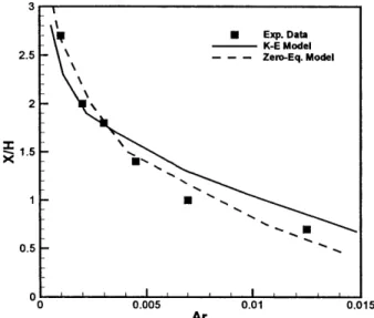
4.2.2 Forced Airflow in a Ventilated Room with an Aspect Ratio of 3 54 4.2.3 Mixed Airflow in a Ventilated Room with an Aspect Ratio of 4.7 56

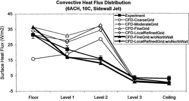
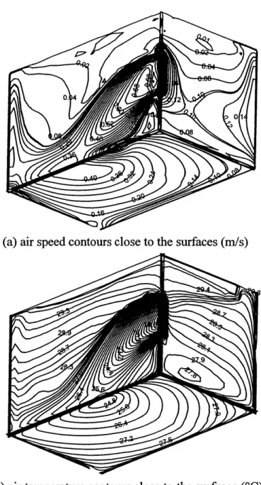
4.2.4 Three-Dimensional Airflow in a Room with Mixing Ventilation 57 4.2.5 Three-Dimensional Airflow in a Room with Displacement Ventilation 67

(10)

Chapter 5 Principles, Strategies and Implementations of EnergyPlus

and MIT-CFD Thermal Coupling

74

5.1 Coupling Principles of Energy Simulation and CFD Programs 74 5.2 Coupling Strategies of Energy Simulation and CFD Programs 79

5.2.1 Challenges for Program Coupling 79

5.2.2 Time and Spatial Coupling Strategies 80

5.2.3 Staged Coupling Strategies 81

5.3 Coupling Implementation of Energy Simulation and CFD Programs 85

5.3.1 General Rules for Developing the Coupling Program 85

5.3.2 Executive Streamline of the Coupling Program 86

5.3.3 Core Structure of the Coupling Program 87

5.4 Summary 92

Chapter 6 Determination of Convective Heat Transfer in

Simulation

6.1 Factors to Numerical Solution of Convective Heat Transfer 6.2 Theoretical Analysis

6.2.1 Convective Heat transfer in Laminar Flows 6.2.2 Convective Heat Transfer in Turbulent Flows 6.3 Numerical Investigation

6.3.1 Natural Convection along a Heated, Vertical, Flat Plate 6.3.2 Forced Convection along a Heated, Horizontal, Flat Plate 6.3.3 Natural Convection in a Room with an Aspect Ratio of 2.5:7.9 6.3.4 Three-Dimensional Airflow in a Room with Mixing Ventilation 6.4 Summary

Coupled

94 94 95 95 99 104 104 105 107 109 109

Chapter 7 Solution Characteristics of Iterative Coupling of Energy

Simulation and CFD Programs

111

7.1 Problem Statement 111

7.2 Theoretical Analysis 112

7.2.1 Solution Existence and Uniqueness of ES-CFD Program Coupling 112 7.2.2 Convergence and Stability of Iterative ES-CFD Coupling 119 7.2.3 Spatial Average Methods for ES-CFD Program Coupling 124 7.2.4 Influence of Negative Convection Coefficient on the Coupling Simulation

127

7.3 Numerical Experimentation 130

7.3.1 Case Setup 130

7.3.2 Solution Performance of Iterative Coupling Methods 131 7.3.3 Control of Indoor Air Temperature in the Coupling Simulation 135 7.3.4 Effect of Convergence Criteria on the Coupling Simulation 139

(11)

7.3.5 Effect of Control Sensor Location on the Coupling Simulation 140 7.3.6 Effect of Uniform Surface Assumption on the Coupling Simulation 141 7.3.7 Effect of Negative Convection Coefficient on the Coupling Simulation

144 7.4 Conclusions from Theoretical Analysis and Numerical Experimentation 145

Chapter 8 Case Studies: Validations and Applications

146

8.1 Cooling Load in a Room with Displacement Ventilation 146

8.1.1 Case Description 146

8.1.2 Simulation and Results 148

8.2 Natural Convection in a Room without or with a Radiator 149

8.2.1 Case Descriptions 149

8.2.2 Simulation and Results of the Room without a Radiator 150

8.2.3 Simulation and Results of the Room with a Radiator 155 8.3 Natural Convection Coefficients in a Room with a Radiator 161

8.3.1 Case Descriptions 161

8.3.2 Simulation and Results 162

8.4 Mixed Convection in a Glazed Atrium 165

8.4.1 Case Descriptions 165

8.4.2 Simulation and Results of the Atrium without Room Air Temperature

Control 166

8.4.3 Simulation and Results of the Atrium with Room Air Temperature Control 175

8.5 Ventilation System Design for a Large-Scale Indoor Auto Racing Complex 178

8.5.2 Steady Simulation and Results 179

8.5.3 Unsteady Simulation and Results 186

8.6 Displacement Ventilation in a Boston Office Building 189

8.6.2 Simulation and Results 190

8.7 Summary 196

Chapter 9 Sensitivity Analysis of Coupling Simulation

197

9.1 Coupling-Relevant Building and Environmental Characteristics 197 9.2 Sensitivity Studies of Coupling Simulation to the Building and Environmental

Characteristics 199

9.2.1 Office with Ceiling-Jet Mixing Ventilation System 202 9.2.2 Office with Side-Wall-Supply Displacement Ventilation System 209 9.2.3 Office with Floor-Supply Displacement Ventilation System 216 9.3 General Suggestions for Using ES-CFD Coupling Simulation 222

(12)

Chapter 10 Conclusions and Recommendations

227

10.1 Conclusions 227

10.2 Recommendations for Future Research 234

References 237

Nomenclature 247

(13)

CHAPTER 1

INTRODUCTION

1.1 General Statement of the Problem

Buildings, as one of the largest industries in the world, account for a major part of the total energy consumption. In the United States, building services use more than one third of the primary energy consumption and two thirds of all the electricity (U.S. Energy Information Administration 1995). The energy used by buildings drives diverse mechanical and electronic systems to achieve a convenient, efficient and comfortable environment for all kinds of human activities. Among these systems, the heating, ventilating, and air-conditioning (HVAC) system is the largest energy consumer, as illustrated by Figure 1.1. The usage of HVAC systems allows the creation of an ideal indoor environment with appropriate air speed, temperature, humidity, and contaminant concentrations, where people usually spend 80% to 90% of their time.

bqrhwwbH~m

MacDo

2%

I...

..

.

Figure 1. 1 Building energy end-use splits (US Department of Energy 2002)

However, with rising concern about the energy conservation, many efforts have been made to lessen the energy consumption of HVAC systems, for example, by using heavy insulation and a tight envelope to reduce the heating load and using a shading

(14)

system to reduce the cooling load. The development of new energy-efficient HVAC systems and technologies, such as the displacement ventilation system, can also effectively decrease the system energy consumption. The US National Renewable Energy Laboratory (NREL 1998) estimated that current building energy consumption could be reduced by 30% to 70% with all kinds of energy-efficient designs. This is very attractive because the US spends over $200 billion per year to operate residential and commercial buildings.

On the other hand, the improper design and use of building HVAC systems not only wastes energy but causes thermal discomfort and indoor air quality (IAQ) problems. For example, an inappropriate installation location of supply air diffuser may cause the circulation of the "old" air in a occupied zone. Reports of sick building syndrome and other health complaints related to indoor environments have been increasing recently. Evidence from the literature (NIOSH 1999) shows that poor indoor environments

significantly increase the rate of respiratory illness, allergy and asthma symptoms, and sick building symptoms; as a consequence, worker performance is adversely affected. A majority of studies indicate an average productivity loss of 10% due to poor indoor environment, although a conservative value of 6% is widely accepted (Dorgan et al. 1998). The overall economic losses due to the poor indoor environment in US commercial buildings is estimated to be about $40 to $160 billion per year (Fisk 2000) in lost wages and productivity, administrative expenses, and health care costs.

Therefore, it is important to assess comprehensively building performance during all the stages of building design in order to design an energy-efficient, comfortable and healthy building. Most of the building systems, especially newly-promoted systems such as double-skin fagade system, usually relate to multiple building components and involve complex interactions between indoor and outdoor environments. It is almost impossible to accurately evaluate the performance of buildings that use diverse building technologies and systems without using the help of sophisticated building design tools.

1.2 Building Energy and Airflow Simulation

Building energy simulation (ES) tools are essential for energy-efficient building design to accurately estimate building energy consumption and thermal performance. By solving the heat (and mass) transfer in the building envelopes, indoor spaces and building systems, a typical building energy simulation tool can provide:

" dynamic building envelope thermal behaviors,

" unsteady indoor environment state (temperature and humidity), " space heating/cooling load,

" capacity of the HVAC systems selected,

e energy consumption of the HVAC systems.

Numerous building energy simulation programs have been developed in the last three decades and have been widely used in the design practice as more powerful personal computers have become available. Currently, a typical hour-by-hour energy

(15)

analysis for a building in a whole year can be completed within a few seconds with a PC. Applications of ES greatly facilitate the development of energy-efficient buildings by providing a rapid prediction and better understanding of the consequences of various design decisions.

However, most ES programs assume the indoor air is completely mixed and with uniform properties. This may not be true for most buildings. The mean indoor air temperature and humidity provided by ES tools are not satisfactory for advanced indoor environment designs. Additionally, ES programs do not solve the air movement and contaminant transportation in the space. All these information are crucial to evaluate the indoor air quality and thermal comfort level of a building as well as the performance of HVAC systems.

Hence, accurate prediction of indoor environment is highly desired for the design of an energy efficient, comfortable and healthy building. Among various airflow modeling tools, computational fluid dynamics (CFD) is undoubtedly the most sophisticated airflow simulation tool. By numerically solving the governing conservation equations of fluid flows, CFD can predict the detailed time-dependent and spatial

distributions of

* air velocity in three directions (air speed), e air pressure,

e air temperature,

" relative humidity, " turbulent intensity,

* contaminant concentrations.

These results can be directly or indirectly used to quantitatively analyze the indoor environment quality and judge the system performance. For example, the air velocity, temperature, relative humidity, and the surface temperatures of building enclosures are the four most important parameters influencing indoor thermal comfort. For the evaluation of indoor air quality, the concentration level of different pollutants is the most important criterion.

Recently, CFD has played an important role in studying building thermal comfort and indoor air quality problems. Encouraging results have been achieved by using the CFD techniques for diverse indoor environmental and HVAC studies (Ladeinde and Nearon 1997, Spengler and Chen 2000). Generally, a CFD calculation for a typical room

with reasonable solution resolution may take a few hours with a modem PC (Srebric 2000).

The usage of both ES and CFD programs provides the most important parameters for the essential evaluation of building performance. Consequently, the evaluation will substantially facilitate the effort of designing an energy-efficient, thermally comfortable and environmentally friendly building with an optimal HVAC system.

(16)

1.3 Integration of Building Energy and Airflow Simulation

In the past, energy simulation has tended to be separated from detailed air movement simulation due to their different mathematical models, numerical methods, program characteristics, and modeling emphases. However, ES and CFD programs are, in fact, not independent. The information provided by these two programs is complementary. The integration of ES and CFD programs can eliminate many assumptions employed in the separate applications and result in more accurate predictions of building performance.

On one hand, air movement that ES programs do not handle has a significant influence on the load and energy estimation of a building through convective heat transfer. Most ES models use empirical formulae to generate convective heat transfer coefficients for heat convection calculation on a surface. The values may be far different from the real ones because of the dissimilarity between the case studied and the case used to produce the empirical formulae. With the development of passive cooling techniques, natural ventilation and hybrid ventilation have become more and more important in the energy-efficient building design. However, most ES programs cannot determine the accurate airflow entering/leaving a building where the room air temperature and heating/cooling load heavily depend on the airflow. In addition, the uniform indoor air temperature assumption in most ES models may not be true for some indoor spaces, such as those with displacement ventilation systems, which will also affect the accurate prediction of building energy consumption. CFD, however, can provide the detailed and accurate indoor air velocity and temperature distributions, based on which the precise convective heat transfer coefficients and convective heat flux can be calculated. The indoor air temperature gradient and convective heat transfer can then be used in an ES model for more accurate energy calculation. In addition, CFD can accurately simulate natural ventilation driven by wind effect and stack effect. The information can also be used in an ES model.

On the other hand, the accurate prediction of airflow in CFD requires accurate flow and thermal boundary conditions. In practice, most boundary conditions specified in CFD are based on measurements, empirical data or even personal experience, which may have significant adverse influence on the simulation and solutions (Awbi 1998, Emmerich 1997, Xu and Chen 1998). However, the ES results, such as heating/cooling load and wall surface temperatures, allow the possibility of providing CFD accurate and time-varying boundary conditions.

Therefore, it is attractive and beneficial to couple these two programs for the development of an integrated building design tool with best performance. One may argue that there is no need to integrate an energy simulation program with a CFD program since a CFD program can be extended to solve heat transfer in solid materials, such as building walls. With an appropriate radiation model, HVAC system model, and plant model, the extended CFD program can have the functions of both ES and CFD programs. This type of CFD program solves convective, radiative, and conductive heat transfer simultaneously. Several recent investigations (Off et al. 1996, Fisher and Rosler 1996,

(17)

Schild 1997, and Charvat et al. 2001) have attempted to use the CFD programs to analyze the dynamic performance of buildings. The approach employs CFD for the heat conduction in solid materials by the conjugate heat transfer model and uses a radiation model to consider surface-to-surface heat transfer. This allows room airflow to be calculated by prescribing boundary conditions external to the building or in adjoining spaces, rather than within the room. The method sounds powerful but it is very computationally expensive (Chen et al. 1995). The reason for the expensive computing cost is threefold:

* First, when the CFD considers the heat transfer in solid materials, the calculation becomes stiffer than the convection-only CFD. The computing time goes up dramatically in order to reach a converged and stable solution (Thompson 1988). * Secondly, since room air has a characteristic thermal response time of a few seconds

while building envelope has a few hours, the CFD simulation must be performed over a long period for the thermal performance of the building envelope but with a small time step to account for the room air characteristics. It results in the necessity for repeating the computationally demanding calculation a large number of times, providing tremendous intermediate information with which people may not even be

concern.

e Thirdly, the CFD computing time grows exponentially with building size. In small

indoor spaces with mixing ventilation of a building, the room air temperature is rather uniform and heat transfer coefficient is close to a constant. The CFD simulation is not necessary for these spaces but is still performed within the extended program.

Hence, the extended CFD (the conjugate heat transfer) method is not practical for immediate use in a design context with current computer capabilities and speed.

An alternative to reduce the computing costs in solving convective, radiative, and conductive heat transfer in both solid materials and air by CFD is to couple a CFD program with an energy simulation program. CFD handles the indoor air movement and ES solves the heat radiation between surfaces and the heat conduction in solid materials. Most ES programs deal with the heat conduction in building envelopes with various simplified methods, such as the simplification of one-dimensional heat conduction. As a consequence, the computing time of ES can be reduced to be negligibly small (seconds), compared with the computing cost of CFD that is normally a few hours for a steady calculation. Additionally, in this coupling approach, the simulation time interval of ES can be considerably large (a few minutes to an hour) because the thermal response time of solid materials in building envelopes is relatively long. CFD in this coupling approach, rather than predicting the transient airflow patterns, only simulates the indoor airflows at specific time moments with the corresponding boundary conditions obtained from ES, acting as the "snap-shots" of the airflows. Such a coupling procedure certainly saves computing time because it avoids solving the flow field during the transition from one time step to another. Furthermore, this coupling approach allows performance of CFD simulation for particularly selected indoor spaces rather than the whole building, which further reduces the computing cost.

(18)

that is equivalent to the conjugate heat transfer method, provided that the ES program subdivides surfaces reasonably small to model any significant temperature variations. Therefore, it is most interesting and attractive to directly couple ES and CFD programs, which forms the subject of this thesis work.

1.4 Research Objectives and Thesis Outline

With the long-term aim to develop an integrated building design tool in which CAD, ES, CFD and other building models are linked using standard methods, this thesis focuses on the identification of the possible roles and linkage for ES and CFD in such a tool. The thesis will discuss the potential challenges in coupling ES and CFD programs, study the possible coupling methods to the integration of ES and CFD, describe how these methods could be implemented with using a general ES and CFD program, and demonstrate the performance and capabilities of the coupled program developed.

The detailed objectives for this investigation can be summarized as: " To develop fast and practical coupling strategies;

" To study efficient and reliable iterative coupling algorithms; " To analyze solution characteristics of coupled simulations;

" To construct a compatible, flexible and easy-to-use coupling platform; " To demonstrate the applications and benefits of coupled simulations.

This thesis records the major achievements in the research and is organized as follows:

" Chapter 2 reviews the evolution of building energy simulation and airflow simulation, indicating that heat balance based ES and Reynolds-averaged CFD should be used for this coupling study. The chapter suggests the usage of a state-of-the-art ES program

- EnergyPlus (E+) developed by Lawrence Berkeley National Laboratory (LBNL)

and the development of a new ready-to-plug-in CFD solver - MIT-CFD - for this

thesis work. The chapter further reviews the current state of the ES and CFD coupling research, which enlightens the directions of this research.

" Chapter 3 introduces the fundamentals of EnergyPlus with the focus on the thermal performance of building envelope and indoor air. The chapter also discusses the

development and principles of MIT-CFD, demonstrating its good program structure and features feasible for the coupling study.

* Chapter 4 validates the MIT-CFD program via the measured data obtained from a number of classic building experiment facilities. Good agreements between the simulations and measurements verify the creditability of the CFD solver developed. The chapter also briefly introduces the validation efforts on EnergyPlus in the literature.

(19)

" Chapter 5 presents the primary principles and challenges to ES and CFD program coupling. To bridge the discontinuities between ES and CFD programs due to the different physical models and numerical methods employed, special coupling strategies are developed, in which the staged coupling strategies proposed can effectively reduce the computing costs but preserve the accuracy and details of the computed results. This chapter further introduces the general techniques employed to develop a reliable and flexible ES and CFD coupling platform.

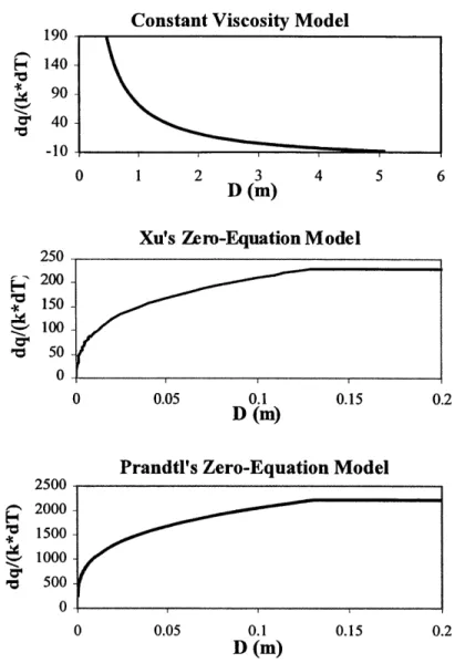
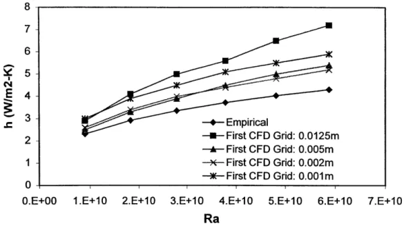
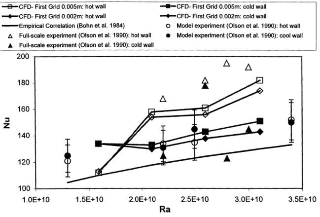
" Chapter 6 discusses the proper calculation method of convective heat transfer at enclosures, which is the key linkage between ES and CFD. The study analytically

and numerically investigates the effect of the size of the first CFD grid and turbulence model on surface convective heat transfer.

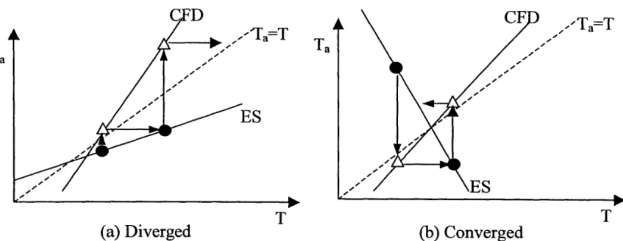
" Chapter 7 discusses the solution characteristics of iterative coupling simulation of ES and CFD programs. Through theoretical analysis and numerical experiments, the chapter addresses the concerns about the solution existence, uniqueness and correctness of the coupled ES and CFD simulation and the convergence and stability performance of the iterative coupling. The chapter also investigates the influences of some primary simulation parameters on the coupling performance.

* Chapter 8 reports the validations of the coupled program with experimental data from four full-scale building experiment facilities. The comparison of numerical solutions with the experimental data reveals the advantages of the integrated building simulation over the separate ES and CFD applications. The chapter further demonstrates the capabilities of the coupled program through two practical design projects.

* Chapter 9 discusses the building characteristics that may affect the necessity and effectiveness of the ES-CFD coupling simulation. These building characteristics along with the solution resolution requirement determine whether a coupled simulation is essential for a particular type of building and which coupling strategy can provide the best solution with the compromise of accuracy and efficiency. The chapter studies the sensitivity of coupling simulation to the building characteristics. Based on the study, the chapter provides the general suggestions for the appropriate usage of the coupling simulation.

* Chapter 10 summarizes the studies presented in this thesis and provides recommendations for future work.

(20)

CHAPTER 2 LITERATURE REVIEW

This chapter reviews the evolution of building energy simulation and airflow simulation, indicating the heat balance based ES and Reynolds-averaged CFD are most suitable for the coupling study. The review suggests the use of the newly developed ES program - EnergyPlus (E+) by Lawrence Berkeley National Laboratory (LBNL) and the development of a new ready-to-plug-in CFD solver for this research. The chapter also reviews the current state of the ES and CFD coupling research, which enlightens the directions of this thesis work.

2.1 Building Energy Simulation (ES)

Designing an energy-efficient building requires an estimate of the energy consumption in buildings. Building energy calculation methods can generally be divided into two categories: manual calculation methods and computer simulation methods. Manual calculation methods, such as the degree-day and bin methods (ASHARE 1997), are widely used in practical design due to their simplicity and efficiency, although they are not precise. Degree-day methods are the simplest methods for energy estimation and are appropriate if the building occupying and operating conditions are constant. If the conditions of the building and systems vary with outdoor temperature, the building energy consumption needs to be calculated for different values of the outdoor temperature and multiplied by the corresponding number of hours; this is the basic idea of various bin methods. More sophisticated models must be used when the situation becomes more complicated, such as varying indoor air temperature and interior heat gains. The manual methods provide a simple estimate of building annual loads, but they cannot, for example, be used for:

" evaluation of air conditioning plant.

e _{evaluation of most control issues.}

e medium or heavy weight buildings with significant diurnal fluctuations in

internal temperature.

As more powerful computers have become available, computer modeling has been more and more important for the prediction of the energy and environmental performance of buildings and systems that serve them. Computer simulation is credited with speeding up the design process, enabling the comparison a broader range of design variants and leading to optimal designs. With reasonable physical assumptions and mathematical models, the computer simulations provide more accurate and informative results than the manual calculations. As a result, it provides a better understanding of the consequences of design decisions. The underlying mathematical models and numerical schemes of simulation tools distinguish them from each other, satisfying the different requirements of complexity and accuracy.

(21)

The development of computer energy simulation programs can be traced back to the 60's and 70's, when the groundwork of energy simulation methods was laid (e.g. GATC 1967). After Mitalas and Stephenson (1967) published their milestone work on the response factor method to model the transient heat transfer through building envelopes and the heat transfer between internal surfaces and room air, ASHRAE published procedures for determining heating and cooling loads. The load calculation can then be used to size the system and compute the total energy cost.

Most energy simulation programs adopt the Load, System and Plant (LSP) modeling strategy (Sowell and Hittle 1995), which subdivides the building energy simulation into three sequential steps. The building's heating and cooling loads are first calculated for the entire analysis period (often a year) for an assumed set of indoor environmental conditions. These loads are then imposed as inputs to the second step of the simulation, which models the air handling and energy distribution systems (fans, heating coils, cooling coils, air diffusers, etc.). This second simulation step (also conducted for the entire analysis period) predicts the demands placed on the plant's energy conversion systems (boilers, chillers) and related equipment (cooling towers and circulation pumps). The third step is to calculate the source energy requirements in the central plant. Finally, one would estimate the costs of the source energy, sometimes introducing capital and other investment costs for a complete life-cycle economic analysis.

The interest of this thesis has been focused on the accuracy of the load calculation, which forms the base of the next two steps. The weighting factor method and heat balance method (ASHRAE 1997) are the two principal methods used for building load calculation in the past few decades. It is well known that heat gain is not the same as cooling load for a building. For example, the lighting energy in a room does not convert to 100% convective heat immediately. In fact, a part of the heat is radiated and then will be absorbed by the building enclosures and furniture. This part of radiative heat may be released back to the room air at a later time, because of the room thermal capacity.

The weighting factor method estimates the ratio of convective heat to the total energy release in a time sequence. The weighting factors heavily depend on building material properties, and may be pre-calculated and presented in tables for certain types of buildings. These tables can be directly used by an energy simulation program, or even manual calculation, for the load estimate if the actual building is close to the one used to produce the weighting factors. The weighting factor method was popular in the 1970s because of the limited computing capacity at that time. Earlier building energy simulation programs using weighting factors are the Post Office Program (GATC 1967), NESCAP (NASA 1975) and DOE-1 (Diamond et al. 1977).

The heat balance method was introduced in the 1970s (e.g. Kusuda 1976) to enable a more rigorous treatment of building loads. Rather than using pre-calculated weighting factors to characterize the thermal response of the room air to outdoor air temperature changes, solar radiation, and internal gains, this approach solves heat

(22)

balances for the room air and enclosure surfaces to determine the loads. The enclosure surface temperatures calculated can be used to determine the radiant temperature. The heat balance method eliminates some significant linearity assumptions and allows building dynamic conditions to be modeled appropriately. For example, the convection coefficients that characterize heat transfer from interior surfaces to the room air could respond to thermal states within the room, rather than being treated as constant. NBSLD (Kusuda 1976) is probably the earliest program of this type. Other current programs that use the heat balance method include popular ones, such as BLAST (Hittle 1979), ESP-r (Clarke 1985) and EnergyPlus (Crawley 2000).

Most weighting factor and heat balance programs use response factors (Mitalas and Stephenson 1967) and transfer functions (Stephenson and Mitalas 1971) to calculate transient conduction through walls, roofs and floors, with the assumption that the heat conduction is one dimensional. The response factors or transfer functions are based on control theory. The mathematical background is rather complicated. However, they determine heat conduction much faster than the difference method. The finite-difference method does not have to assume the one-dimensional heat conduction. It would yield much more accurate results for corner walls and would provide temperature distribution in a wall that is useful for analyzing condensation (Chen et al. 1995). However, the computing time of the finite-difference method is still considerable. Hence, most current energy simulation programs still use the response factor and transfer function methods with the fairly reasonable one-dimension assumption.

Building energy simulation has encountered incredible development since the 1970s. Recent years have especially witnessed the proliferation of building energy simulation software for a broadening range of building performance assessment. Besides the continuous improvement on the well-noticed energy software such as BLAST, DOE-2, TRNSYS, ASHRAE Loads Toolkit, ESP-r, and CODYBA (Noel et al 2001), many new energy programs are developed for research, education and design purposes, such as, ColSim (Wittwer 1999), SIMEDIF(Larsen and Lesino 2001), DOMUS (Mendes et al. 2001). To date, ASHRAE bibliography of computer simulations of building has listed more than 200 programs.

Many of these building energy simulation programs are reaching maturity - using simulation methods and even codes that originated in the 1960s. BLAST and DOE-2 are two of the most popular energy simulation programs and widely used in the building design practices throughout the world. DOE-2 (Winkelmann et al. 1993), sponsored by the U.S. Department of Energy (DOE), was developed from the Post Office program written in the late 1960s for the U.S. Post Office. BLAST (Building System Laboratory 1999), sponsored by the US Department of Defense (DOD), has its origins in the NBSLD program developed at the US National Bureau of Standards (now NIST) in the early 1970s. The main difference between the two programs is the load calculation method

-DOE-2 uses a room weighting factor approach while BLAST uses a heat balance approach. These two programs each have pros and cons and have wide utilities in various environments, but both of them have begun to show their ages in a variety of ways (Crawley 2001). The simulation methodologies in both programs are often difficult

(23)

to trace due to the decades of development (and multiple authors). To maintain, support and enhance either program, a developer must have many years of experience working with the codes, and knowledge of code unrelated to the task (due to a significant amount of "spaghetti" code). Without substantial redesign and recoding, expanding their capabilities has become difficult, time-consuming, and expensive (Crawley 2001). As a result, DOE eventually decided to start developing a new energy simulation program named EnergyPlus (E+) in 1996. EnergyPlus, developed by Lawrence Berkeley National Laboratory (LBNL), is an all-new heat balance based program with the best efforts to combine the most popular features and capabilities of BLAST and DOE-2. Compared to the legacy programs, the highlights of EnergyPlus are:

(1) simulation management structure that eliminates the interconnections between various program sections. As a result, it eliminates the need to understand all parts of the code in order to make an addition to a very limited part of the program.

(2) modularity that allows other developers to quickly add other component simulation modules with only a limited knowledge of the entire program structure.

(3) integration of loads, systems and plants that overcomes the most serious deficiency of DOE-2 and BLAST: inaccurate space temperature prediction due to lack of feedback from the HVAC module. The integration solution also allows users to evaluate a number of processes that neither DOE-2 nor BLAST can simulate well, for instance, realistic system control and interzone airflow.

Table 2.1 Comparison of major features and capabilities of three ES programs (Crawley 2001)

Features and Capabilities DOE-2 BLAST EnergyPlus Integrated loads/systems/plant solution x x

Heat balance calculation x q q

Multiple time step for interaction between x x environment, zones, and systems

Moisture absorption/desorption in building x x

envelope

Interior surface convection dependent on x temperature and airflow

Anisotropic sky model x

Advanced fenestration calculations x

Daylighting illumination and controls x

Thermal comfort model x q

User-configurable HVAC systems x x

Air and fluid loop in HVAC systems x x

(24)

Table 2.1 compares the major features and capabilities of EnergyPlus with those of BLAST and DOE-2. It is obvious that EnergyPlus is superior to its ancestors. This thesis, therefore, will use this newly developed EnergyPlus program for the coupling

study. Chapter 3 will further introduce the fundamentals of the EnergyPlus program.

2.2 Building Air Movement Simulation

Activity in the building simulation field is not limited to thermal and energy considerations. Parallel work is underway on airflow modeling. Airflow models were first developed to estimate wind and buoyancy driven infiltration effects on buildings. After that, different types of airflow models were developed to address all kinds of airflow-related problems, such as outdoor wind pressure on buildings, indoor air pollutant distributions, zone-to-zone air exchanges, natural ventilation, envelope interior surface convection, efficiency of air handling and distribution systems, etc. This study has focused on the airflow modeling of building indoor space, which is important to the building thermal comfort and indoor air quality analysis and to the building energy estimation.

Figure 2.1 shows a general classification of room airflow models. The mixing model is the simplest airflow model, which assumes the air in each single space is completely mixed and has uniform properties. It is a special case of the nodal model, and is thus also called single-nodal model in some literatures.

Mixing Model

Zonal Model

Nodal Model

Field Model-CFD Figure 2.1 Classification of room airflow models

(25)

Nodal airflow models were developed in the 1970s for simulating both infiltration and internal airflow between spaces. Nodal models treat the building and room air as an idealized network of nodes connected with flow paths. In a nodal model, a specific airflow configuration is assumed, and the mass and energy balances are written for each node of the nodal network. Lebrun (1970) was apparently the first to propose a nodal model for providing a rough estimate of thermal stratification in the context of building energy use. The work focused on modeling how heat is convected around a room by a baseboard heater under a cold window. Lebrun's pioneering work has led to the development of nodal models. Allard and Inard (1992) reviewed various levels of nodal models used in the prediction of the thermally coupled behavior of a room and its heating system. Some recent nodal models (e.g. Mundt 1996, Yuan et al. 1999, Rees and Haves 2001) can predict the vertical temperature gradient in rooms with displacement ventilation. Harrington (2001) developed a nodal model for natural ventilation where the model selects among five different airflow patterns based on the Archimedes number. The primary drawback of nodal models is that prior knowledge of the airflow patterns is required to specify mass flow in the thermal network, which makes the models difficult to use for most designers.

Zonal models introduce more flow dynamics into the prediction of mean airflows compared to nodal models. Depending on the physically valid hypotheses and experimental experience, zonal models divide the space of a room into several sub-spaces (zones). These sub-zones are combined together with the conservation of mass and energy equations. In a zonal model, air flow rates are usually solved based on temperature differences, length scales and initial momentum. Bouia and Dalicieux (1991) were apparently the first to publish what is termed a pressure-zonal model that uses pressure as a state variable and solves energy and mass balance equations in the context of building room air modeling. Inard et al. (1996) demonstrated a functional three-dimensional pressure zonal model with special cells (handlings) for walls, jets, and plumes. A difficulty in applying pressure-zonal models to most building simulations is the requirement of using special laws to describe flows in certain regions. Togari et al. (1993) presented a temperature-zonal model that was intended for use in HVAC applications for large vertical spaces such as atriums. The temperature-zonal models use empirical correlations based on temperature differences in combination with special laws for flows like jets and plumes. The main problem with temperature-zonal models is that it is difficult to obtain general-purpose convective heat transport terms that are usually developed from a small set of experiments. The recent zonal airflow models include those developed by Wurtz et al. (1998), Feustel (1998, 1999), Lin (1999), Warren (2000), Groleau and Marenne (2001), Musy et al. (2001), and Haghighat et al. (2001), as examples.

Zonal models provide increased generality compared to nodal models. Most zonal models can also be used in a personal computer and require relatively small computing power (Griffith 2002). The most attractive reason for design engineers is that limited investment and training are needed to apply these models. However, zonal models are highly experiment-dependent. The existing zonal models are limited to the predictions of mean temperature and mass flow rate in each zone. More specifically,

(26)

zonal models employ two main assumptions: (1) the primary driving flows (boundary layer, jet or thermal plume) can be pre-predicted, and (2) users have a good knowledge of the entire flow structures so that the whole flow field can be divided into zones with distinct features. These two assumptions largely limit the application of these methods in a prediction process. It is not always possible to make a clear decision about the main flow pattern. Much more work is needed to get a better knowledge of the heat and mass transfer in buoyancy-driven flows in a non-isothermal and non-adiabatic environment. Further limitations of using these models include:

" the need to quantify the driving forces and to account accurately for all openings in the room;

" the assumption of uniformly mixed air and pollutant in each zone; and " uncertainty in the results obtained with zonal models.

Beyond these, Griffith (2002) found that many zonal models are not numerically stable. Hence, it is necessary to develop and utilize more general, accurate, detailed, and stable air movement models.

With the development of fluid mechanics and numerical methodologies, the computational fluid dynamics (CFD) technique has been a popular tool for predicting engineering flows since the early 1970's. CFD is receiving greater acceptance as a technique for building airflow analysis. It offers the potential of much richer details, a higher degree of flexibility, and lower cost than the traditional laboratory study. As the most sophisticated airflow model, CFD provides the detailed spatial (field) distributions of air pressure, velocity, temperature, humidity, contaminants, and turbulence intensity by solving the conservation equations of mass, momentum, energy, and species concentrations. The air velocity, temperature, relative humidity, and the surface temperatures of building enclosures are the four most important parameters influencing thermal comfort of indoor space. The concentration level of different pollutants can be directly used to evaluate building indoor air quality. In addition, Fanger et al. (1989) pointed out that turbulence intensity has a significant impact on draft. Hence, CFD results assist the quantitative analysis of the thermal comfort and indoor air quality status of a building in great detail.

Nielsen (1974) was probably the first one who applied CFD techniques to room air motion. Applications of CFD for room airflow were mushrooming in the 1980s. The International Energy Agency Annex 20 was particularly devoted to room airflow prediction with participants from 13 countries (Moser 1994). In the past two decades, numerous encouraging results have been achieved by using the CFD technique for studies of building thermal comfort and indoor air quality, as reviewed by Whittle (1986), Liddament (1991), Jones and Whittle (1992), Chen and Jiang (1992), Moser (1992), Lemaire et al. (1993), Emmerich (1997), Nielsen (1989, 1998), and Spengler and Chen (2000). Ladeinde and Nearon (1997) reviewed CFD applications in the HVAC industry. These reviews concluded that CFD is powerful in predicting building air movement, although users' knowledge, experience and skills with CFD are essential to the accuracy of CFD results.

(27)

The airflows that CFD predicts can be laminar, turbulent, or transitional between laminar and turbulent flows. Turbulence is characterized as chaotic state of fluid motion, which most real flows are. As yet no complete theory on turbulence exists, because its nonlinear dynamics is not well understood. Due to the sophisticated characteristic properties of turbulence, such as irregularity, nonlinearity, diffusivity, large Reynolds numbers, three-dimensional vorticity fluctuations, dissipation and continuum (Tennekes and Lumley 1972), it is difficult to identify whether airflow in a room is a locally artificially induced, transitional, or fully developed turbulence. However, very few room airflows are laminar. All non-laminar room airflows could be defined as turbulence. CFD prediction on turbulent flows currently is by three approaches: direct numerical simulation (DNS), large-eddy simulation (LES), and Reynolds-averaged equations simulation with turbulence models.

DNS computes a turbulent flow by solving the highly reliable Navier-Stokes equation without approximations. DNS requires a very fine grid resolution to capture the smallest eddies in the turbulent flow. According to turbulence theory (Nieuwstadt 1990), the number of grid points required to describe turbulent motions should be at least N -Re94_{. The computer systems must become rather large (memory at least 1010 words and}

peak performances at least 1012 flops) in order to do computations for the flow (Nieuwstadt et al. 1994). In other words, since the smallest eddy size in a room is about 0.01 m to 0.001 m, at least 1000 x 1000 x 1000 grids are needed to solve the airflow. Neither existing parallel computers nor computers of the near future can even approximately supply the storage space or the necessary CPU performance demanded by such a simulation. In addition, the DNS method requires very small time steps, which makes the calculation extremely time consuming. It is clear that in the near future the applications of the direct numerical simulations for indoor flows are not realistic.

Deardorff (1970) developed a method named "large-eddy simulation" with the hypothesis that the turbulent motion could be separated into large-eddies and small-eddies such that the separation between the two does not have a significant effect on the evolution of large-eddies. The large-eddies corresponding to the three-dimensional time-dependent equations can be directly simulated on existing computers. Turbulent transport approximations are then made for small-eddies independently from the flow geometry, which eliminates the need for a very fine spatial grid and short time steps. The philosophy behind this approach is that the macroscopic structure is characteristic for a turbulent flow. Moreover, the large scales of motion are primarily responsible for all transport processes, such as the exchange of momentum and heat. The success of the method stems from the fact that the main contribution to turbulent transport comes from the large-eddy motion. Thus the large-eddy simulation is clearly superior to turbulent transport closure wherein the transport terms (e.g. Reynolds stresses, turbulent heat fluxes, etc...) are treated with full empiricism. LES has been successfully applied to several building indoor and outdoor airflow studies. Some examples of such applications are the flow around a building (Murakami et al. 1996), forced convection flow in a room (Davidson and Nielsen 1996, Emmerich and McGrattan 1998), natural ventilation flow in buildings (Jiang and Chen 2001), and particle dispersion in buildings (Jiang and Chen 2002). Murakami (1998) concluded that LES can produce accurate results both at the

(28)

mean and turbulent levels for airflows in and around buildings. However, LES needs large computer power and memory because of the required fine grid and unsteady calculation. Jiang (2002) indicated that LES even with an empirical model, such as a wall model, to reduce the grid number in the near-wall regions, requires 4-5 days of computing time with a fast workstation for a wind-driven airflow. For the simulation of buoyancy-driven airflows, more computing time is needed. This is not acceptable for most building design purposes. With the development in computer capacity and speed, LES may be used as the main tool to building airflows in the future.

Since the details of turbulent flow are difficult to model and engineers are mainly interested in the mean values, one then turns to solving the Reynolds-Averaged Navier-Stokes (RANS) equations with turbulence models. In the RANS approach, CFD treats flow dynamic quantities as some sort of statistically averaged (Reynolds-averaged) turbulent field and simulates merely the gross features of the turbulent flow. The turbulence fluctuation effect on the mean airflow can be represented by different turbulence models. Turbulence models are simplified mathematical descriptions of turbulent flows. They are based on good physical insight, and are applicable to complicated flows encountered in reality. With a turbulence model, it is possible to predict the flows found in practice with the capacity of present computers. Many turbulence models have been developed in the last century, which can be generally divided into two categories: eddy-viscosity models and Reynolds stress models.

The eddy-viscosity models adopt Boussinesq approximation (1877) that relates Reynolds stress to the rate of mean stream through an "eddy" viscosity. Classic eddy-viscosity models include mixing-length model (zero-equation eddy-eddy-viscosity model) (e.g. Prandtl 1926), one-equation eddy-viscosity model (e.g. Kolmogorov 1942), and

two-equation eddy-viscosity model (e.g. Launder and Spalding 1974).

The zero-equation eddy-viscosity models are the simplest turbulence models. The model has one algebra equation for turbulent viscosity, and no (zero) additional partial differential equations beyond the Reynolds-averaged equations for mass, momentum, energy, and species conservation. Hence, it has the best computing efficiency. Although zero-equation models have fatal physical deficiency, for instance, without considering non-local and flow-history effects in the eddy-viscosity, and although more sophisticated turbulence models are developed, zero-equation models still gain certain attentions in today's industrial practices because they are simple, cost-effective, and once calibrated, can predict mean-flow quantities fairly well. In fact, some simple zero-equation models may provide surprisingly good results. For example, a constant viscosity model (an empirical constant v,) can give much better results for swirling flow than the standard k-s model. Alk-so, Nielk-sen'k-s k-study (1998) k-showed that the conk-stant eddy-vik-scok-sity model provides results closer to the measured data than the standard k-s model for the prediction of smoke movement in a tunnel. Xu (1998) developed a zero-equation model, which was demonstrated to have the high feasibility in predicting room airflows by many validations such as Chen and Xu (1998), Srebric et al (1999), and Beausoleil-Morrison (2000).

(29)

(1974), so-called "standard" k-c model, has been widely used in practice, where k is turbulence kinetic energy and , is the dissipation rate of turbulence energy. Numerous other two-equation models have been suggested afterwards. Chen (1995) has tested five different k-E models for natural convection, forced convection, mixed convection and impinging jet in a room, but it is very difficult to identify any other models superior to the standard k-s model.

The Boussinesq approximation is sometimes inadequate to represent the local state of turbulence for complex flow situations, such as recirculating flows in a room. This deficiency can be overcome in Reynolds stress models (RSMs) that explicitly employ transport equations for the individual Reynolds stresses. Although the study of RSMs has been started in the 1970s, the applications of RSMs toward three-dimensional flows began to appear in the 1990s. Direct applications in room airflow computation include those by Murakami et al. (1990) and Renz and Terhaag (1990). They computed airflow patterns in a room with jets. The results show that the RSM is superior to the standard k-s model, because anisotropic effects of turbulence are taken into account. Chen (1996) compared three RSMs with the standard k-S model for natural convection, forced convection, mixed convection, and impinging jet in a room. He concluded that the RSMs are only slightly better than the k-c model but have a severe penalty in computing time. Based on a large number of applications for engineering flows, Leschziner (1990) concluded that RSMs are appropriate and beneficial when the flow is dominated by a recirculation zone driven by a shear layer. Thakur and Shyy (1999) reviewed the latest status of Reynolds stress models and the various associated modeling issues. The review confirmed the importance of RSMs for the flows involving strong streamline curvature due to the geometry complexity or a high degree of swirl. However, the implementation and application of RSMs are not a trivial task - it brings with it a number of issues associated with the stability of the overall algorithm and boundary conditions. The simulations with RSMs requires (three to ten times) more computing time than those with eddy-viscosity models because of greater algebraic complexity. Additionally, although with the continuous development (e.g. Craft 1998, Hanjalic and Jakirlic 2002), the RSMs still have various defects and weaknesses, especially for low-Reynolds and buoyancy-driven airflows. Hence, the models need further study, improvement and validation before they can be widely used for room airflow prediction.

Most of today's CFD programs used in practice solve the Reynolds-Averaged Navier-Stokes (RANS) equations with different kinds of eddy-viscosity turbulence models, which provides reasonably accurate results with acceptable computing costs. To satisfy the building design purpose that mostly focuses on the macro-level characteristics of flow and heat transfer and requires fast simulation responses, the present study should adopt the RANS simulation approach using several simple and classical turbulence models for room airflows, i.e. constant viscosity model, zero-equation model (Xu 1998), and standard k-E model (Launder and Spalding 1974).

Many commercial CFD software have been developed in the last two decades. Some of them are even specially developed for building industry applications, such as AirPak (Fluent 2001). However, most commercial CFD programs are usually difficult to

(30)

integrate into the whole building simulation program because of its huge code size and complicated program features for versatile simulation purposes. Existing research CFD programs also require major modifications, sometime even re-organization of the entire program structure, before they can be plugged into a building simulation program. Therefore, the present investigation will develop a new CFD solver, MIT-CFD, for the coupling with the EnergyPlus program. The program will use the standard CFD techniques and can predict building room airflows with a reasonable accuracy and computing speed. The highlights of the program will be the well designed and implemented data and program structures that allows the easy plug-in of the program to an arbitrary building energy simulation program. Chapter 3 will present the fundamentals, development and features of this CFD program.

2.3 Integration of Energy Simulation and CFD Programs

Building energy simulation and CFD programs provide important and complementary information for the evaluation of building performance. Due to their different modeling emphases and methodologies, these two programs are usually applied separately. However, in the past ten years, efforts have been made to combine these two aspects. This is because the integration of ES and CFD allows the elimination of many assumptions used in separate ES and CFD and results in more accurate and detailed predictions of building performance. On one side, the energy simulation of a building, a complicated system, requires the concurrency of many physical phenomena. Particularly, the air movement has the most significant influence on the convective heat transfer, and therefore the energy estimate of a building. On the other hand, the airflow simulation by CFD requires the enclosure surface temperatures and supply heating or cooling energy as inputs, which can be obtained from the energy simulation.

Chen (1988) was probably the first one to try to couple an energy simulation program with a CFD program. In his approach, the CFD program solves the convective heat transfer and airflow in a room. An energy simulation program simulates radiative and conductive heat transfer in buildings. The outputs of the energy simulation program, such as wall surface temperatures and loads, are the inputs of the CFD program. On the other hand, the results of the CFD program, such as room air temperature distribution and convective heat transfer coefficients, are the inputs of the energy simulation program. With this coupling approach, the computing costs are much cheaper than that with a conjugated CFD program, while reasonable solutions are still achieved. Limited by the computer capacity available at that time, manual/static coupling was conducted in his study. Chen also proposed some other measures to further reduce the computing costs, such as using a few fixed airflow patterns to calculate hour-by-hour air temperature distribution.

Srebric et al. (2000) improved Chen's study (1988) by automatically/dynamically coupling a CFD program with an ES program for building heating/cooling load calculation. The simulations show the explicit benefits from the coupling, as Nielsen and Tryggvason (1998) confirmed that an interconnection between a CFD program and a