Coupling building energy simulation and computational fluid dynamics: Application to a two-storey house in a temperate climate

1

Coupling building energy simulation and computational fluid dynamics:

application to a two-storey house in a temperate climate

Mathieu Barbason, Sigrid Reiter

Mathieu Barbason – Corresponding author

LEMA, Université de Liège, Chemin des Chevreuils, 1, 4000 Liège, Belgium. Phone number: +32 4 366 9360

Fax number: +32 4 366 2909 Mail: mbarbason@ulg.ac.be Sigrid Reiter

LEMA, Université de Liège, Chemin des Chevreuils, 1, 4000 Liège, Belgium. Phone number: +32 4 366 9482

Fax number: +32 4 366 2909 Mail: sigrid.reiter@ulg.ac.be

2 Abstract

This article reports the coupling of a building energy simulation (BES) with computational fluid dynamics (CFD) software and its application to a typical Belgian two-storey house. The coupling scheme developed in this study aims to improve the overheating prediction for buildings. This phenomenon is becoming increasingly frequent in Northern Europe due to increased insulation and a lack of sun protection and natural cooling strategies. Complementary contributions of the two numerical approaches are underlined and used to obtain accurate results in an acceptable computing time, even in a thermally stratified room. The space and time coupling is discussed to obtain an optimised tool in which BES is in charge of the primary portion of the effort, while CFD intervenes punctually on one room of interest. The numerical results are compared both qualitatively and quantitatively to the experimental results, and the improved accuracy of the coupled tool compared with a standalone BES is underlined.

Keywords: computational fluid dynamics, multizone model, building physics simulations, validation, overheating risks.

3 1. Introduction

The reduction of a building’s energy consumption has become one of the most challenging goals worldwide. This problem is especially challenging in Europe, where 40% of the total energy is dedicated to the heating and cooling of buildings [1]. Therefore, building designers are urged to use new strategies to develop near-zero energy buildings. In fact, European regulations will impose the building of zero-energy buildings as soon as 2020.

The scientific community has developed several approaches for building energy simulations (BES) to help building designers, such as multizone dynamic simulations. Moreover, aeronautical studies have yielded parallel computational fluid dynamics (CFD) models that could be applied to building cases. These approaches aim to optimise building design and retrofitting. Nevertheless, they have a number of limitations and drawbacks.

BES is widely used due to its ease and speed. Chen [2] shows that multizone models have been the main tools for predicting ventilation performance in an entire building over the past years. The multizone model allows the prediction of overall flow through the building and the prediction of mean temperature in small rooms, but it cannot predict detailed temperature and airflow distributions within each room. Specifically, the multizone approach assumes the perfect mixing of the air in each zone, which generally corresponds to a perfect mixing of air in each room. Thus, this approach suffers from a lack of accuracy for thermally stratified rooms. However, recent architectural designs have developed massively glazed buildings and atrium configurations. This type of configuration significantly increases the risk for overheating and thermal stratification in large or high rooms. Thus, multizone models are not reliable for this type of building. Some studies have already extensively discussed the multiple assumptions and drawbacks of the multizone model [3-5].

4

Conversely, computational fluid dynamics software has already proven its ability to accurately model all types of aero-thermal phenomena in buildings and their surroundings, such as mechanical ventilation [6-8], natural ventilation [9, 10], contaminant dispersion [11, 12], airflow around buildings [13], heat islands [14], etc. Chen [2] shows that CFD models have been mainly applied to study indoor air quality, natural ventilation and stratified ventilation because these phenomena were difficult to predict via other models.

As the most sophisticated airflow model, CFD simulations can provide detailed spatial distributions of air velocity, temperature and contaminants in each room. Unfortunately, they suffer from long calculation times, especially for highly partitioned buildings, which limit their adoption by practitioners. Moreover, Li and Nielsen [15] argue that large efforts must be devoted to raising awareness on the reliability of these techniques, defining good practice rules and helping new operators to suitably use these techniques. Several recent studies have attempted to address this issue, especially in terms of the selection of turbulence models [6, 16-18].

To meet the needs of building designers, the scientific community has studied the complementarity of these two tools: the ease and speed of the multizone approach and the accuracy of CFD. These efforts yielded simulations that couple BES and CFD. The coupling allows operators to exploit the qualities of each approach. However, this requires overriding three major discontinuities between the two techniques [19]:

1. Spatial discontinuity meshes are completely different;

2. The temporal discontinuity: the multizone approach can easily be used to conduct studies over an extended period of time (several months to a year calculated per time step of an hour), while the CFD solves simulations over relatively short periods (a few hours, calculated per time step of a second);

5

3. Discontinuity of computation time between the two approaches.

This article aims develop a coupled BES-CFD approach that is optimised for overheating predictions in complete buildings. An application of this tool to a Belgian residential building (two floors and 11 rooms) on a sunny summer day will allow its numerical results to be compared with experimental measurements in the studied house, as well as with the numerical results of a standalone BES simulation. This article is structured as follows: Introduction, State of the art of BES-CFD coupling, Case study description, Developed coupling tool description, Simulation parameters of the case study, BES standalone results, Coupled results and Conclusions.

2. BES-CFD coupling – State of the art

The idea of coupling BES and CFD was first developed by Negrao [20], who focused on the necessity for the two models to exchange appropriate boundary conditions. Indeed, CFD requires surface temperature to accurately describe the flow condition, but these values are unknown at the design stage. Conversely, BES requires convective heat flux coefficients for each wall and thermal gradients description within rooms with high vertical development. This study developed 3 models. In the first one, the two approaches run in parallel without direct interaction. In the second one, BES provides the surface temperature to CFD, while CFD supplies convection heat transfer fluxes. Finally, this study attempted to add an aeraulic parameter to its coupling

approach. Unfortunately, this last technique was not a success.

Zhai et al. [19] reviewed several coupling approaches and classified them based on their coupling iterative process and the number of data exchanges between the two tools. In a static coupling, the study focuses on one particular moment of interest for which BES generally provides wall temperatures to CFD. A reverse data exchange, from CFD to BES, may also help to improve accuracy. In a dynamic coupling, BES and CFD exchange useful data at several time steps to

6

capture the transient phenomena. Zhai et al. [19] considered 4 exchange protocols that will be explained in detail hereafter. Finally, they applied these different schemes to two single room cases. They underlined that a coupling approach can significantly improve the cooling/heating loads and comfort predictions.

Zhai and Chen [21] verified the existence, uniqueness and convergence of a solution obtained by a coupling approach based solely on thermal aspects. They tested several exchanges parameters (such as convective heat transfer coefficients or heat fluxes from CFD to BES). Finally, they claimed that the most stable approach was to transfer the surface temperature from BES to CFD and convective heat transfer coefficients from CFD to BES.

Wang and Chen [22] have expanded on the study of Zhai and Chen [21] to include aeraulic parameters. They claimed that the stable approach consisted of exchanging the pressure boundary conditions between BES and CFD and vice versa. Wang [23]pursued the development of this approach by studying contaminant dispersion in a four-room case. He demonstrated that a coupling approach yields more realistic results than standalone BES software. In parallel, Djunaedy et al. [24] noted that internal coupling (in which BES and CFD are assembled in one single tool) has limitations that can be overcome by the use of an external coupling (in which BES and CFD work sequentially). This approach drastically decreases the computing time and improves the accuracy of results.

Finally, Pappas and Zhai [25]studied the performance of a double skin cavity with a coupled BES-CFD programme: the model was validated using measured data, and errors were calculated for airflow rate prediction (9%) and for temperature stratification (15%).

In this frame, our study aims to demonstrate that a coupling approach can easily be applied to a complete building (two floors and 11 rooms), including an open space with high air temperature

7

stratification. This approach accurately predicts the overheating phenomenon. This problem is becoming increasingly prevalent, and building designers do not have efficient tools to predict overheating. The developed tool is based on an external and dynamic coupling that addresses thermal and aeraulic aspects.

3. Case study description

The chosen case study is a typical Belgian house from the 1990s composed of two storeys with an entrance hall with a stairwell, a living room, a kitchen, a laundry and a professional office at the ground floor and a personal office open on the entrance hall and stairwell, four sleeping rooms and two bathrooms at the first floor. The two storeys are linked by the entrance hall, which also fulfils the role of personal office on the upper level (Figure 1). This room is often the only office of this type of house. Therefore, ensuring good thermal conditions in the upper part of this room is important. For simplicity, we refer to this space as “the open space” in the rest of the article.

8

9 thermal sensors were placed inside this room to measure the thermal gradient due to

stratification (Figure 2). The sensors were placed at a vertical distance of 60 cm from the first sensor, which was placed 10 cm from the floor. The temperature at the centre of each room of the house was also monitored to evaluate both the multizone and the CFD parts of the simulation. Additional sensors were also placed in several rooms to ensure the thermal uniformity of the rooms that are modelled by BES. The external temperature was also monitored, and the results were compared with the nearest airport readings.

The measuring campaign persisted for three entire days, with a measuring time step of 2 minutes. The measuring accuracy was +/-0.35°C between 0°C and 50°C.

A blower-door test was used to evaluate the permeability of the house. According to the

Norm EN 13829, the air renewal rate was approximately 5.5 volumes per hour under a pressure difference of 50 Pa between the inside and the outside. This value is characteristic for a mid ‘90s house that is not equipped with mechanical ventilation.

Finally, to ensure that the coupling approach can predict overheating, the measurements were conducted during a hot and sunny period.

9 Figure 2: Sensors implantation inside the open space

4. Developed coupling tool description

Limiting the CFD interventions to strictly necessary steps is important to ensure an efficient and fast approach. Indeed, CFD calculations are time- and resource-consuming. Therefore,

Negrao [20] noted that space discretisation was an important factor and that it was possible to separate the building in two parts: one in which the air property gradients are crucial, which has to be modelled by CFD, and another in which the air can be considered well mixed, where the multizone approach is most suited. Following the same efficiency goal, Zhai et al. [19] proposed to limit CFD interventions to a reduced number of time steps. Thus, BES provides the main calculation effort, and the calculation time is drastically reduced.

This section describes the choices made during the development of our coupling tool in terms of spatial discretisation, temporal discretisation, the coupling scheme and the developed algorithm.

10

4.1 Space discretisation

As already noticed by Negrao [20], the ability of BES to accurately predict the thermal behaviour of small rooms is well known. In these rooms, the air is well mixed, and the air properties (such as temperature) can be considered as constant in the entire room. Because these rooms do not present large thermal gradients or substantial convective transfer, they are eligible for a BES approach.

Conversely, the CFD domain must be reduced as much as possible to limit computing time, as this technique is very time consuming. Space discretisation for CFD requires a fine grid over which the density, air velocity and temperature are calculated via Navier-Stokes equations. The required computing resources grow quickly, and simulations can last several days if this aspect is not considered.

Therefore, only the open space was modelled with CFD, while BES was used to model the remaining house (10 rooms). Given the vertical development of the open space and the fact that the front wall is glazed, this area is subject to thermal stratification, while all the other rooms are small and experience small thermal charges. Moreover, the open space temperature prediction is very important due to its central role and effect on all other rooms (except the laundry).

4.2 Time discretisation

Because overheating is a transient phenomenon, a dynamic coupling approach was necessary. Zhai et al. [19] noted several possible coupling approaches, which can be summarised by the following rules: one-time step dynamic coupling, in which coupling is applied for one specific time-step of interest; quasi-dynamic coupling, in which the effort is supported by BES and CFD takes punctual action; full dynamic coupling, in which BES and CFD alternate towards a

11

converged solution for each time step, and virtual dynamic coupling in which specific time steps are modelled with both BES and CFD, the results of which are interpolated in an extended-time simulation.

In this paper, quasi-dynamic coupling was used because it represents the best compromise between accuracy and calculation time for a building. The coupling approach choice depends strongly on the impact of transient phenomena on the thermal behaviour of a room. Because solar illumination is the main transient phenomenon in our case, an entire CFD simulation at every time step is not necessary. In other words, quasi-dynamic coupling can accurately model configurations without dramatic thermal changes, such as the conditions of a Belgian house in summertime.

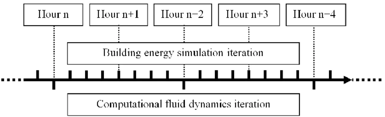
Thus, BES simulates the thermal behaviour of the house on an entire day with a quarter-hour time steps, and the CFD simulation provides inputs every two simulated hours in our model (Figure 3).

Figure 3: Time discretisation scheme

An initialisation process was necessary. To this end, BES models the two previous days, while the first CFD first occurs two hours before the day of interest. Thus, 13 total CFD calculations based on the results of each of the last CFD time step to decrease calculation time. The final coupling scheme is illustrated in Figure 4.

12 Figure 4: Space discretisation scheme

4.3 Coupling scheme

BES-CFD coupling is increasingly used to consider both thermal and aeraulic aspects because they are increasingly modelled in parallel to BES. This approach was retained for this study because it is the most accurate.

The internal surface temperatures were transferred from BES to CFD. In the reverse direction, CFD supplies the heat transfer coefficients. This approach ensures stability and convergence, as demonstrated by Wang and Chen [22]. In addition, CFD also provides the near-wall temperatures because the space domain has been completely merged. The possibility to refine the temperature in the vicinity of each wall (and not the temperature of the whole room) in the BES model, which is attributed to CFD, should thus increase accuracy.

The mass flow was transferred from BES to CFD, while the mean temperature by storey was reversely provided to consider pressure variations due to stratification in the reverse direction. This approach differs from the recommendation of Wang [23], as the space domain was not merged in these test cases. The developed coupling scheme is reproduced in Figure 5.

13 Figure 5: Coupling scheme

4.4 Developed algorithm

A coupling programme with a text-mode interface was developed between TRNSYS and Fluent. This text-mode data exchange interface was programmed in the C++-language to provide a

14

convenient data passage between TRNSYS and Fluent that automatically implements the data exchange between the two programmes.

5. Simulation parameters of the case study

In a complete validation process, ASHRAE [26] recommends that the main simulation

parameters be described to permit the reproduction of the simulation by anyone. To this end, this section introduces the main parameters of the coupling approach simulation.

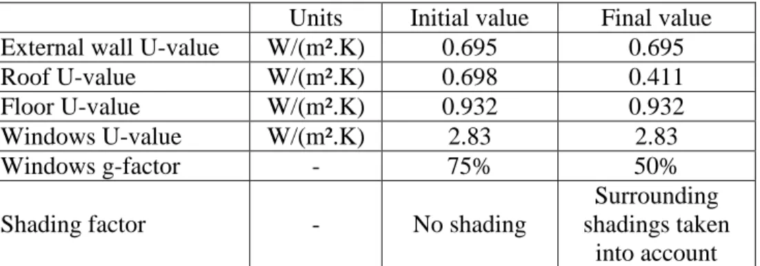
Table 1 illustrates values that were retained for the BES part of the simulation. Moreover, it also introduces the evolution of the parameters during the calibration process by providing the initial and the final values of these parameters.

Table 1: BES main parameters

Units Initial value Final value External wall U-value W/(m².K) 0.695 0.695

Roof U-value W/(m².K) 0.698 0.411

Floor U-value W/(m².K) 0.932 0.932

Windows U-value W/(m².K) 2.83 2.83

Windows g-factor - 75% 50%

Shading factor - No shading

Surrounding shadings taken

into account

A 195,990 polyhedral cell mesh was initialised for the CFD model, which represents a typical length scale of 7.5 cm for the cells. This mesh is somewhat smaller than the recommended value of Nielsen et al. [27], which is a mesh of approximately 240,000 cells mesh given the volume of the open space. Nevertheless, the convergence of results was verified, and our mesh was

optimised to decrease the computing time as much as possible.

15

boundary conditions) was used as recommended by Cook and Lomas [28] to optimise the convergence of results. The simulation was decomposed in two parts with respect to the time step. During the first part, the time step was 20 seconds, which permits a first approximation of the results. During the second part of the simulation, a 2-second time step was used to refine the quality of results.

The turbulence model is a SST k-w model. Indeed, this model yielded the more satisfactory results in this specific case in comparison with the k-ε models. Solar radiation was modelled with a P1 solar model, which is the best compromise between accuracy and calculation speed.

Finally, several concerning discretisation schemes were employed. The pressure extrapolation scheme was a PRESTO model, the pressure-velocity coupling scheme was a SIMPLEC model, the gradients and derivatives were evaluated with a Green-Gauss Cell Based model and a second order model was used to extrapolate the other variables (velocity, energy, etc.). These parameters were selected based on the results of an optimisation process on the quality of results.

6. BES standalone results

The BES software retained for this study was TRNSYS [29]. Crawley [30] proved that this multizone programme is most suited for a BES-CFD coupling approach. This software has the advantage of being very flexible and widespread use by building engineers offices.

As it is often the case with real case studies based on in-situ measurements, some parameters were uncertain, such as the current U-value or g-factor of windows. Therefore, BES was first performed on the entire house during the three studied days to calibrate uncertain parameters and obtain a correct starting point for the BES-CFD coupling approach evaluation.

16

To this end, the quality of results was evaluated via a linear regression approach. This technique consists of plotting the experimental results versus the numerical results. A linear interpolation of the results was then applied. This operation defines a slope coefficient, which must fall inside the range of [0.75, 1.25], and a correlation coefficient R², which must exceed 0.9 [26]. The first indicator reflects the accuracy of the modelled temperature range, while the second one tests the correctness of the time evolution.

Linear regressions were calculated separately and in groups for the 10 small rooms, and the results of the optimisation parameters are described in Figure 6 for the slope coefficient and in Figure 7 for the correlation coefficient.

17

Figure 7: Optimisation process: correlation coefficient R² (target interval: [0.9,1])

The figures show that results are favourable at the beginning only for Bathroom 1. The results are outside the acceptable range for Bedroom 1, Professional Office and Laundry. Moreover, the correlation with all the available data (total curve) is also outside the acceptable range.

Uncertain parameters, such as the g-factor of windows or U-value of the insulation, were modified, and correct results were finally obtained after 10 iterations. In the last iteration, the correlation coefficient R² for the 10 grouped rooms was 0.924, and the slope coefficient was 0.939. Compared with the recommendation of ASHRAE [26], these results are good and the simulation parameters can be considered correctly calibrated. The changes in the slope coefficients and the correlation coefficients R² are given in Table 2.

Table 2: Optimisation parameters evolution

Correlation coefficient R² Slope coefficient

Initial value Optimised value Initial value Optimised value

Sleeping Room 1 0.81 0.92 1.18 1.02

Bathroom 1 0.93 0.92 1.02 0.98

Laundry 0.85 0.98 1.12 1.04

Professional office 0.87 0.95 1.32 1.15

18

The results indicate that all parameters conform to ASHRAE recommendations and that the improvement of the results of initially faulty rooms does not affect the results of Bathroom 1, which were accurate from the beginning.

6.1 Small rooms results

The finals results of the change in the average temperature of four rooms (2 per storey) during 24 hours are described in Figure 8. These results illustrate the accurate prediction of the temperature in these four rooms. The mean error is an underestimation of 0.1°C, and the absolute mean error is approximately 0.5°C, which represents 5.8% of the encountered temperature range. Similar results were obtained for the other 6 small rooms.

0 10 20 24 26 28 30 32 Laundry Te m p e ra tu re [ °C ] Daytime [h] 0 10 20 24 26 28 30 32 Bedroom 1 Te m p e ra tu re [ °C ] Daytime [h] 0 10 20 24 26 28 30 32 Bathroom 2 Daytime [h] Te m p e ra tu re [ °C ] 0 10 20 24 26 28 30 32 Kitchen Te m p e ra tu re [ °C ] Daytime [h] Experimental results Numerical results

19

This type of result was expected, because the multizone approach is known to perform well when the air properties, such as temperature, are uniform inside the room, as is the case in the studied rooms.

6.2 Open space results

Conversely, the open space results are inconsistent, as illustrated in Figure 9. The simulated temperature overestimates the maximum registered temperature during 5 hours in the morning. Moreover, the BES maximum temperature occurs 2 hours before the maximum registered temperature and underestimates the peak value by 1.5°C. Thus, the BES results are physically inconsistent for the open space, and BES is not suitable to accurately predict the overheating risks in typical Belgian houses.

0 5 10 15 20 22 23 24 25 26 27 28 29 30 Daytime [h] Te m p e ra tu re [ °C ] 0.1m high Mid-height 4.9m high Multizone results Figure 9: Experimental results versus numerical results for the open space

This result can be attributed to the strong stratification of the room during the day. The

temperature difference between the lowest and the highest point of the open space consistently exceeds 2.5°C and reaches 5°C when the maximum temperature is reached. Clearly, a classical

20

BES approach, which calculates one single temperature per room, cannot model high or large rooms.

In conclusion, these results clearly show that BES can accurately model the thermal behaviour of small rooms in which the temperature is uniform, while the temperature prediction of high or large rooms is inconsistent for BES. Taken together, these conclusions confirm the interest in using a coupled approach with CFD inputs that will allow the operator to consider thermal stratification effects.

7. Coupled results

FLUENT (ANSYS Inc. [31]) was chosen for the CFD approach due to its widespread use in every CFD domain and because Crawley [30] also proved that this software was the most suited one for an external coupling approach. However, the licensing fee of the CFD software often precludes its adoption in small engineering offices. Nevertheless, CFD freeware exists, but this software is generally complex to use and requires additional skills.

The calculation time is an important parameter that must be monitored. In fact, the long

calculation times often preclude the use of CFD in building engineering applications. The results described hereafter were obtained from a 4-hour simulation, even though the calculations

simulated an entire day. This time was judged acceptable at any design stage and allows building designers to evaluate different configurations, even at the design stage. Conversely, this coupled technique still requires specific knowledge. Nevertheless, an automatic coupling tool that is adapted to building applications and based on the developed coupling scheme could be implemented in the future.

21

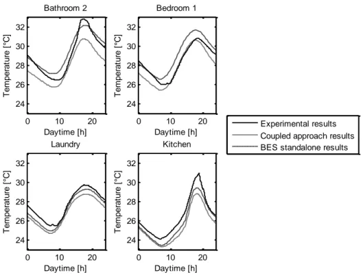
First, Figure 10 illustrates the impact of the coupling approach on the results of small rooms. Generally, the coupling approach decreases the simulated temperature. The coupling approach does not change the shape of the curve, but only translates the results. As demonstrated in the figure, the coupling approach has almost no impact on the parameters of the 10 small rooms. Moreover, these changes are insignificant given the uncertainty range of several parameters, such as U-values of windows. 0 10 20 24 26 28 30 32 Kitchen Te m p e ra tu re [ °C ] Daytime [h] 0 10 20 24 26 28 30 32 Laundry Te m p e ra tu re [ °C ] Daytime [h] 0 10 20 24 26 28 30 32 Bedroom 1 Te m p e ra tu re [ °C ] Daytime [h] 0 10 20 24 26 28 30 32 Bathroom 2 Daytime [h] Te m p e ra tu re [ °C ] Experimental results Coupled approach results BES standalone results

Figure 10: Thermal behaviour of four rooms (coupling approach)

The correlation coefficient, R², and slope coefficient of these results was again evaluated, and the results reproduced in Table 3.

Table 3: Optimisation parameters comparison between BES standalone and coupling approach

Correlation coefficient R² Slope coefficient

BES standalone Coupling approach BES standalone Coupling approach

22

Bathroom 1 0.92 0.92 0.98 0.97

Laundry 0.98 0.98 1.04 1.04

Professional office 0.95 0.95 1.15 1.17

Total 0.94 0.94 0.98 0.98

Because the results remain inside the ASHRAE [26] recommended ranges of values, the coupling approach does not affect the ability of BES to accurately predict the thermal behaviour of small rooms.

7.2 Open space results

Figure 11 illustrates the temperature change measured by sensors 1, 4, 6 and 8 in the open space, which respond to heights of 0.1, 1.9, 3.1 and 4.3 m, respectively.

0 5 10 15 20 22 23 24 25 26 27 28 29 30 Daytime [h] Te m p e ra tu re [ °C ] Numerical results 0.1m high 1.9m high 3.1m high 4.3m high Experimental results 0.1m high 1.9m high 3.1m high 4.3m high

Figure 11: Thermal behaviour of the entrance hall (coupling approach)

The numerical and experimental results are very close. The mean error is -0.01°C (CFD slightly underestimates the measured values), while the absolute mean error is 0.33°C (less than 5% of

23

the temperature range). This mean absolute error is smaller than the measurement error, which underlines the accuracy of the coupling approach.

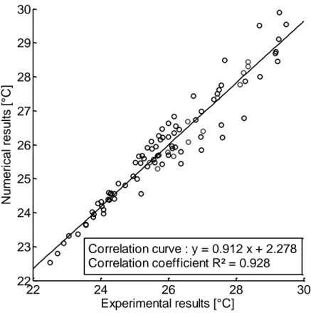
The slope coefficient and correlation coefficient, R², of the CFD results were 0.912 and 0.928, respectively, which is inside the acceptable range defined by ASHRAE [26]. These results are illustrated in Figure 12. 22 24 26 28 30 22 23 24 25 26 27 28 29 30 Experimental results [°C] N u m e ri ca l re su lt s [° C ] Correlation curve : y = 0.912 x + 2.278 Correlation coefficient R² = 0.928

Figure 12: Experimental results versus numerical results

Moreover, the stratification was accurately predicted, because the minimum and maximum temperatures inside the open space were known in the CFD part of the coupling simulation with a precision of 0.05°C and 0.2°C, respectively.

24

Because the maximum temperature of the open space reflects the overheating risks inside the house and was correctly modelled, the objective of this coupling approach was achieved. Finally, the intraday thermal changes were also well described, because the times of minimum and maximum temperature were correctly evaluated.

Due to this accuracy, natural cooling strategies and optimised HVAC devices could be evaluated with this coupling approach to improve the performance of buildings and minimise energy waste in the building sector.

8. Conclusions

To improve the overheating prediction, a coupling BES-CFD approach was developed for multi-storey buildings based on TRNSYS-FLUENT programmes. This paper presents a state-of-the art BES-CFD coupling approach and describes a new coupling scheme. This scheme transfers internal surface temperatures and mass flow from BES to CFD, and CFD supplies heat transfer coefficients and mean temperatures by storey (to consider pressure variations due to

stratification) from CFD to BES. The developed coupling scheme ensures an optimal space and time coupling to optimise the computing time and resources. In the developed tool, BES is in charge of the main part of the effort, while CFD intervenes punctually for one single room (the open space).

The authors have applied this tool to a typical Belgian two-storey house to evaluate

breakthroughs that could be expected with this approach in terms of improving the comfort of occupants during sunny summer days. The results show that BES alone cannot describe the thermal behaviour of the entire building due to known limitations of BES, such as stratification description in high and large vertical development rooms. However, this coupling tool can obtain accurate results everywhere inside the house for an entire sunny day within an acceptable

25

calculation time (4 hours). The stratification of the open space is well described, while the maximum temperature value and time are also precisely known. The coupled tool was validated using measured data, and the mean absolute error was less than 5% of the temperature range, which is smaller than the measurement error.

This new approach can be applied on an entire building to predict the overheating risks and study technical solutions during the design phase of a new construction. Unfortunately, this coupling approach is still complex to implement. Efforts will be necessary to implement automatic coupling based on a BES model. Moreover, this coupling tool requires highly skilled building engineers. Nevertheless, breakthroughs in this approach should guarantee the interest of building engineers and architects because they urgently require improved simulation tools.

Finally, given the actual context of environmental issues, this technique represents an important breakthrough toward naturally cooled buildings and energy-integrated conception. BES-CFD coupling has been proven as an advanced simulation tool that can help to optimise architectural environments by better considering overheating risks to provide more complete and accurate results for thermo-aeraulic phenomena.

Acknowledgments

This research is a part of the SIMBA project. It was supported by the European Regional Development Fund (ERDF) and the Walloon Region.

References

[1] Pérez-Lombarda, L., Ortiz, J. and Pout, C. (2008). A review on buildings energy consumption information. Energy and Build., 40(3), 394-398.

26

[2] Chen, Q. (2009). Ventilation performance prediction for buildings: a method overview and recent applications. Build. and Environ., 44, 848-858.

[3] Schaelin, A., Dorer, V., van der Mass, J. and Moser, A. (1993). Improvement of multizone model predictions by detailed flow path values from CFD calculation. ASHRAE Trans., 93-7-4, 709-720.

[4] Heiselberg, P., Murakami, S. and Roulet, C.-A. (1998) Ventilation of large spaces in buildings: analysis and prediction techniques, International Energy Agency (IEA Annex 26: Energy ventilation of large enclosures), Aalborg University Denmark.

[5] Gao, Y. and Chen, Q. (2003). Coupling a multi-zone airflow analysis program with a computational fluid dynamics program for indoor air quality studies. Proceedings of the 4th International Symposium on HVAC, Vol 1, pp. 236-242 Beijing (China).

[6] Kuznik, F., Rusaouën, G. and Brau, J. (2007) Experimental and numerical study of a full scale ventilated enclosure: Comparison of four two equations closure turbulence models, Build. and Environ., 42, 1043-1053.

[7] Chen, Q., Lee, K., Mazumdar, S., Poussou, S., Wang, L., Wang, M. and Zhang, Z. (2010). Ventilation performance prediction for buildings : Model assessment. Build. and Environ., 45, 295-303.

[8] Barbason, M. and Reiter, S. (2011). A validation process for CFD use in building physics - study of the different scales. Proceedings of ROOMVENT 2011, Trondheim (Norway). [9] Jiang, Y. and Chen, Q. (2003) Buoyancy-driven single-sided natural ventilation in

buildings with large openings, Int. j. of heat and mass transf., 46, 973-988.

[10] Nguyen, A.T. and Reiter, S. (2011) The effect of ceiling configurations on indoor air motion and ventilation flow rates. Build. and Environ., 46, 1211-1222.

27

[11] Yang C., Yang X., Xu Y., and Srebric J. (2007) Contaminant Disperson in personal displacement ventilation. Proceedings of the IBPSA Building Simulation 2007, 818-824. [12] Barbason, M. and Reiter, S. (2011(b)). A validation process for CFD use in building

physics - study of the contaminant dispersion. Proceedings of ACOMEN 2011, Liège (Belgium).

[13] Reiter, S. (2010). Assessing wind comfort in urban planning. Environ. and plan. B: Plan. and des. 37 (5), 857-873.

[14] Ashie, Y. and Kono, T. (2011). Urban-scale CFD analysis in support of a climate-sensitive design for the Tokyo Bay area, Int. j. of climatol., 31, 174-188.

[15] Li, Y. and Nielsen, P. V. (2011) CFD and ventilation research, Indoor Air, 21, 442-453. [16] Rohdin, P. and Moshfegh, B. (2007). Numerical predictions of indoor climate in large

industrial premises. A comparison between different k-ε models supported by field measurements. Build. and Environ., 42 (11) : 3872-82.

[17] Zhai, Z., Zhang, Z., Zhang, W. and Chen, Q. (2007). Evaluation of various turbulence models in predicting airflow and turbulence in enclosed environments by CFD: part 1 – summary of prevalent turbulence models. HVAC&R Res., 13(6), 853-870.

[18] Barbason, M. and Reiter, S. (2010). About the choice of a turbulence model in building physics simulations. Proceedings of the 7th International Conference on Indoor Air Quality, Ventilation and Energy Conservation in Buildings (IAQVEC 2010), Syracuse (New York). [19] Zhai, Z., Chen, Q., Haves, P. and Klems, J. H. (2002) On approaches to couple energy

simulation and computational fluid dynamics programs, Build. and Environ., 37, 857-864. [20] Negrão, C. (1995) Conflation of computational fluid dynamics and building thermal

28

[21] Zhai, Z. and Chen, Q. (2003) Solution characters of iterative coupling between energy simulation and CFD programs, Energy and Build., 35, 493-505.

[22] Wang, L. and Chen, Q. (2007) Theoretical and numerical studies of coupling multizone and CFD models for building air distribution simulations, Indoor Air, 17 348-361.

[23] Wang, L. (2007) Coupling of multizone and CFD programs for building airflow and contaminant transport simulations. PhD Thesis, Purdue University US-IN.

[24] Djunaedy, E., Hensen, J. L. M. and Loomans, M. G. L. C. (2005) External coupling between CFD and energy simulation: implementation and validation, ASHRAE Trans., 111, 612-624.

[25] Pappas, A. and Zhai, Z. (2008). Numerical investigation on thermal performance and correlations of double skin façade with buoyancy-driven airflow. Energy and Build., 40, 466-475.

[26] ASHRAE (2009) ASHRAE handbook of Fundamentals. ASHRAE, Atlanta, GA.

[27] Nielsen, P. V., Allard, F., Awbi, H. B., Davidson, L., and Schaelin, A. (2007) Computational Fluid Dynamics in Ventilation Design. REHVA guideb. 10.

[28] Cook, M. J. and Lomas, K. J. (1997) Guidance on the use of computational fluid dynamics for modelling buoyancy-driven-flows, Proceedings of the IBPSA Building Simulation Conference, Prague (Czech Republich).

[29] Solar Energy Laboratory (2010) TRNSYS User Manual (Version 17.00.0013).

[30] Crawley, D. B., Hand, J. W., Kummert, M. and Griffith, B. T. (2008) Contrasting the capabilities of building energy performance simulation programs. Build. and Environ., 43, 661-673.