Constrained Trajectory Optimization of a Soft Lunar
Landing from a Parking Orbit
by
Alisa Michelle Hawkins
B.S., Georgia Institute of Technology (2003)
Submitted to the Department of Aeronautics and Astronautics in partial fulfillment of the requirements for the degree of
Master of Science in Aeronautics and Astronautics at the
MASSACHUSETTS INSTITUTE OF TECHNOLOGY June 2005
©
Alisa Michelle Hawkins, 2005. All rights reserved.The author hereby grants to MIT permission to reproduce and distribute publicly paper and electronic copies of this thesis document in whole or in part.
Author: 4 V~~-- .
Department of Aeronautics and Astronautics May 20, 2005
C ertified by: T J i
)Thomas J. Fill Principle Member of the Technical Staff, Draper Laboratory Thesis Supervisor
/1) Certified by:
(Ronald Jfroulx Principle Member of the Technical Staff, Draper Laboratory
Thesis Supervisor
Certified by:
Associate Professor of Aeronautics
Accepted by
MASSACHUSETTS INS E OF TECHNOLOGY
[JUN
2 3 2005
Eric M. Feron and Astronautics, M.I.T. pTesis Supervisor
I' H ~t
Jaime Peraire Professor of Aerbnia tics and Astronautics, M.I.T. Chair, Committee on Graduate Students
Constrained Trajectory Optimization of a Soft Lunar Landing
from a Parking Orbit
by
Alisa Michelle Hawkins
Submitted to the Department of Aeronautics and Astronautics on May 20, 2005, in partial fulfillment of the
requirements for the degree of
Master of Science in Aeronautics and Astronautics
Abstract
A trajectory optimization study for a soft landing on the Moon, which analyzed the effects of adding operationally based constraints on the behavior of the minimum fuel trajectory, has been completed. Metrics of trajectory evaluation included fuel expenditure, terminal attitude, thrust histories, etc.. The vehicle was initialized in a circular parking orbit and the trajectory divided into three distinct phases: de-orbit, descent, and braking. Analy-sis was initially performed with two-dimensional translational motion, and the minimally constrained optimal trajectory was found to be operationally infeasible. Operational con-straints, such as a positive descent orbit perilune height and a vertical terminal velocity, were imposed to obtain a viable trajectory, but the final vehicle attitude and landing ap-proach angle remained largely horizontal. This motivated inclusion of attitude kinematics and constraints to the system. With rotational motion included, the optimal solution was feasible, but the trajectory still had undesirable characteristics. Constraining the throttle to maximum during braking produced a steeper approach, but used the most fuel. The results suggested a terminal vertical descent was a desirable fourth segment of the tra-jectory, which was imposed by first flying to an offset point and then enforcing a vertical descent, and provided extra safely margin prior to landing. In this research, the relative effects of adding operational constraints were documented and can be used as a baseline study for further detailed trajectory optimization.
Thesis Supervisor: Thomas J. Fill
Title: Principle Member of the Technical Staff, Draper Laboratory
Thesis Supervisor: Ronald J. Proulx
Title: Principle Member of the Technical Staff, Draper Laboratory
Thesis Supervisor: Eric M. Feron
Acknowledgments
During my time at MIT and Draper Laboratory, I have worked with some amazing people who have helped me grow, on both intellectual and personal levels. This work would not
have been possible if not for the guidance and support of Thomas Fill and Ronald Proulx, who gave freely of their time to support this research. Tom, thank you for your never-ending support, patience, attention to detail, and amazing wealth of knowledge. I have learned a great deal from you, which I hope to carry with me in my professional career. Ron, thank you for your vision and for always pushing the project forward. I admire your passion and dedication. Much gratitude is given to Eric Feron for being a constant source of enthusiasm and for having a desire to think out-of-the-box. I also would like to thank David Geller, Michael Luniewicz, Linda Fuhrman, and Lee Norris whom I had the pleasure of working with for brief periods of time, and Michael Ross for providing insight into your DIDO package. Special thanks to Anil Rao and Peter Neirinckx for checking in on me from time to time. I would also like to thank the Draper library staff for ordering an endless stream of literature for me. Rachel, thanks for being a great officemate. And special thanks to the roommates of 268 Broadway: Geoff, Megan, and Steve. Above all, I would like to thank my family, who's love and support has gotten me to where I am today. And to No8l, my love, thank you for everything. This adventure would not have been complete without you. Thank you for sharing this experience with me.
This thesis is dedicated to my grandparents:
Roland P. and Odette M. Jotterand & Joseph F. and Sophronia V. Hawkins, Sr.
This thesis was prepared at the Charles Stark Draper Laboratory, Inc., under Internal Research and Development Project 12601-001, GCDLF Support.
Publication of this thesis does not constitute approval by Draper or the sponsoring agency of the findings or conclusions contained herein. It is published for the exchange and stimulation of ideas.
Contents
1 Introduction 15
1.1 Review of Previous Work . . . 16
1.2 Thesis Overview. . . . 18
1.3 Nomenclature . . . 20
2 Optimization Background 21 2.1 Basic Optimization . . . 21
2.1.1 Finding a Minimum . . . 23
2.1.2 Equality Constrained Optimization . . . . 23
2.1.3 Inequality Constrained Optimization . . . 24
2.1.4 Optimal Control . . . 25
2.1.5 Pontryagin's Minimum Principle . . . 27
2.2 Numerical Methods . . . 28
2.2.1 Direct Methods . . . 28
2.2.2 Direct Transcription Methods using Spectral Techniques . . . 29
2.2.3 Implementation . . . . 30
3 Moon Landing Problem 41 3.1 Assumptions . . . 41
3.2 Reference Frames and Coordinate Systems . . . 42
3.3 Orbital Dynamics Definitions . . . 44
3.4 Angle Definitions . . . 45
3.6 Operational Considerations Included in the Optimization Design Problem 3.7 Vehicle Specifications . . . .
4 Equations of Motion
4.1 Six Degree-of-Freedom EOM . . . . 4.1.1 Translational Dynamics . . . .
4.1.2 Rotational Dynamics . . . . 4.1.3 Mass Flow Equation . . . . 4.2 Planar Equations of Motion . . . . 4.2.1 Translational Dynamics in Cartesian Form 4.2.2 Translational Dynamics in Polar Form . . 4.2.3 Rotational Kinematics . . . . 4.2.4 Variable Mass . . . . 53 . . . 5 3 . . . 5 3 . . . 54 . . . 5 6 . . . 5 6 . . . . 5 7 . . . 5 7 . . . 5 8 . . . 5 8 5 Results 5.1 Translational Motion (TM) . . . . 5.1.1 Baseline Trajectory (TM) . . . . 5.1.2 Baseline Trajectory with Knots (TM) . . . . 5.1.3 Inclusion of Selected Operational Constraints (TM) . . . . 5.2 Translational Motion with Rotation (TMR) . . . . 5.2.1 Constrained Optimal Trajectory with Rotational Motion (TMR) . 5.2.2 Descent Orbit Perilune Height Study (TMR) . . . . 5.2.3 Terminal Vertical Descent Study (TMR) . . . .
6 Conclusion
6.1 Summary of Analysis . . . . 6.2 Significant Findings . . . . 6.3 Recommendations of Future Work . . . .
8 49 50 59 60 62 74 82 98 102 114 124 135 135 136 138
List of Figures
2-1 2-2 2-3 2-4 2-5 2-6 2-7 2-8 3-1 3-2 3-3 3-4 3-5 3-6 3-7 5-1 5-2 5-3 5-4 5-5 5-6 5-7 . . . . 22 . . . . 30 . . . . 30 . . . . 34 . . . . 35 . . . . 36 . . . . 37 . . . . 38 One-dimensional Convexity . . . . Legendre-Gauss-Lobatto Points . . . . Vertical Descent Diagram . . . . Vertical Descent Minimum Fuel Solution (Normalized Units) . .DIDO Estimated Hamiltonian and Costate (Normalized Units) .
Estimated Switching Function . . . . K not Inclusion . . . .
Vertical Descent Solution With One Knot (Normalized Units)
Three-Dimensional Inertial and Body Reference Frames . . . . . Two-Dimensional Inertial and Body Reference Frames . . . . Two-Dimensional Inertial and Rotating Polar Frames . . . . Orbital Dynamics Definitions . . . .
Thrust Angle Definitions . . . . Angle Definitions . . . . Position of Circular Orbit Case . . . .
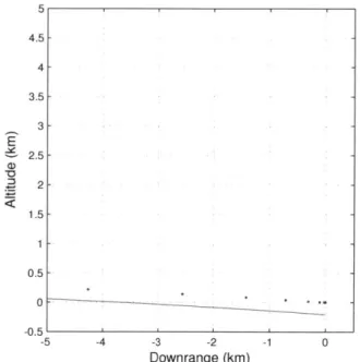
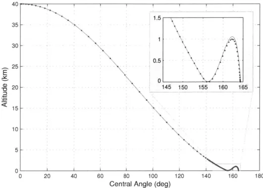
Baseline Trajectory Profile (TM) . . . . Baseline Altitude vs. Range during Final Braking Phase . . . .
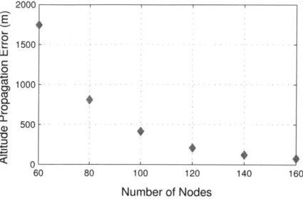
Baseline Altitude vs. Range (Equally Scaled Axes) . . . . Final Propagation Error in Altitude . . . .
Baseline Trajectory Results (TM) . . . .
Baseline Trajectory Results (TM) . . . . Baseline Trajectory Results (Starting from 1.5 km) (TM) . . . .
64 64 65 66 67 68 69 42 43 43 44 45 46 48
5-8 Baseline Trajectory Results (Starting from 1.5 km) (TM) . . . . 70
5-9 Baseline Trajectory Hamiltonian and Costate Components . . . 73
5-10 Baseline Trajectory Profile with Knots (TM) . . . 75
5-11 Baseline Trajectory Results with Knots (TM) . . . 77
5-12 Baseline Trajectory Results with Knots (TM) . . . 78
5-13 Baseline Trajectory Results with Knots (Starting from 1.5 km) (TM) . . . 79
5-14 Baseline Trajectory Results with Knots (Starting from 1.5 km) (TM) . . . 80
5-15 Throttle Bounds and Number of Nodes for Open Throttle Cases . . . 84
5-16 Open Throttle DOPH Parametric Study (TM), Dashed lines represent in-crem ents of 5 km . . . 85
5-17 Throttle Profile (20 km Target Perilune Height) . . . 85
5-18 Throttle Profile (-10 km Target Perilune Height) . . . 87
5-19 Throttle Bounds for Continuous Thrust Cases . . . 87
5-20 Continuous Thrust DOPH Parametric Study (TM), Dashed lines represent increments of 5 km (TM) . . . 89
5-21 Continuous Thrust (TM), Left Plot: Altitude vs. Downrange (Equally Scaled Axes), Right Plot: Thrust Direction Angle during Braking Phase . 90 5-22 Throttle Comparison for 20 km Target Perilune Height Cases . . . 91
5-23 DOPH Parametric Study AV Results (TM) . . . 91
5-24 DOPH Parametric Study Fuel Usage Results (TM) . . . 92
5-25 Lofting Suppression Result for -10 km Case (TM) . . . 94
5-26 Parametric Study Fuel Usage Results (TM) . . . 97
5-27 Weighted Minimum Fuel Local Optimum Trajectory Profile; +15 km DOPH (T M R ) . . . 105
5-28 TMR +15 km DOPH, Altitude vs. Downrange during Final Braking Phase 106 5-29 TMR +15 km DOPH, Altitude vs. Downrange (Equally Scaled Axes) . . 106
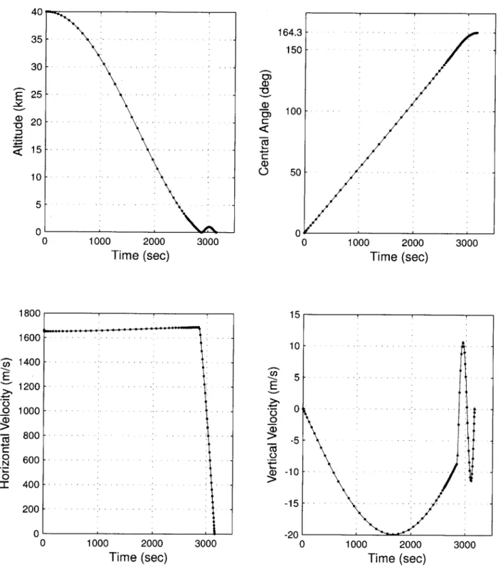
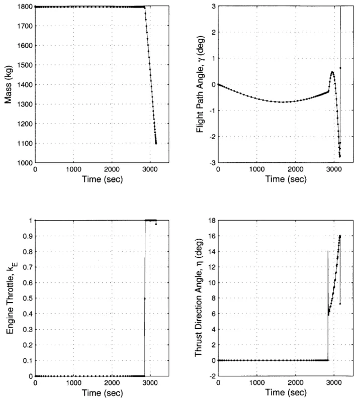
5-30 TMR +15 km Targeted Perilune Trajectory Results . . . 107
5-31 TMR +15 km Targeted Perilune Trajectory Results . . . 108
5-32 TMR +15 km Targeted Perilune Case, Angular Rate and Acceleration . . 109
5-33 TMR +15 km Targeted Perilune Trajectory Results (Braking Phase) . . . 110
5-34 TMR +15 km Targeted Perilune Trajectory Results (Braking Phase) . . . 111 5-35 TMR +15 km Targeted Perilune Case, Angular Rate and Acceleration
(Braking Phase) (TM R) . . . 112 5-36 Continuous Thrust with Attitude Constraints . . . 116 5-37 Continuous Thrust (TMR), Altitude vs. Downrange during Braking Phase 116 5-38 Continuous Thrust (TMR), Altitude vs. Downrange (Equally Scaled Axes) 117 5-39 Continuous Thrust (TMR), Throttle and Thrust Direction Angle Profiles
(Braking Phase) . . . 118 5-40 Maximum Thrust with Attitude Constraints . . . 120 5-41 Maximum Thrust (TMR), Altitude vs. Downrange during Braking Phase . 120 5-42 Maximum Thrust (TMR), Left Plot: Altitude vs. Downrange (Equally
Scaled Axes), Right Plot: Thrust Direction Angle during Braking Phase. . 121 5-43 TMR Parametric Study AV Results and Comparison to TM Data . . . 122 5-44 TMR Parametric Study Fuel Results and Comparison to TM Data . . . 123 5-45 Vertical Descent Constraints . . . 126 5-46 Vertical Descent Study AV Requirements (TMR) . . . 128 5-47 Vertical Descent Study Fuel Usage (TMR) . . . 128 5-48 Altitude vs. Downrange (during Final Braking Phase) for Cases Targeting
2 km Offset Altitude, (TMR) . . . 132 5-49 Zoomed Altitude vs. Downrange for Cases Targeting 2 km Offset Altitude
(T M R ) . . . 132 5-50 Throttle and Thrust Direction Angle, Case N and V (TMR) . . . 133 5-51 Throttle and Thrust Direction Angle, Case A and AV (TMR) . . . 134
List of Tables
2.1 Vertical Descent Parameter Values . . . . 32
5.1 Initial Conditions and Vehicle Parameters . . . . 62
5.2 Open Throttle during De-orbit and Braking Phases, Tabulated Data A . . 86
5.3 Open Throttle during De-orbit and Braking Phases, Tabulated Data B . . 86
5.4 Continuous Thrust Case, Tabulated Data . . . . 90
5.5 Addition of Non-zero Terminal Velocity Constraint to Continuous Thrust Case, Tabulated Data . . . . 95
5.6 Comparison of Scaled Values . . . 101
5.7 Continuous Thrust with Attitude Constraints, Tabulated Data . . . 119
5.8 Maximum Thrust with Attitude Constraints, Tabulated Data . . . 121
5.9 Fuel and AV Usages for Vertical Descent Study . . . 129
Chapter 1
Introduction
Trajectory design is a crucial process during the planning phase of a spacecraft landing mission. The trajectory must meet all mission objectives, while complying with vehicle limitations and capabilities. The common approach to designing a spacecraft landing trajectory is to first focus on the translational motion, while treating the vehicle as a point mass. Trajectory planners concentrate on the overall shape of the trajectory before attitude dynamics are considered. Once a trajectory is determined, guidance algorithms are created to guide the vehicle along the given trajectory. Because fuel mass is a major driver of the total vehicle mass, and thus mission cost, the objective of most guidance algorithms is to minimize the required fuel consumption. Most of the existing algorithms are termed as "near-optimal" in terms of fuel expenditure.
The question arises as to how close to optimal are these guidance algorithms. To answer this question, numerical trajectory optimization techniques are often required. One such technique is applied in the current research to find these minimum fuel opti-mal trajectories. In most cases, attitude dynamics are not considered in exploring these "minimum fuel" trajectories. The contribution of this thesis is to included attitude dy-namics in the optimization problem and assess the effect of these dydy-namics on the optimal trajectory.
Recently, renewed interest in returning to the lunar surface has been expressed. The "The Vision for Space Exploration", NASA, February 2004, http://www.nasa.gov/missions/solarsystem/explore-main.html
Moon has been proposed as a base for extended missions. During a landing on the Moon, there is no atmospheric drag to slow the vehicle from orbital velocities to near-zero at the surface. Instead, an onboard propulsion system is required for this purpose. The vehicle must be capable of sensing the surface and landing at an attitude which places all landing gears simultaneously and squarely on the ground. This thesis considers the optimal fuel requirements to efficiently satisfy the trajectory and attitude requirements simultaneously in the landing problem.
1.1
Review of Previous Work
Previous work that relates to the current research falls into the two categories of guidance algorithms and trajectory optimization for lunar landings. A guidance algorithm is used to fly the vehicle during the actual mission. Trajectory optimization techniques are used to verify that the guidance algorithms produce the most efficient or near-efficient trajectories for the vehicle to follow. Previous work performed in these areas are presented next.
The race for the Moon in the 1960's generated a large impetus for the research and development of guidance algorithms for the soft landing of vehicles on the lunar surface. The majority of lunar landing research was performed during the Apollo era in the 1960's. Studies were performed to develop guidance algorithms, descent trajectories, transfer orbit properties, etc.. These studies included a detailed parametric study by Akridge and Harlin [1], who varied parameters such as initial parking orbit altitudes, thrust-to-weight ratio, and the specific impulse of the engine. A study of lunar landing orbits was performed by Cavoti [2] for both range-free and range-fixed problems, with the assumption of a two impulse burn. This study theoretically showed that the minimum-fuel descent transfer orbit could not be an exact Hohmann type orbit (tangential thrusting at apolune and perilune) and meet the terminal vertical attitude constraints. Cavoti found that the solution was to burn at a slight angle to the tangential direction. Trajectory analysis work, done by Bennett and Price [3], was the basis for dividing the powered descent phase of the Apollo landing trajectory into three phases: an fuel-optimum braking phase, a landing approach transition phase, and a terminal descent phase.
Existing guidance algorithms, which were vigorously tested, landed five Surveyor vehi-cles and six Apollo lunar modules successfully on the surface of the Moon. The Surveyor vehicles used a guidance scheme based on the work done by Cheng and Pfeffer [4], which controlled the velocity and slant range of the vehicle during the final descent. The attitude control law used is known as a "gravity turn" [5], which tended to force the flight path towards the vertical as time progressed. The Apollo missions used an explicit guidance algorithm, which was originally derived by Cherry [6] and then simplified by Klumpp [7] to be used onboard the lunar module guidance computer.
Several other guidance algorithms were proposed during the same time period. A proportional navigational guidance algorithm was proposed by Hall, Dietrich, and Tiernan [8], which was modified from work done by Kriegsman and Reiss [9]. More recently (in 1999), a near-minimum fuel law was proposed by Ueno and Yamaguchi [10].
Most of the aforementioned guidance algorithms were designed to minimize fuel, while minding safety and operational considerations. Optimality, or near-optimality, can only be proven for some of these algorithms given certain assumptions, such as constant thrust or constant gravity. To prove optimality, trajectory optimization and optimal control theory must be used. Trajectory optimization capabilities during the Apollo era were severely limited by computing power. An analytic solution for the one-dimensional vertical terminal descent of a lunar soft-landing, based on an application of Pontryagin's minimum principle, was found by Meditch [11] in 1964. Meditch showed the existence of an optimum thrust program that achieves soft landing under powered descent, which includes the real-time calculation of a switching function as the vehicle descends to the surface. Extensive numerical research on the one-dimensional problem was performed by Teng and Kumar [12], using various cost functionals. Their method is based on a time transformation, applied to the calculus of variations. The solution was found numerically, using a quasi-linearization method. In 1971, Shi and Eckstein [13] derived an exact analytic solution for the problem which Teng and Kumar addressed.
With the increase in computing power, trajectory optimization techniques, of the type to be discussed in Section 2.2, have greatly increased the feasibility of generating optimal trajectories with higher complexity and applicability. Recently, Vasile and Floberghagen
[14] applied a Spectral Elements in Time (SET) approach to the lunar soft-landing prob-lem. Within the work, a lunar landing descent from three parking orbit scenarios down to an altitude of 2 m above the surface was optimized. The cost function used was based on the square of the control input, which has been noted to be different from the minimum fuel solution [15] used in the current research. In the section to follow, the approach for the trajectory optimization followed in the current research is outlined.
1.2
Thesis Overview
This thesis investigates the problem of soft-landing a vehicle on the surface of the Moon from an initial circular parking orbit, using a trajectory optimization technique. The objectives of the current research are to:
1. Determine operationally feasible landing trajectories, which minimize fuel expendi-ture, while considering the finite rotational motion of the vehicle and operational attitude constraints.
2. Analyze the fuel usage penalties and trajectory performance effects due to the in-clusion of each operational constraint considered. Metrics of trajectory performance include terminal attitude, terminal velocity, control histories, steepness of approach to the landing site, etc..
The optimization method used to explore the Moon landing problem in the current research is the Legendre Pseudospectral Method. The Legendre Pseudospectral Method has been applied to a variety of trajectory optimization problems, including problems of ascent guidance [16], satellite formation flying [17], and impulsive orbit transfers [18]. DIDO [19] is used to implement the Legendre Pseudospectral Method in the current research. The entire trajectory, from de-orbit to soft landing, is included in the analysis and is treated as a single problem. This is done in order to generate a trajectory which is optimal over the entire time span of the landing process.
In considering both translational and rotational motion in the trajectory optimization of a soft-landing on the Moon, a direct comparison is made between results that include
rotational motion and those that do not, to gain insight into the effect on the fuel usage. The inclusion of the attitude dynamics in the optimization framework to see how the trajectory is reshaped by the attitude constraints is a major contribution of the current research. An outline of the thesis is given below.
First, an overview of basic optimization theory is given in Chapter 2, along with the numerical methods currently used in solving optimal control problems. The numerical method used in the current research, the Legendre Pseudospectral Method, is discussed
and a simple example is presented to explain the implementation of the method.
Chapter 3 outlines the specifics of the landing problem. The coordinate frames used, and assumptions made, are discussed. An overview of the trajectory is given, as well as the assumed vehicle parameters. Operational requirements for a successful landing on the lunar surface are discussed.
The equations of motion are derived in Chapter 4. Full six degree-of-freedom (DOF) equations of motion (EOM) are derived in cartesian coordinates. Vehicle motion is as-sumed to be planar in the current research (though it can easily be extended to three dimensions) and the 6DOF EOM are reduced to this simplified case. The planar EOM are implemented in the optimization code.
The results obtained from trajectory optimization of the Moon Landing problem are presented in Chapter 5. A baseline trajectory is presented first, before progressing to more constrained scenarios (based on operational considerations). Results obtained for two-dimensional translational motion (TM) are explored first. Selected operational con-siderations related to the perilune height of the descent orbit, continuous thrusting, and a near-zero terminal velocity are implemented. The effects of these constraints on the trajectory are investigated. Next, the attitude dynamics are added to the optimization framework. Finally, a vertical descent phase is added to the trajectory and analyzed. The significant findings and a conclusion are given in Chapter 6, as well as avenues of future work.
1.3
Nomenclature
Standard nomenclature, defined below for an arbitrary variable (x), has been used through-out this document.
1.
{x}:
Regular characters represent scalar quantities or magnitudes of the correspond-ing vector.2.
{x}:
Bold, lower case characters represent vectors.3.
{X}:
Bold, upper case characters represent matrices.4.
{±}:
Overhead dots represent the time derivative of the variable.5.
{x',
xb, xr}: Superscripts denote the reference frame in which a vector is defined, where i, b, and r represent inertial, body, and rotating frames, respectively.Chapter 2
Optimization Background
The objective of this chapter is to highlight key concepts necessary to understand the optimization analysis performed in subscquent chapters. The reader is referred to the following references for in depth coverage of the corresponding fields: Nonlinear pro-gramming ([20]), Optimal Control Theory ([21], [22]), and the Legendre Pseudospectral Method
([23]).
A summary of trajectory optimization as a whole, including the first two topics mentioned above, is given by Betts [24].The first section in this chapter is an overview of optimization theory, while the second describes numerical methods used for solving optimal control problems.
2.1
Basic Optimization
An optimization problem is any problem where it is desired to maximize (or minimize) a specified criterion. This criterion is referred to as a cost function, which is a function of the parameters over which the optimization takes place.
Let x E R' be a vector of parameters and let J(x) : R' -+ R define a cost function. It is desired to find the value x* which minimizes J out of all admissible x. The global minimum is defined as:
Nnnvex, f f Global Global Optimum
t
Optimum Local Optimum - I - I x* x x* xFigure 2-1: One-dimensional Convexity
A local minimum is defined as:
J(x*) < J(x) for all x in the neighborhood of x* (2.2)
If a function is globally convex (it monotonically increases in every direction from
the global optimum), then any local optimum found is also the global optimum. If the function is nonconvex, finding a local optimum does not necessarily imply that it is also the global optimum solution. The concept of convexity vs. nonconvexity and local vs. global optimums for an arbitrary one-dimensional function f(x) is illustrated in Figure 2-1.
In the convex example, only one optimal solution exists, which is the global optimum. In the nonconvex example, two optimal solutions exist. One is a local optimum, while the other is the global optimum. Most trajectory optimization problems are nonconvex and therefore only local optimums are readily found.
A parameter optimization problem that has a linear cost function, linear constraints,
and has only real values is known as a linear programming problem. The term is only used for problems which have real values, otherwise it falls into the category of integer or mixed-integer programming. If the problem has only real values, but includes a nonlinear cost function or nonlinear constraints, it is referred to as a nonlinear programming (NLP) problem.
22 Connvx
2.1.1
Finding a Minimum
From basic calculus, recall that a local minimum of a function, which is the function of one variable (i.e., f(x)), can be found by locating a point where the first derivative of the function with respect to the variable equals zero and the second derivative is positive.
This notion is expanded to higher dimensions with gradients and Hessians. A gradient is a vector consisting of the first-order partial derivatives of a function with respect to each variable. The Hessian is a matrix consisting of the second-order partial derivatives of the function. For example, the following conditions are satisfied at a local minimum for the cost function J(x):
0 (2.3)
-09
ax
02j
J>
0 (2.4)jx2
-One could attempt to determine the minimum of the cost function analytically, but it may be difficult or impossible. Therefore, iterative techniques are used to locate the minimum by searching over the region of admissible x. Newton's method, the most common technique, uses the gradient and Hessian information at the current location to determine a search direction. There are numerous other iterative techniques used, most being based on the principle of Newton's method.
2.1.2
Equality Constrained Optimization
Equality constraints are added to the optimization problem if it is desired that a function, or functions, of the parameters equal a specific value. The parameters can vary, but relationships between the parameters remain fixed. An equality constraint has the form:
f(x) = 0 (2.5)
where f : R" --> R.
is to formulate the augmented cost function, which is a combination of the cost function and the constraints with multipliers.
J' = J(x) + A'f(x) (2.6)
To find the minimum, the gradient of J' is taken with respect to x and A and set to zero. The first-order necessary conditions for optimality become:
a
= + OA 0 (2.7) ax Ox 9x = f(x) = 0 (2.8) BA2.1.3
Inequality Constrained Optimization
In addition to equality constraints, some problems have inequality constraints. An in-equality constraint has the form:
g(x) < 0 (2.9)
where g : R" - RP.
The constraints are adjoined to the cost function in a similar manner as the equality constraints, but with the multipliers i. The augmented cost function is now defined as follows:
J= J(x) + ATf (x) + Jig(x) (2.10)
There are two classes of inequality constraints that must be dealt with: active and inactive. The vector g(x) can be written as seen in Equation (2.11), with gi(x) for
(i = 1.. .p) representing individual components of the p-dimensional vector. An active constraint is when a component of the constraint vector equals zero at the optimum solution, (i.e., gi(x*) = 0). The optimization problem is bounded by these constraints. Inactive constraints are constraints where gi(x*) < 0 and these constraints do not affect the optimal solution. The equation pTg = 0, which is known as complementary slackness, ensures that the individual inequality constraints are either active or do not affect the solution.
Sgi(x)
g =(2.11)
gp (x)
The first-order necessary optimality conditions, also known as the Karush-Kuhn-Tucker (KKT) conditions, are given by Equations (2.8) and (2.9), and the following:
V= 0 (2.12)
;> 0 (2.13)
PiTg = 0 (2.14)
2.1.4 Optimal Control
A special class of optimization problems which include dynamical constraints that vary with time are known as functional optimization problems, where the term "functional" is used to denote a function of a function. Functional optimization problems that have an input, or control, to be determined are known as an optimal control problems. Optimal control problems have a wide variety of applications, including the field of trajectory optimization.
Let x(t) E R' be the state of a continuous system where t E R is time. Furthermore, let u(t) E R"' be the control or input. Lastly, let the dynamical constraints that govern the change of x(t) with respect to time be given as:
x = f (x(t), u(t), t) (2.15)
where f : R" x R1I x R -+ R1.
The general optimal control problem is to find the function u(t) that minimize the cost functional, J, subject to the constraints imposed on the problem (which include the dynamical constraints). It is normally desired to either minimize a functional of the state and control over the entire time span or the final value of a criterion. The cost functional is therefore composed of two parts: a terminal cost
#
: R' x R -- R (commonly referred toas the Mayer cost) and an integrated cost L : R' x R' x R -* R (known as the Lagrange cost). The Bolza form of the cost functional, as seen in Equation (2.16), is a combination of the terminal and integrated costs.
= (x(t), tf) + i (x(t),u(t),t) dt (2.16)
The initial and final boundary conditions that the system must satisfy are given by Equations (2.17) and (2.18), respectively.
0(x(to) to) = 0 (2.17)
Of(x(tf), tf) = 0 (2.18)
where #io: R' x R--+ R0 and :R" xR ---+R
In order to combine all of this information, the augmented cost functional, ', is formulated. The dynamical and terminal constraints are adjoined to the cost functional with a vector of Lagrange multipliers (also known as the costate), A(t)
C R',
and the terminal constraint multipliers, v E R4/. The equation given below is similar to Equation(2.3.5) in Reference [22].
= # (X(tf), tf) + VTO (x(tf), tf)
tf
+ [L (x(t), u(t), t) + A(t)T{f (x(t), u(t), t) -:] dt (2.19)
to
To simplify the augmented cost functional, the Hamiltonian and end point functionals are defined in Equations (2.20) and (2.21), respectively. J' is simplified to Equation (2.22). The functional dependencies have been omitted for clarity.
'H = L + ATf (2.20)
to(2.21)
tft H TS]dt (2.22)
Calculus of variations is used to determine a stationary point of the augmented cost functional. Using the same concepts as before, the variation of J' is taken and appropriate functions are set to zero. The resulting necessary conditions for a local minimum for the free final time problem are derived by Hull [21] as:
ON x f(x,u,t) (2.23) A = -(2.24) Ox 0 = (2.25) Ou o(x(to), to) 0 (2.26) Of(x(tf), tf) = 0 (2.27) AT (tt (2.28) ()tt_ = Ot) (2.29) f t =
These necessary conditions are used later in the thesis to analyze optimality of obtained solutions. Additional optimality conditions, similar to those in Equations (2.13) and (2.14), must be included if there are inequality constraints involved. Additional equality constraints take the same form as that seen in Section 2.1.2.
2.1.5
Pontryagin's Minimum Principle
Equation (2.25) is used to solve directly for the control function u. In some cases (e.g.,
N is a linear function of u), Equation (2.25) is not a function of u and the above method cannot be used to determine the control. Instead, the control is determined with Pontrya-gin's minimum principle [25], which is a more general form of the necessary optimality conditions. Pontryagin's minimum principle can be written as follows:
u* =arg min N (u, x*, A*, t) (2.30)
uEU
general idea is to find the control which minimizes the Hamiltonian at each point along the trajectory.
2.2
Numerical Methods
The previous section outlined optimality conditions, which are to be solved to find a stationary point. For most non-linear optimal control problems, solving these equations analytically is very tedious, or impossible. Researchers have instead turned to numerical methods and computers to aide in finding the optimal solution.
There are numerous numerical methods that have been formulated to solve optimal control problems and it is not in the scope of this thesis to explore them all. The method used in this research is the Legendre Pseudospectral Method, which is a direct transcrip-tion method that uses a spectral technique. The meanings of "direct", "transcriptranscrip-tion",
and "spectral" will be discussed below and an example will be given to explain imple-mentation of this method.
2.2.1
Direct Methods
Numerical methods used in solving optimal control problems fall into two distinct cat-egories: direct and indirect. An indirect method uses information from the costate dif-ferential equations (2.24), the maximum principle (2.30), and the boundary conditions (2.26) - (2.29), to find the optimal solution. In order to use this method an estimate of the costate is required a priori, which may pose a problem since the costate does not usually have physical significance.
The more common approach is to use a direct method, which aims at directly opti-mizing the cost function, Equation (2.16). The method starts from an initial guess of the state and control and searches in the feasible region for a minimum of the cost function. This is reported as a local minimum solution, because it is impossible to search the entire feasible region. If it can be proven that the problem is convex, then local optimality implies global optimality.
Assuming that the user is familiar with the dynamics of the problem being posed, it 28
is much easier to provide an initial guess of the state and control rather than the costate. In some cases, a simple propagation of the state from the desired initial conditions with no control input is sufficient. However, if the problem is highly nonconvex, a good initial guess may be crucial in finding the correct local optimal solution.
A direct method was selected for this research for it simplicity and because it does not require costate estimates a priori. Multiple iterations of the solutions were performed, each time providing the optimizer with a different initial guess of the state and control time histories, in order to provide confidence that the obtained results were in fact the global minimum.
2.2.2
Direct Transcription Methods using Spectral Techniques
Within the class of direct methods, there are distinct categories, including direct shooting methods, direct transcription, etc. A direct transcription method is used in this thesis and will be outlined below.
Most real-time optimal control problems are in the continuous time domain. In order to be implemented on a computer, this continuous time domain system must be transformed into a discrete time domain system. The locations in time at which the problem is discretized are referred to as "nodes", and can be uniformly or non-uniformly distributed in the time domain. At each node, the discrete system represents the continuous system, and links must be made between the nodes to represent the dynamics of the original continuous system. A transcription method is used to transform the continuous system into the discrete problem. Most optimal control problems include either a nonlinear cost function or nonlinear constraints (which may include nonlinear dynamical constraints), that are only functions of real variables. As a result, the transcribed problem is an NLP. The key to a transcription method is not only transforming the problem from a con-tinuous system to a discrete system, but also linking the nodes together in a way that represents the dynamics of the original problem. The dynamics of the continuous system can be represented in several ways within the discrete framework, including the use of the Euler method, the Runge-Kutta method, and spectral methods. The method used in this thesis is a spectral method, which fits globally orthogonal polynomials to the discrete
60 ~,50 0 Z 40 ID30 E Z 20 o10. 0 0 0.2 0.4 0.6 0.8 1
Normalized Time Scale
Figure 2-2: Legendre-Gauss-Lobatto Points
y T
yo- m
9
0'
Figure 2-3: Vertical Descent Diagram
data over the entire time span.
The Legendre Pseudospectral Method uses a special class of orthogonal polynomials, known as Legendre Polynomials. The interior nodes are placed at the roots of the Legen-dre polynomial derivative, known as the LegenLegen-dre-Gauss-Lobatto (LGL) points, which provides higher accuracy in the results. Figure 2-2 shows the placement of the LGL points for cases with 10, 30, and 50 nodes, respectively.
2.2.3
Implementation
DIDO [19] is the software package used to employ the Legendre Pseudospectral Method in the current research. It is easy to use and is capable of solving a wide variety of problems. To explain some of the implementation concepts of DIDO, a simple example is used.
Assume that a vehicle performs a controlled descent from an initial altitude to the surface of the Moon, as seen in Figure 2-3. For simplicity, assume a constant gravity,
g, and a constant engine exhaust velocity, Vex. If the thrust, T, is represented by a throttle command (k
c
[0, 1]) multiplied by a maximum thrust limit, Tmax, the equations of motion are as follows:yz=v
(2.31)Tma k
i = max. -g (2.32)
u=
- Tmaxk (2.33)Vex
where y, v, and m represent the altitude, velocity, and mass respectively.
A minimum fuel solution is desired and therefore the cost function was selected to be Equation (2.34), which is the most direct measure of fuel usage. Some of the previ-ous studies have used variprevi-ous norms of the applied translational acceleration as the fuel minimizing cost function, which has been shown to be inaccurate [15].
Jmin -rm(tf) (2.34)
The constraints on the system, in addition to the equations of motion, are the initial and final boundary conditions and a throttle bound.
Initial Conditions Final Conditions Throttle Bound
y(to) = yo y(tf) = yf 0 < k(t) < 1
v(to) = vo v(tf ) = Vf
m(to) = mo
The vehicle was initialized at an altitude of 500 m, with a vertical velocity of -5 m/s. The initial mass of the vehicle was chosen to be 1000 kg. The maximum engine thrust and the engine exhaust velocity were chosen as 2500 N and 2500 m/s, respectively. These values are typical values for a lunar lander. A value of 1.62 m/s 2 was used as the lunar
gravity constant. The final conditions are to soft-land at zero altitude, meaning that yf = 0 and vf = 0.
Scaling of the variables is a very important step in implementing any optimization problem. Optimization codes run more smoothly and have better convergence properties
Table 2.1: Vertical Descent Parameter Values
[Parameter 1 Value Normalized Value]
Tmax 2500 N 0.5 Vex 2500 m/s 50 g 1.62 M/s 2 0.324 Yo 500 m 1.0 vo -5 m/s -0.1 MO 1000 kg 1.0
if the parameters over which it is searching for the optimal solution are roughly of the same order of magnitude. By normalizing the variables in the problem, a much smoother search region is obtained. For this example, the scaling factors were chosen to be 500 m, 10 sec, and 1000 kg, for distance, time and mass respectively. The normalized values of all parameters are listed in Table 2.1. The important dynamical ratios for this vertical descent example have the following values (in normalized units):
Tmax = 0.5 Tmax = 0.01
mno Vex
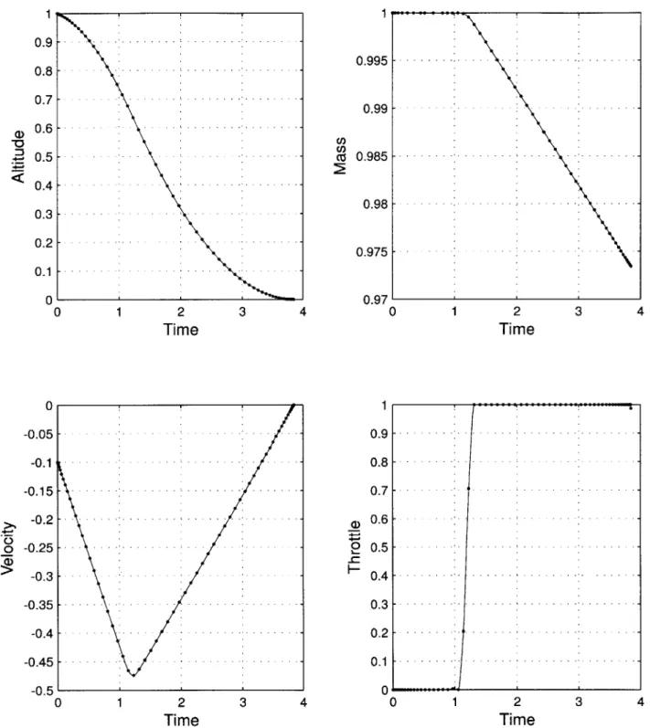
A total of 64 nodes was used for this simple case because a switch in the control is expected in the middle of the time span, where there are inherently fewer nodes. The number of nodes was increased (to 64) until this switch was adequately captured. The local minimum fuel solution is shown in Figure 2-4. It can be seen that the minimum fuel solution is a free fall trajectory until the point where a maximum commanded throttle, during the remaining portion of the descent, is sufficient to stop the vehicle the instant it reaches the surface. This is the intuitive solution since tf is also minimized in this fashion. By indirectly minimizing the time, less thrust is expended to counteract gravity.
In Figure 2-4, the discretized DIDO solution is plotted as points. As a feasibility check, the initial conditions are propagated forward using MATLAB's Runge-Kutta integrator (ode45), with the discretized control determined by DIDO. In this plot, the solid line represents either the interpolated control or the propagated state. The alignment of the propagated state (solid line) with the DIDO predicted state at the nodes verifies the
feasibility of the solution.
The Hamiltonian, as defined in Equation (2.20), is found to be:
'H = Ay(v) + Av max k g) + Am( max k (2.35)
( m Vex
Using Equation (2.24), the dynamics of the costate are determined to be:
A= 0 (2.36)
= -Ay (2.37)
= Av Tmaxk (2.38)
The DIDO output includes estimates of both the Hamiltonian and the costate. These are plotted in Figure 2-5. A divergence is seen in the Hamiltonian and costate estimates at the boundaries of the time domain. This is an artifact of the current DIDO implemen-tation of the Legendre Pseudospectral Method.
Because the Hamiltonian is not a function of time, it should be constant over the entire time span. Looking at Figure 2-5, the estimate of the Hamiltonian is fairly small, but oscillations are present. A larger fluctuation is seen where the throttle switch occurs, because of the discontinuity in the control. An interior discontinuity in the state or control is not handled as well by a spectral method.
Looking at Equation (2.36), AY should also be constant with time. An oscillation is also seen, but a flat trend is apparent. A, on the other hand, should have a constant slope equal to -AY, which is reflected in the plot. These simple tests show that the estimates of the Hamiltonian and costate are reasonable.
Since the Hamiltonian is a linear function of the throttle, Pontryagin's Minimum Principle must be used to determine the control. To find the control which minimizes the Hamiltonian at each node, each term in the Hamiltonian that is a function of the throttle is extracted and k is factored out. This is known as the switching function, which
1 msses1 0.9 -- - - -0.995 - . 0.8 - --0.7 - . - - -- - ... .. .. ... .. .. .. 0.99 0.6 . .. .. S 0 .5 - . . . . . -.. . . -.. . .. . c 0 .9 8 5 -- -- -- - - --- --- -0 .4 - .. . . . . -.. . .. . . 0.98 - . . . . --0 .3 - .. . . .. . . . -- --0.2 - - -0.975 - -0.1 - -0 0.97 0 1 2 3 4 0 1 2 3 4 Time Time 0 1 -0.05 - 0.9 - --0.1 - - 0.8 - ----0.15 0.7 -0.2 - 0.6 -o-0.25 - 0.5 - -... -0.3 - 0.4 -0.35 ... ... 0.3 ... ... -0.4 - - - 0.2 - --... -0.45 - - - 0.1 --- --0.5' 0 0 1 2 3 4 0 1 2 3 4 Time Time
Figure 2-4: Vertical Descent Minimum Fuel Solution (Normalized Units)
x 10 12 10 8 6 4 -2 --2 -4--6 -0 1 2 3 4 Time E 1 2 3 4 Time -0.7 - -0.75--0.8 -0.85 -0.9- -0.95--1 . -1.05 -0 1 2 3 4 Time
Figure 2-5: DIDO Estimated Hamiltonian and Costate (Normalized Units) 0.02 0.018 0.016 0.014 0.012 0.01 0.008 0.006 E Iz
-
--- - - -- - -- -.- ---
-
-0 1 2 Time 3 4 0 -0.01 -0.02 -0.03 . -0.04- -0.05--0.06 -0
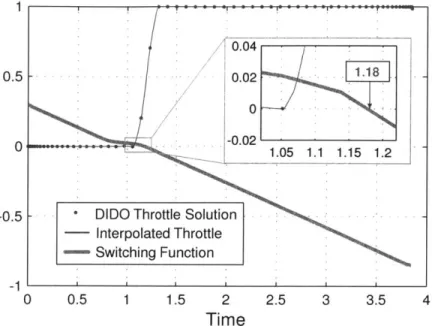
- DIDO Throttle Solution - Interpolated Throttle - Switching Function 0 0.5 1 1.5 2 Time 2.5 3 3.5 4
Figure 2-6: Estimated Switching Function
is written as in Equation 2.39 for this example.
(2.39)
By Pontryagin's Minimum Principle, the control is:
(2.40)
The DIDO estimates of the costate were used to calculate an approximate switching function. The result is plotted with the control in Figure 2-6. Using a cubic interpolation between the nodes, an estimate of the location where the switching function crosses zero is 1.18 in normalized time units. Thus, the obtained solution coincides with the estimated switch.
The next logical step is to split the problem into two distinct segments and allow for a discontinuity in the control. This is done in DIDO with the use of knots. Knots can also be used if there are discontinuities in the state (e.g., finite mass jumps in the ascent of a multi-stage rocket). For this problem, the state is equated at the knot, while the throttle
36 0.5 01 -0.5 1--1 S Av Tmax - AmTm"x m Vex ) k(t)
{
S> 1, S < 0 1F0
Knot Location 64 0 Knots 12 1 12 1 Knot to ti tf TimeFigure 2-7: Knot Inclusion
is allowed to be discontinuous. Fewer nodes are needed, as seen in Figure 2-7.
A guess of the knot time was provided to the optimizer as 1.18, but this time was
allowed to vary. The optimal solution found with one knot added is seen in Figure 2-8. The switch occurred at a normalized time value of 1.19. Therefore, the estimate of the switch location (calculated using an estimate of the costate and the derived switching function) is consistent with the knot location selected by DIDO.
To verify the result obtained from DIDO, an analytic solution is calculated from the method derived by Meditch [11]. He shows that there is no more than one switch in the throttle for the 1-dimensional vertical descent problem, and that the throttle changes from minimum to maximum at the switch. Using Pontryagin's minimum principle, Med-itch derived an analytic expression to calculate the time where the swMed-itch occurs. The expression is shown below in Equation (2.41). In deriving this equation, an assumption is made that no more than 25% of the initial mass is used as propellant during the descent. This assumption is valid for this example.
b y(t)
N(y,
v, t) = - y(t) + 2a + v(t) (2.41)1 ... 1 0.9 - -0.8 -.. 0.995 - -0 .7 - . . - . 0.6 . - 0.99 -- -. . Cl) 0.4 - 0.985 - ---0.3 .. . . 0.2 - -... .0.98 - -.-.-0.1 - -0 0.975 0 1 2 3 4 0 1 2 3 4 Time Time 0 1 -0.05 -0.9 - --0.2 - - - 0.8 - - --0.82 ... .. .. --- --- 0.5---0.15 - - 0.7 -0.2 . . 0.6 - -_ -0.25 ---- ----o-0.5.-.-... .o 0.5 . . --0 .3 -. . .. .-. -- -- .4. . .. .. . . . . -0 .3 5 - --- - -- -- .. .. . .. . 0 .3 - - -- -- --0 .4 - .. . . .-. .- ..- ..- 0 .2 - -.. .-. -0 .4 5 - - - - --- -- -. 1-- ---- ---0.5 0 0 1 2 3 4 0 1 2 3 4 Time Time
Figure 2-8: Vertical Descent Solution With One Knot (Normalized Units)
where a ( Tmax-mo (2.42) 2 mo T 2 b= 2 ax (2.43) 2Ve x mo2
The analytical solution placed the switch location at a normalized time of 1.21. The DIDO solution matches the analytical solution of the switching time, within a reasonable error of 1.6%. This simple vertical descent example has shown that solutions obtained by DIDO are good approximation of the optimal solution.
In the subsequent chapters, a soft-landing on the Moon from a parking orbit is ana-lyzed using the same DIDO optimization utility. An optimal solution is first obtain with minimum constraints and no interior knots in order to analyze the optimality of the re-sults and get an estimate of control discontinuity locations. The current implementation of DIDO does not provide estimates of the costate and Hamiltonian if interior knots are included, hence this analysis can only be performed with a solution that does not include knots. Knots are then added to the optimization framework in order to accurately capture control discontinuities, and to enforce desired characteristics of the trajectory based on operational considerations.
Chapter 3
Moon Landing Problem
This chapter presents details of the Moon landing scenario being investigated. Included within are assumptions made, coordinate frames used, definitions of terms, and an overview of the trajectory.
3.1
Assumptions
The rotational period of the Moon about its own axis is equal to the period of revolution around the Earth. The equatorial surface velocity is approximately 4.6 m/s. This rotation would be a factor if the goal was to target a specific landing site because the site would move relative to the inertial frame. However, a target is not specified in this analysis and it is reasonable to neglect the rotation of the Moon. The extra fuel expenditure required to null the velocity of the vehicle relative to the rotating surface would be no more than 0.3% of the total fuel usage. This is not a significant factor and would not noticeably alter the results or trends.
The Moon has no atmosphere and is assumed to be spherical. A purely Newtonian gravity model is used, therefore gravity perturbations due to the Earth and Sun are neglected, as well as perturbations due to the oblateness of the Moon. Values used for the lunar equatorial radius, Req, and the lunar gravitational parameter, y, are 1737.4 km and 4902.78 km 3/S2, respectively [26].
me-iz
bx bz
Figure 3-1: Three-Dimensional Inertial and Body Reference Frames
chanics problems because the properties of the engine do not change drastically in the operational range being used.
3.2
Reference Frames and Coordinate Systems
Three reference frames are used: the Inertial frame, the Vehicle Body frame, and a Ro-tating Polar frame. Where ambiguity is present, the frames are denoted with superscripts
(
)i(
)b and(
)",
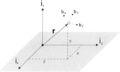
respectfully.The standard unit vectors, i, ily, and i, complete the inertial triad as seen in Figure 3-1. In this frame, the position vector, r, is expressed as:
r = xiz + Yiy + ziz (3.1)
The body frame is fixed to the vehicle and is given by the 3-dimensional unit vector triad
[br, by,
bz].
For a majority of the research done, the motion of the vehicle is restricted to a single plane of motion, namely the Moon's equatorial plane. If we define the x-y plane as the plane of motion, the inertial frame simplifies to the perpendicular unit vector set [i,
lU].
The body frame also reduces to the 2-dimensional perpendicular unit vectors[$X,
by]. An illustration of this is seen in Figure 3-2. The position vector reduces from Equation (3.1)yby
A
x
r
ix
Figure 3-2: Two-Dimensional Inertial and Body Reference Frames
yy
xI
Figure 3-3: Two-Dimensional Inertial and Rotating Polar Frames
to Equation (3.2).
r =
i
+ yiy (3.2)By defining unit vectors ir and io as in Equations (3.3) and (3.4) a rotating reference frame is created. This frame rotates at the same rate that the vehicle revolves around the Moon. It is referred to as the 'rotating polar frame' because of it is connection with the polar coordinates r and 6.
Ir= cos 6i + sin OiY (3.3)
io - sin Oiz + cos 6iY (3.4)
Figure 3-3 displays the relationship between the rotating polar frame and the inertial frame (for planar motion). The vector ir always points from the origin to the vehicle and
io remains perpendicular to the radius vector in the direction of motion of the vehicle. The position vector can be expressed rather simply in the rotating polar frame as:
iP
ha ra -hp Unoccupied Occupied Focus FocusFigure 3-4: Orbital Dynamics Definitions
3.3
Orbital Dynamics Definitions
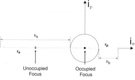
Standard orbital dynamics definitions [27] used in this document are displayed in Figure 3-4. The unit vectors
le
and i, lie in the vehicle's orbital plane withle
in the direction of the pericenter, which is the point of closest approach of the orbit to the occupied focus.i, is perpendicular to
le
in the plane of motion of the vehicle.In the case of a lunar orbit, the pericenter is referred to as the perilune. The vector from the occupied focus to the perilune is defined as the perilune radius vector, rp. The altitude at this point above the surface is referred to as the perilune altitude, hP. Conversely, the farthest point in the orbit is known as the apolune and the associated altitude is the apolune altitude, h,.
With the position and velocity of the vehicle are denoted by r and v, the perilune and apolune heights can be calculated using the following equations [27]:
h = r x v (3.6) e = (v x h - - r (3.7) y r h 2 P= - A- (3.8) p1 44
iy
V
/
\
,ix
Figure 3-5: Thrust Angle Definitions
Perilune Apolune
r -, r = (3.9)
1 +e 1-e
h= rp - Req ha = ra - Req (3.10)
where h and e are the massless angular momentum and eccentricity vectors, y and Req are the lunar gravitational parameter and equatorial radius, and p is the parameter of the orbit, which is defined by Equation (3.8). The variables r, h, and e denote the magnitudes of the corresponding vector. Note the distinction between hP and ha, which both represents
altitudes, and h, which is the magnitude of the massless angular momentum.
3.4
Angle Definitions
The planar equations of motion in both the cartesian and polar frames use a thrust direction angle, V), to represent the angular distance from a reference axis to the unit thrust vector. The cartesian equations of motion (EOM) uses i, which is defined from the fixed inertial x-axis. It is more convenient in the rotating polar frame to use V', which
is defined from the rotating radius vector. Figure 3-5 is included for clarity. Equation (3.11) relates the two angles. By taking the derivative of Equation (3.11) with respect to time, the relationship in Equation (3.12) is obtained.
iy
V IUT
4
L ix
F
Figure 3-6: Angle Definitions
+ (3.12)
For plotting purposes, the flight path angle, -y, and thrust direction angle, r, are defined. These angles are illustrated in Figure 3-6. The flight path angle, y, is the angle between the velocity vector and a line perpendicular to the radius vector in the direction of motion, which is referred to as the local horizontal. The unit thrust vector is defined with a yaw-pitch angle sequence, which is defined as a rotation about the radius vector by the angle r3
T and then a rotation about the z-axis (for the planar motion case) by the angle r/. The thrust yaw angle,
#T,
is defined from the direction of positive velocity. The thrust direction (pitch) angle, r, is the angle between the thrust vector and the local horizontal. The dotted vectors in Figure 3-6 show typical placements of the velocity and thrust vectors for the cases in this study.3.5
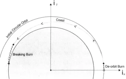
Trajectory Description
A vehicle that transfers from the Earth to the Moon arrives on a hyperbolic trajectory (when viewed from the vicinity of the Moon) by the laws of Keplerian motion. It is the