Coupling of a multizone airflow simulation program with computational fluid dynamics for indoor environmental analysis

Coupling of a Multizone Airflow Simulation Program with Computational Fluid Dynamics

for Indoor Environmental Analysis

by Yang Gao

M.S., Environmental Engineering University of Pittsburgh, 2000

Submitted to Department of Architecture in partial fulfillment of the requirements for the degree of

Master of Science in the field of Building Technology

at the

Massachusetts Institute of Technology June 2002

0 2002 Massachusetts Institute of Technology. All rights reserved.

Signature of Author cartment of Architecture " '~ 10, 2002 Certified by m 1 1aEyan Chen

Associate Professor of Building Technology Thesis supervisor

Accepted by

Stanford Anderson Head, Department of Architecture Chairman, Departmental Committee on Graduate Students

MASSACHUSETTS INSTITUTE

OF TECHNOLOGY

JUN 2 4 2002

LIBRARIES

Coupling of a Multizone Airflow Simulation Program with

Computational Fluid Dynamics for Indoor Environmental

Analysis

by Yang Gao

Submitted to the Department of Architecture on May 10, 2002 in partial fulfillment of the requirements

for the Degree of Master of Science in the field of Building Technology

ABSTRACT

Current design of building indoor environment comprises macroscopic approaches, such as CONTAM multizone airflow analysis tool, and microscopic approaches that apply Computational Fluid Dynamics (CFD). Each has certain advantages and shortfalls in terms of indoor airflow simulation. A coupling approach that combines multizone airflow analysis and detailed CFD airflow modeling would provide complementary information of a building and make results more accurate for practical design.

The present study attempted to integrate such building simulation tools in order to better represent the complexity of the real world. The overall objective of this study was to couple an in-house CFD program, MIT-CFD, with a multizone airflow analysis program, CONTAM.

Three coupling strategies were introduced. The virtual coupling makes use of the CFD simulation results in a large scale to provide boundary conditions for CONTAM. The quasi-dynamic strategy assumes that CFD can produce a "true" flow pattern and the CONTAM results should be changed accordingly. The dynamic coupling realizes an active two-way interaction between CFD and CONTAM through a bisection search procedure designed by the author that forces the airflow rates from the two models to converge.

Various case studies were conducted to validate the coupling strategies. Preliminary results show that all three coupling schemes can result in more reliable airflow patterns. Further investigations are needed to improve the coupling procedures and to apply to more generalized and complex real-world cases.

Thesis Supervisor: Qingyan (Yan) Chen

ACKNOWLEDGEMENTS

I would like to express my sincere thanks to my advisor, Prof. Qingyan (Yan) Chen for offering me the great opportunity to work on this project. My thanks are extended for his tireless support, great advice and consultation throughout the work. He has always given me valuable ideas and encouragement in completion of this thesis. His high standards and deep knowledge in research have provided me the most valuable help in the work.

I would also express my cordial gratitude to the other faculty members in Building Technology program, Professor Leon Glicksman, Professor Les Norford and Professor John Felnandez, for their kindness and support. My sincere thanks extend to Professor Glicksman for his advice and help while I was working as his teaching

assistant.

I thank Dr. Yi Jiang and Zhiqiang Zhai for their precious help and generous technical support throughout the research. My special thanks to Dorrit Schuchter and Kathleen Ross for their logistic support. I would also like to thank all my colleagues in the Building Technology Program for their collaboration and friendship.

My sincere love and thanks to my parents, Mei Chen and Zhongshun Gao, my parents-in-law, Aiqing Ye and Zhiming Hu, and my dear sister, Haiyan Gao for their loyal love and support. Finally, I would like to express my deepest love and gratitude to my husband, Dr. Yuanlong Hu, for his love and timeless support.

DEDICATION

Table of Contents

A b stract ... . . 3

A cknow ledgem ent ... 5

D edication ... _{. .. 6}

T able of C ontents ... 7

L ist of Figures ... 11

L ist of T ables ... 15

Chapter 1 Introduction

1.2 Current Design Tools and Problems...18

1.2.1 Multizone Airflow Analysis Tools ... 18

1.2.2 C FD M odels ... 19

1.2.3 Integration of Multizone Models and CFD Models ... 19

1.3 O bjective of the Present Study .... . ... 20

1.4 Thesis Outline ... 21

Chapter 2 Multizone Airflow Analysis Program-CONTAM

2.2...A Multizone Model-CONTAM ... 23

2.2.1 O verview ... 23

2.2.2 Building Representation in CONTAM... 24

2.2.3 Theoretical Background ... 24

2.2.4 Solution M ethods... 27

2.2.5 Boundary Conditions...30

2.3 ...Applications of CONTAM ... 31

2.3.1 AIVC Three-Story Building Case...32

2.3.2 French H ouse Case... 34

2.3.3 90-degree Planar Branch Case ... 48

Chapter 3 Description and Validation of a CFD Program

3.1 Introduction ... 51

3.2 Governing Flow Equations ... 52

3.3 M athem atical M odels... 55

3.3.1 Two-equation Turbulence M odeling ... 58

3.3.2 Zero-equation M odel... 62

3.4 N um erical M ethods... 64

3.4.1 Integration of the Governing Equations and Numerical Schemes... 65

3.4.2 Solution Procedure ... 68

3.5 Boundary Conditions ... 69

3.6 CFD V erification and V alidation... 70

3.6.1 N atural Convection Case... 71

3.6.2 Forced Convection Case... 71

3.6.3 M ixed Convection Case ... 76

3.6.4 Duct-in-series... 77

3.6.5 90-degree Planar Branch Case ... 79

3.7 Conclusion Rem arks ... 82

Chapter 4 Coupling of CFD and CONTAM

4.2 Virtual Coupling by Extracting CFD Information... 83

4.2.1 Coupling Strategy... 84

4.2.2 Problem Definition...84

4.2.3 Case Study-Natural Ventilation for a Shanghai Residential Com plex... 84

4.3 Quasi-dynamic Coupling of CFD into CONTAM...90

4.3.1 Coupling Strategy... 90

4.3.2 Solution M ethods... 93

4.3.3 Case Studies... 97

4.4 Dynam ic Coupling of CFD into CON TAM ... 109

4.4.1 Coupling Strategy...109

4.4.2 Solution M ethods...109

4.4.3 Num erical Stability...112

4.4.4 Case Studies...113

4.5 Conclusion Rem arks ... 122

Chapter

5

Conclusions and Future Work

5.1 Conclusions...124

5.2 Future W ork ... 126

List of Figures

Figure 2.1. Illustration of building idealization in CONTAM (NIST)...24

Figure 2.2. Cross-section of the AIVC three-story building...32

Figure 2.3. Plane view of each floor of the AIVC building and CONTAM simulation Results. Blue bars represent airflow rates, and red bars denote pressure ... 33

Figure 2.4. Simulation results-mass flow rates through the leakage paths ... 34

Figure 2.5. Mozart House floor plan from "Catalogue de Logements-Types" (de Montureux 1996) used in the case study ... 35

Figure 2.6. CFD model adaptation of the Mozart House including furniture types ... 36

Figure 2.7. CONTAM idealization of Mozart House based on adapted CFD model...36

Figure 2.8. Occupancy scenario for each person spent at home...37

Figure 2.9. Exhaust rates for the bimodal system showing an increase of the kitchen exhaust rate during cooking; and constant bathroom and WC exhaust in sum m er... . . 40

Figure 2.10.Exhaust rates for the RHC case in summer ... 41

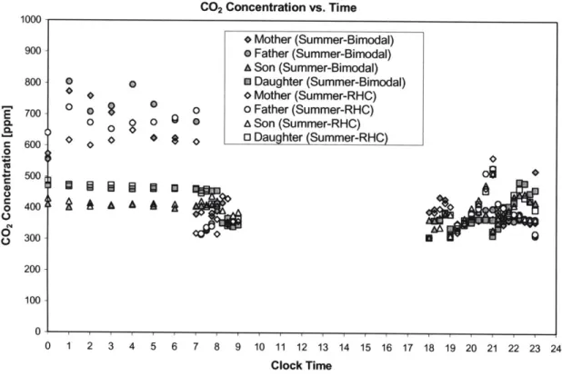
Figure 2.11 .C02 concentration history for bimodal ventilation in summer ... 44

Figure 2.12.CO₂ concentration history for RHC ventilation in summer ... 44

Figure 2.13.CO₂ concentration history of bimodal and RHC ventilation in summer obtained from CFD simulation (Huang 2001)...45

Figure 2.14.Water vapor concentration history for bimodal ventilation in summer ... 45

Figure 2.15.Water vapor concentration history for RHC ventilation in summer ... 46

Figure 2.16.Water vapor concentration history of bimodal and RHC ventilation in summer from CFD simulation (Huang 2001)...46

Figure 2.17.CONTAM representation of exhaust systems on the roof of French house...47

Figure 2.18.Results of general airflow pattern obtained from CONTAM simulation...47

Figure 2.19.Detail airflow pattern obtained from CFD by Huang (2001)...48

Figure 2.20.90-degree planar branch configuration...49

Figure 2.21.90-degree planar branch represented as airflow paths ... 49

Figure 2.22.90-degree planar branch represented as ducts...49

Figure 3.1. A typical control volume centered at node P...59

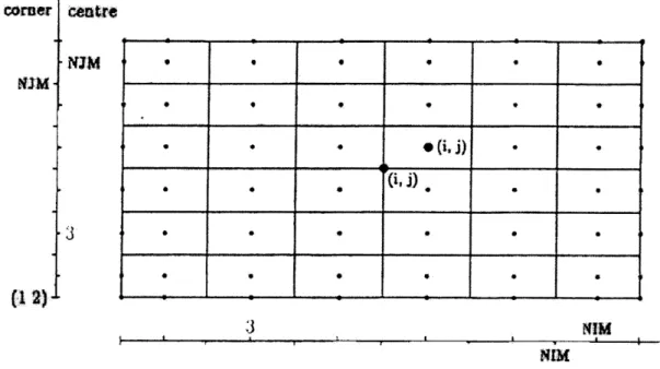
Figure 3.2. Layout and indexing of cell center and corner points ... 65

Figure 3.3. Nodes required by convection schemes in xr-direction ... 66

Figure 3.4. Sketch and boundary conditions of the natural convection case...72

Figure 3.5. Comparison of the airflow patterns for natural convection: (a) zero-equation model, (b) standard k-E model, (c) the Lam-Bremhorst low-Reynolds-number k-s model, (d) smoke visualization ... 73

Figure 3.6. The sketch of the forced convection case...74

Figure 3.7. Comparison of the airflow patterns for the forced convection: (a) zero-equation model, (b) the standard k-& model ... 74

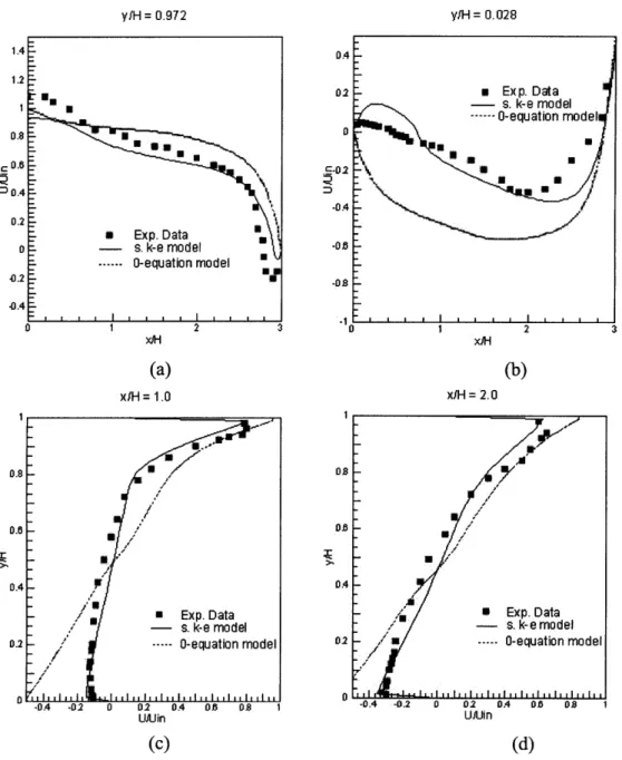
Figure 3.8. Comparison of velocity profiles in different sections of the room with forced convection ... 75 Figure 3.9. Comparison of the airflow patterns for the mixed convection: (a) the

(b) the zero-equation model in MIT-CFD ... 76

Figure 3.1O.Comparison of the penetration length vs. Archimedes number for the room with m ixed convection ... 77

Figure 3.11 .Schematics of the three horizontal parallel-plate ducts in series...78

Figure 3.12.Airflow along the 5m -duct ... 78

Figure 3.13.Comparison of computational results and analytical results of the duct...79

Figure 3.14.Contours of streamline velocity pattern: (a) Re=10, (b) Re=300...80

Figure 3.15.Fractional flow rate in main branch as a function of Reynolds number ... 82

Figure 4.1. Site plan in Shanghai, China ... 85

Figure 4.2. Location of single-level apartment and duplex apartment in the study...86

Figure 4.3. Single-level apartm ent... 87

Figure 4.4. Airflow pattern simulated by CONTAM and CFD...87

Figure 4.5. The layout of the duplex apartment in Shanghai building complex...89

Figure 4.6. The general airflow pattern predicted by CONTAM and CFD...89

Figure 4.7. Decouple a mass flow network from a CFD domain as presented in N egrao (1995)... . 91

Figure 4.8. Illustration of the coupling between CFD and CONTAM ... 93

Figure 4.9. Quasi-dynamic coupling flow chart ... 96

Figure 4.1 O.Illustration of discretized combined computational domain for 3-duct-in-series ... 97

Figure 4.11 .CONTAM presentation as airflow paths...98

Figure 4.12.CONTAM presentation as ducts ... 98

Figure 4.13.Illustration of a 90-degree branch using coupled method ... 100

Figure 4.14.90-degree planar branch case: (a) airflow pattern before coupling, (b) airflow pattern after coupling...100

Figure 4.15.Airflow rate through each opening in 90-degree planar branch before and after quasi-dynam ic coupling...102

Figure 4.16.4-zone configuration modified from 90-degree planar branch case...103

Figure 4.17.Modified 90-degree planar branch case 1(4 zones)...103

Figure 4.18.Airflow rate through each opening in modified 90-degree planar branch case 1 (4 zones) before and after quasi-dynamic coupling ... 105

Figure 4.19.6-zone configuration modified from 90-degree planar branch case...106

Figure 4.20.Modified 90-degree planar branch case 2 (6 zones): (a) airflow pattern before coupling (numbers in the figure indicate the path identification); (b) airflow pattern after coupling ... 107

Figure 4.21 .Airflow rate through each opening in modified 90-degree planar branch case 2 (6 zones) before and after quasi-dynamic coupling ... 108

Figure 4.22.Dynam ic coupling flow chart ... 110

Figure 4.23.Special procedure in dynamic coupling seeking new coefficients of powerlaw relation that will minimize the airflow rate difference of CONTAM and CFD simulation...111

Figure 4.24.Dynamic coupling-modified 90-degree planar branch case 1 (4 zones) (a) airflow pattern before coupling. Air path identification numbers are also indicated; (b) airflow pattern after coupling...113 Figure 4.25.Airflow rate through each opening in modified 90-degree planar branch

Case 1 (4 zones) before and after quasi-dynamic and dynamic coupling...114 Figure 4.26.Dynamic coupling-modified 90-degree planar branch case 2 (6 zones):

(a) airflow pattern before coupling. Air path identification numbers are also indicated; (b) airflow pattern after coupling...115 Figure 4.27.Airflow rate through each opening in modified 90-degree planar branch

Case 2 (6 zones) before and after quasi-dynamic and dynamic coupling.... 116

Figure 4.28.Three-dimensional presentation of the modified forced convection case .... 118

Figure 4.29.Modified forced convection case-room geometry (Musser 2001)...118 Figure 4.30.Non-dimensional velocity profile for room 1 and 2 by using CFD

simulation only and by using the coupled program (CFD+CONTAM) opening height = 0.09m. The upper three panels show the results where room 2 is being coupled; the lower three panels are the results when

room 1 is being coupled ... 119 Figure 4.31 .Non-dimensional velocity profile for room 1 and 2 by using CFD

simulation only and by using the coupled program (CFD+CONTAM) opening height = 0.59m. The upper three panels show the results where room 2 is being coupled; the lower three panels are the results when room 1 is being coupled...120 Figure 4.32.Non-dimensional velocity profile for room 1 and 2 by using CFD

simulation only and by using the coupled program (CFD+CONTAM) Opening height = 2.24m. The upper three panels show the results where room 2 is being coupled; the lower three panels are the results when

List of Tables

Table 2.1. D aily activity of occupancy ... 37

Table 2.2. Description of indoor contaminants used ... 38

Table 2.3. Strengths of pollutant sources used in the simulations ... 38

Table 2.4. Strength of vapor source used in the simulation...38

Table 2.5. Exhaust flow rate for bimodal ventilation ... 39

Table 2.6. Minimum and maximum flow rates of the humidity controlled ventilation system (RH C) ... 39

Table 2.7. Ventilation rate changes by controlled humidity...39

Table 2.8. Window leakage area in each room obtained from CFD simulation...42

Table 2.9. Comparison of individual room air change rate (ACH) computed by CFD and CONTAM from 18:00 - 19:00...42

Table 2.10.Comparison of individual room ACH computed by CFD and CONTAM from 19:00 - 21:00 ... 43

Table 3.1. The standard k-s turbulent model parameters in the individual equations ... 61

Table 3.2. Numerical schemes implemented in MIT-CFD program...67

Table 3.3. Mass flow rate at the opening under different Reynolds numbers ... 81

Table 4.1. Pressure distribution at each window opening ... 87

Table 4.2. Comparison of the air change rates computed from CONTAM and CFD for single-level apartm ent ... 88

Table 4.3. Comparison of the air change rates computed from CONTAM and CFD for duplex apartm ent ... 90

Table 4.4. CONTAM mass flow network results compared to ESP-r dps results...99

Table 4.5. Results from the combined approach using different models in CFD-side...99

Table 4.6. Results of a 90-degree planar branch by quasi-dynamic coupling ... 101

Table 4.7. Results of the modified 90-degree planar branch case 1 (4 zones) by quasi-dynam ic coupling ... 104

Table 4.8. Results of the modified 90-degree planar branch case 2 (6 zones) by quasi-dynam ic coupling ... 108

Table 4.9. Results of the modified 90-degree planar branch case 1 (4 zones) by dynam ic coupling...114

Table 4.1 0.Results of the modified 90-degree planar branch case 2 (6 zones) by dynam ic coupling...116

CHAPTER 1 INTRODUCTION

1.1 General Statement of Problem

Since the emergence of the first air-conditioning system designed by W.H. Carrier (1902), people are more and more dependent on indoor climate. At present, people in developed country spend about 90% of their time indoors. Building environmental issues has therefore received more public attentions than ever. "Healthy building" design now becomes the main stream on the verge of a paradigm shift in building ventilation design thinking (Spengler and Chen, 2000).

In the past three decades, the design of indoor environment has undergone several major shifts. In respond to the energy crisis in the 1970s, energy-efficient building concept drove engineers to design more insulated, airtight and less ventilated buildings since building consumed one third of total energy in developed country. Although those energy-efficient measures saved huge amount of energy, the heavy trade-off was insufficient ventilation maintaining a benign indoor environment. Therefore, as a relatively independent ecosystem, indoor environment could not provide well-diluted

clean air and desirable thermal comfort level in certain spaces.

On the other hand, many sources of contaminants, such as volatile organic compounds (VOCs) and radon, are introduced to working and living indoor environment. As consequences, indoor air quality (IAQ) becomes impoverished due to inadequate air infiltration or insufficient fresh air supply. Poor IAQ may lead to "Building-Related Illness" and "Sick Building Syndrome", which may have acute or chronic effects on human health. People have growing awareness of health risks from poor IAQ (Molhave 1982, Esmen 1985, Nero 1988). For example, increased cancer risk has been linked to poor IAQ (Spengler and Chen 2000). This leads to an increased minimum fresh air rate for each occupant defined in ASHRAE (American Society of Heating, Refrigerating and Air-Conditioning Engineers, Inc.) Standard 62 (1999) for acceptable indoor air quality.

Moreover, poor IAQ is being blamed for problems of low worker productivity and therefore associated with significant economic loss. According to several studies, impoverished IAQ causes an average 10% loss of productivity, and a widely accepted, conservative value of 6% (Dorgan et al. 1998). The overall economic losses due to poor IAQ in US commercial buildings are estimated to be about $20 to $160 billion per year (Fisk 2000). Although poor IAQ is not a sole contributor to health problems, productivity and economic loss, it declares the fact that "safe" and "benign" interior environment is no longer existing in current modem society. Buildings are now a source of contamination due to the fact that it may actually be more polluted than the surroundings (Spengler and Chen 2000).

Changes in construction, materials, energy cost, and health concerns are shifting ventilation philosophy once again. Health, economics, and aesthetics are becoming more important than comfort in determining the specification for ventilation (Spengler and Chen, 2000). "Healthy" building design requires the consideration of good IAQ and thermal comfort as well as energy-efficiency. This has stimulated the development of new technologies, such as natural ventilation and low energy cooling. The analysis of those new technologies requires tools that can be both sophisticated and simplified as need.

1.2 Current Design Tools and Problems

Modern buildings and their heating, ventilation and air-conditioning (HVAC) systems are required to be both energy- and environmental-conscious. In the last decade, computer design tools have been promoted due to the pressure on designers to perform quick design. Most of computer applications focus only on one or two design aspects, such as load calculations, energy consumption estimation, duct design, pipe design, etc. (Lebrun 1994). However, building indoor air quality and HVAC design is a complex task consisting of various interactive factors that requires experts from different disciplines

(Ellis and Mathews, 2002).

The design of acceptable indoor air quality should meet ASHRAE standards 62-1999. Current design simply uses a single value for indoor air parameters, which is a representation often used by multizone or zonal models. In most cases, however, the air within a single room is not well mixed and may have gradient within. Thus, a single value cannot well represent local thermal comfort and air quality. On the other hand, there have been extensive efforts in applying Computational Fluid Dynamics (CFD) to indoor environmental study that may offer detailed IAQ information within a room. This leads to the possibility of integrating these two types of computational tools, i.e., multizone and CFD models, for indoor airflow analysis. In which follows, a brief introduction on each tool categories is given.

1.2.1 Multizone Airflow Analysis Tools

Some indoor air quality problems require the airflow analysis of a whole building driven by pressure difference or temperature difference. Currently, the design of acceptable indoor air quality is according to ASHRAE standard 62-1999 that uses a single value for indoor air quality parameters. Multizone airflow network models become a common tool to provide such indoor air quality information.

Multizone airflow network model calculates air exchange and contaminant migration within the rooms of a building and between a building and outdoors (Schaelin 1993). These models typically represent the rooms of a building as zones with homogeneous air properties and contaminant concentrations. Airflows are described as airflow paths that interconnecting with each other and have user-defined leakage

characteristics (Musser, 2001). By mass balance, the airflow rates through paths and the averaged contaminant concentrations are evaluated. Although a number of assumptions must be made regarding envelope leakage characteristics and weather conditions, multizone models have been used to represent many types of buildings with acceptable

accuracy (Furbringer et al. 1996)

1.2.2 CFD Models

In real world, however, the air within a single room is not well mixed but varies spatially. Air temperature and contaminant concentration therefore are distributed with gradient. This is especially true for large spaces, such as atria and lobbies; and for buildings with non-mixing ventilation systems, such as displacement ventilation and natural ventilation. A single value cannot well represent local thermal comfort and air quality. Therefore, multiple values that can reflect non-homogeneous condition in a room is necessary for proper indoor air quality and HVAC design.

Such characteristics can be captured by CFD techniques. In CFD analysis, room is divided into numerous grids, and the nonlinear partial differential equations that govern the airflow, heat and mass transfer in a space are discretized and solved numerically. A detailed description of air velocities, air temperature, and contaminant concentrations is therefore obtained. Theoretically, CFD can be applied to whole building airflow analysis. However, such endeavor is not attempted to achieve due to huge computer resources involved even for a simplified building geometry. Therefore, CFD analysis has historically been limited to flows in single spaces or small sets of rooms where detail information is needed rather than entire buildings (Musser 2001).

1.2.3 Integration of Multizone Model and CFD Models

A modeling approach that combines multizone airflow analysis and detailed CFD airflow modeling would provide complementary information of a building and make results more accurate for practical design. The integration of multizone and CFD models has therefore been investigated in several studies.

A link between multizone models and CFD can be in a two-way sense. One is to supply the calculated airflow information from a CFD model into multizone models. The other is to perform CFD calculation using boundary conditions obtained from a multizone model simulation. Schaelin et al. (1993) demonstrated a method to include the CFD results from detailed single-room calculation into multizone models for a more adequate description of real cases. The method worked for a whole building with one room for CFD calculation. And the interface parameters of this room were transferred between the CFD program and the multizone program with manual iteration. The whole procedure was called a "ping-pong" technique.

More recently, Musser (2001) investigated the impact of room representation and boundary conditions on predicted contaminant concentrations and airflow profiles in a set of two isothermal rooms connected by an opening with varying sizes. The study compared four possible combinations of the multizone and CFD model assembly: multizone only, CFD only, CFD for the first room and multizone for the second room, and multizone for the first room and CFD for the second room. Although this investigation confirmed that the multizone models could not accurately predict the airflow and contaminant level in a poorly mixed room, the two programs were just manually combined. Nevertheless, this study suggests the combination of CFD and multizone models is desirable when a critical room is poorly mixed.

One attempt in dynamically coupling CFD with multizone network model was conducted by Negrao (1995). He implemented a CFD algorithm within the ESP-r module that is a building energy modeling system. Both ESP-r system and the CFD program that he used employed finite volume method. The conflation technique essentially treated the airflows across the openings as sources. The information exchange of such sources was conducted at every sweep of CFD solver iteration until the CFD convergence criterion was met. However, other multizone airflow network programs, such as COMIS and CONTAM, do not consider the source term in mass balance equation. Therefore, the coupling method developed in ESP-r may not applicable to other multizone programs if their original algorithm and data structure are to be maintained.

1.3 Objective of the Present Study

The discussion in the previous sections indicates the importance of integrating multizone airflow models and CFD models. Preliminary studies conducted by other researchers have also been briefly discussed. However, it suggests that different approach should be investigated in order to fully couple a CFD program with the most common multizone airflow analysis programs, such as CONTAM and COMIS. The present work will focus on the coupling of CFD with one of such multizone programs, in this case, CONTAM, because it has received more attention for its validity and application.

CONTAM is a multizone airflow analysis program developed by National Institute of Standard and Testing (NIST) (Stuart Dols 2000). It is an object-oriented program written in C language with user-friendly interface, which becomes increasingly popular recently. Although the impact of combining CONTAM andCFD program was mentioned by Musser (2001), the real implementation of coupling a CFD program and CONTAM has never been realized.

Building Technology Program at the Massachusetts Institute of Technology has developed an in-house CFD program, called MIT-CFD. This program can solve a variety of three-dimensional airflow problems within a specific space, whether turbulent or laminar. The program has been developed to be user-friendly and it allows user to make changes for specific purpose. MIT-CFD is therefore chosen for the present study.

The overall objective of this investigation is to couple MIT-CFD with CONTAM and study the impact of the coupled program on airflow analysis. More specifically, the present study aims to:

e Validate MIT-CFD program for coupling needs.

* Apply CONTAM into indoor airflow and IAQ analysis.

* Develop a coupling procedure by MIT-CFD and CONTAM, and verify the techniques employed.

* Apply the coupled program for indoor airflow and IAQ studies.

1.4 Thesis Outline

The thesis can be outlined into the following chapters:

Chapter 2 introduces a multizone airflow analysis program-CONTAM and its theoretical background. The application of CONTAM is then discussed using case study approach. The limitation of CONTAM is therefore identified.

Chapter 3 reviews the fundamentals of MIT-CFD program followed by validating this program with experimental data.

Chapter 4 introduces three coupling strategies conforming to different research objectives and details; these include virtual coupling, quasi-dynamic coupling, and dynamic coupling. In virtual coupling, CFD simulation provides CONTAM pressure boundary information for the whole building simulation. Quasi-dynamic coupling focuses on the cases in which CFD simulation results is presumably correct and can fully impact the CONTAM simulation results. Dynamic coupling deals with the cases when CFD and CONTAM can communicate with each other during the simulation. After discussions on each coupling strategies, verifications are conducted to examine the coupling strategies. The applications of the coupled program for building airflow simulation are discussed and the engineering significance of the coupling between CFD and CONTAM is highlighted.

Chapter 5 summarizes the work presented in this thesis, and provides recommendations for future research.

CHAPTER 2

MULTIZONE AIRFLOW ANALYSIS PROGRAM-CONTAM

2.1 Introduction

The design to prevent indoor air quality problem and to meet space-conditioning loads for energy consumption requires the understandings of airflow pattern and the mechanisms of contaminant migration in an entire building. Traditionally, three hierarchical types of simulation tools are available for research purposes and engineering

applications: multizone models, zonal models, and CFD models.

Multizone IAQ modeling has been available as a research and analysis tool for over 20 years (Emmerich, 2001). The multizone models simulate airflow pattern from one zone to another in an entire building with only coarse structure information and assume uniform air parameters in a zone. The multizone models can provide designers gross information regarding indoor air quality in a building. Typical multizone models include CONTAM (Stuart Dols, et al. 2000) and COMIS (Pelletret and Keilholz 1997). Such models take a macroscopic view of air motion and contaminant dispersion, which enable the analysis of whole building airflow pattern and airborne contamination levels. Unfortunately, these models have great uncertainties when they are used to simulate large spaces, such as atria. This is because the air distribution in large spaces is not uniform.

CFD simulation divides a single zone into numerous small cells. By solving discretized mass, momentum, energy and species conservation equations, CFD generates detailed temperature, concentration and airflow field in a zone. The CFD approach is very powerful, but it would cost too much computing time if it were used to simulate indoor air quality problem within an entire building.

The zonal modeling acts as a bridge between the multizone macroscopic modeling and CFD microscopic modeling. The zonal model calculates the airflow pattern in a zone with limited subzones/nodes over which mass and energy conservation based on a number of approximations must be satisfied. Some of typical models are from Lebrun (1970), Inard et al. (1996), Howarth (1985), Togari et al. (1993), Rodriguez et al. (1994), Inard and Buty (1991), Wurtz et al. (1999), Haghighat et al. (2001), and Musy et al. (2001). For all the zonal models at present, assumptions must be made on inter-zonal airflow patterns. The use of zonal models thus requires a large competence in modeling and experimenting in buildings. Morover, for each different problem, a particular analysis is necessary to build a new cell arrangement and the whole set of equations have to been solved repeatedly. A recent review by Griffith (2002) found that most of the zonal models are unstable and need extensive prior knowledge of airflow pattern. It is very difficult to use zonal models for studying indoor air quality problem in an entire building.

Therefore, the integration of CFD into a multizone model would be ideal, since the CFD can provide accurate and detailed information for large spaces and the multizone model can simulate quickly on indoor air quality problem for an entire building. The following section will give an introduction and description of a specific multizone model program - CONTAM. Several applications of CONTAM will be discussed in section 2.3.

2.2 A Multizone Model - CONTAM

2.2.1 Overview

A 1992 survey reported that nearly fifty multizone network airflow models are used in industry and academic communities (Feustel and Dieris 1992). However, many of these were developed as in-house research tools, and only a few have been made available to the public. CONTAM is among these that are available to for public access and becomes increasingly popular recently. CONTAM includes graphical input and output interfaces, which is user-friendly. It also has the capacity to allow the user to specify schedules for occupants, contaminants, weather conditions, and HVAC system operation (Musser 2001). Therefore, it has been received more public attentions and is chosen for this study.

CONTAM is a multizone indoor air quality and ventilation analysis computer program designed to determine general airflow pattern, contaminant concentrations and personal exposure if needed. The model can be applied to a variety of applications, such as assessing the adequacy of ventilation rates in a building and obtaining the distribution of ventilated air throughout a building. It can also be used to predict contaminant concentrations so as to determine the indoor air quality performance for a building in its design stage or for an existing building, and to evaluate the impacts of various design decisions related to the ventilation system construction. Predicted contaminant concentration can also be used to estimate personal exposure based on occupancy patterns within the building.

The multizone network airflow model approach has been extensively evaluated using both analytical solutions and experimental data (Furbringer et al. 1996). Upham (1997) also reviewed past validation work and compared model predictions with tracer gas measurements taken in a five-story building. In her study, the predicted tracer gas concentrations by CONTAM were shown to within approximately 20% of true values. Deviations of this order of magnitude are commonplace in infiltration and contaminant prediction and have been deemed acceptable for many types of analysis (Persily and Linteris 1983).

2.2.2 Building Representation in CONTAM

To represent a building using the CONTAM model, the building must be simplified into a set of zones that represent individual rooms and spaces. CONTAM provides a macroscopic model for a building, that is, zones are treated as perfectly mixed volumes in the simulation. Figure 2.1 illustrates the process of building idealization that is presented by NIST in its CONTAM website in the division of building technology (http://www.bfrl.nist.gov/IAQanalysis/default.htm). In many applications, each room of a building can be represented as a single zone. These zones are connected to one another or

to ambient by airflow paths that represent the cracks, openings, fans, etc. The temperature of each zone and weather condition need to be specified in order to perform simulation. Optional inputs include contaminant sources and sinks, occupant schedules, and HVAC systems with ducts, filters, and recirculation.

Figure 2.1. Illustration of building idealization in CONTAM (NIST).

2.2.3 Theoretical Background

CONTAM requires the use of various assumptions in order to implement mathematical relationships to model airflow and contaminant dispersion. Firstly, each zone representing certain building space is treated as a single node, where the assumption of uniform (well-mixed) condition is employed. The uniform assumption treats zone temperature, pressure and contaminant concentrations as single values whereas the localized effects within a given zone are overlooked. Secondly, CONTAM does not treat heat transfer automatically. Users are responsible to manually set the temperatures in all zones. The model can only determine airflows induced by temperature differences between zones including ambient caused by stack effect. Moreover, empirical nonlinear mathematical models are utilized to represent the airflow paths to which the pressure drop relates. Other major assumptions include quasi-steady airflows, trace contaminants and source/sink models, etc.

A variety of air movement models have been developed for estimating airflows in buildings. These flows include infiltration, natural ventilation, inter-room airflows

through various openings including doorways and flows through the HVAC system (Walton, 1989). Infiltration is the result of air flowing through openings. These opening could be large or small, intentional or accidental in the building envelope. Infiltration is driven by pressure difference, Ap, across the opening. The relationship between the airflow through an opening in the building envelope and the pressure difference across it can be modeled in several ways in CONTAM.

It is assumed that Bernoulli's equation governs the flow within each airflow element.

AP = P + - P2 + P2 + pg(zi - z2

)

where,

AP = total pressure drop between points 1 and 2

P1, P2 = entry and exit static pressures VI, V2 = entry and exit velocities

p = air density

g = acceleration of gravity (9.81 m/s2)

Z1, Z2 = entry and exit elevations

In CONTAM, the pressure terms are rearranged and a possible wind pressure term for a building envelope opening is added:

AP = P - P + P, + P. (2.2)

where,

Pi, P; = total pressure at zones i andj

P, = pressure difference due to density and elevation differences, and P, = pressure difference due to wind.

P, is defined as Equation 2.3:

P. = P C, (2.3)

2

where

p =ambient air density

VH = approach wind speed at the upwind wall height

Ps is defined as Equation 2.4:

P = "Pn '" gAh (2.4)

2

where

P., Pm air density in zone n and m

g gravitational acceleration, 9.80 m2/s

Ah = elevation difference

Most infiltration models are based on the powerlaw relationship between the flow and the pressure difference across a crack or an opening in the building envelope. In CONTAM, three basic variations of power law relationship for turbulent flow are included: Q = C(AP)" (2.5) F = C(AP)" (2.6) Q = CdA (2.7) P Where,

Q

F= Mass flow rate [kg/s]

AP = the pressure drop

Cd = discharge coefficient, and

A = orifice opening area n = exponent constant

Theoretically, the value of the flow exponent constant should lie between 0.5 and 1.0. A variety of research indicates that n=0.5 characterizes large openings well, while n=0.65 can be used to describe crack-like openings.

Besides the powerlaw flow elements, CONTAM also enables calculation based

on quadratic relationship( AP=A Q+ BQ2, forQ, AP >0 AP = AQ - BQ2_{, for Q, AP < 0).} Baker et al. (1987) indicated that infiltration openings could be more accurately modeled by a quadratic relationship. Duct flow is treated based on 1997 ASHRAE Handbook of Fundamentals (1997), and CONTAM also includes special treatment of large openings

for possible two-way flow. In the present study, we only consider one-way flow through the openings, most of which can be represented by powerlaw relationship. Therefore, for the current stage of the coupling, only powerlaw airflow paths are considered.

To account temperature dependence in CONTAM, a correction factor to the base condition is used, according to the following formulae for computing air density, p, and dynamic viscosity, v:

p = P / (287.005) (2.8)

p = 3.7143x10-6 + 4.9286x10-'T (2.9)

v=p /P p(2.10)

The base conditions refers to standard atmospheric pressure and 20'C, where po= 1.2041 kg/m3 _{and vo = 1.5083x10-' m}2_/s.

2.2.4 Solution Methods

CONTAM calculates the infiltration and ventilation rates in a building by solving a non-linear system of equations (2.14) for all zones. An iterative method can be used in which a linear system of equation is solved in each step of the process. The Newton-Raphson method is often used for this kind of problem, which will be detailed later.

An airflow network consists basically of a set of pressure nodes (zones) connected by links, which are called airflow elements in CONTAM. The zones may represent rooms, connection points in ductwork, or the ambient environment. The airflow elements correspond to discrete airflow passages such as doorways, construction cracks, ducts, fans, and other openings. The airflow rate from zone

j

Fj =f(P - PI) (2.11)

The mass of air, mi [kg], in zone i is given by the ideal gas law:

mi = piV = PiV/ RT (2.12)

where

pi = air density in zone i [kg/m3_],

Vi= zone volume [m3

],

Pi = zone pressure [Pa],

T= zone temperature [K], and

R = 287.055 [J/kg-K] (gas constant of air).

dm. _Y

d = F + F (2.13)

dt

where

mi= mass of air in zone i,

Fj= airflow rate [kg/s] between zonesj and zone i: positive values indicate flows fromj to i and negative values indicate flows from i toj, and

Fi = non-flow processes (sources or sinks) that could add or remove significant quantities of air from the zone.

Sources and sinks are not considered in CONTAM and flows are evaluated by assuming quasi-steady conditions, dmi/dt = 0, which leads to:

F = 0 (2.14)

The steady-state airflow analysis of multiple zones requires simultaneous solution of equation (2.12) for all zones. Since the function in equation (2.9) is usually nonlinear, a method is needed to obtain the solution of simultaneous nonlinear algebraic equations. The Newton-Raphson (N-R) method (Conte, and de Boor 1972) is chosen in CONTAM to solve the nonlinear problem by iteration. In the N-R method a new estimation of the vector for all zone pressures, {P} *, is computed from the current estimate of pressures,

{P}, by

{C} (2.15)

where the correction vector, {C}, is computed by the matrix relationship

[J] {C} = {B} (2.16)

where {B} is a column vector with each element given by

B = EF (2.17)

And [J] is the square Jacobian matrix whose elements are given by

(2.18)

In equations (2.15) and (2.16), F,; and DFji/ Pj are evaluated using the current estimate of

which returns the mass flow rates and the partial derivative values for a given pressure difference input.

Equation (2.16) represents a set of linear equations, which must be set up and solved for each iteration until a convergent solution of the set of zone pressures is achieved. In its full form [J] requires computer memory for N2 values, and a standard Gauss elimination solution has execution time proportional to N3_{. Sparse matrix methods can be} used to reduce both the storage and execution time requirements. A skyline solution process following the method presented by Dhatt (1984) was utilized. This method can be applied to solve equations with symmetric or nonsymmetrical matrices. In this case, the Jacobian matrix is symmetric.

Analysis of the element model will show that

|Jul = E|Jijl (2.19)

j+i

This condition allows a solution without pivoting, although scaling may be useful. Note that the degree of sparsity of the Jacobian matrix after factoring is dependent on the arrangement of the zones. The CONTAM user interface ensures the correct interconnection the airflow elements in the network.

CONTAM allows zones with either known or unknown pressures. The constant pressure zones are included in the system of equation (2.14), which is processed so as not to change the pressure of the chosen zone. This gives flexibility in defining the airflow network while maintaining the symmetric set of equations. A sufficient condition for the Jacobian to be nonsingular is that the entire unknown pressure zones being linked, either directly or indirectly, by pressure dependent flow paths to a constant pressure zone. In CONTAM, the ambient (or outdoor) air is treated as a constant pressure zone (Axley, 1987). The pressure difference due to wind effect is considered in Equation 2.2 separately. The ambient zone pressure is assumed to be zero for the flow calculation causing the computed zone pressures to be values relative to the true ambient pressure and helping to maintain numerical significance in calculating AP.

Conservation of mass at each zone provides convergence criterion for the N-R iterations. That is, when equation (2.12) is satisfied for all zones for the current system pressure estimate, the solution has converged. Testing for relative convergence at each zone attains sufficient accuracy:

<8 (2.20)

with a test of }jFjlj < c to prevent division by zero. The magnitude of e can be established by considering the use of the calculated airflows, such as in the situation of an energy balance. In any case, round-off errors may prevent perfect convergence (e = 0).

To achieve faster and reliable convergence, a simple constant under-relaxation coefficient suggested by Walton (2000) and Wray (1993) is used. Equation (2.13) for the iteration becomes

{P}* = {P} - cO{C} (2.21)

where co is the relaxation coefficient. A relaxation coefficient of 0.75 has been found to be usable for a broad range of airflow networks. This value is not a true optimum but appears to work quite well without the computational cost of finding the theoretically optimum value.

When Convergence is progressing rapidly, under-relaxation (cO < 1) slows convergence compared to no relaxation. To prevent this, a global convergence value is computed:

y = (2.22)

EEj I Fj'j

when y* < ay, co is set to 1. Currently, CONTAM uses a = 30%. This often reduces the number of iterations.

Newton-Raphson's method requires an initial set of values for the zone pressures. These may be obtained by including in each airflow element model a linear approximation relating the flow to the pressure drop:

F,i = cjj + b,i(P - P) (2.23)

Conservation of mass at each zone leads to a set of linear equations of the form

[A] {P} = {B} (2.24)

Matrix [A] in equation (2.22) has the same sparsity pattern as [J] in equation (2.14) allowing use of the same sparse matrix solution process for both equations. This initialization handles stack effects very well and tends to establish the proper directions of the element models used by CONTAM. When solving a set of similar problems, such as when approximating a transient solution by successive steady-state solutions, it tends to be preferable to use the previous solution for the zone pressure as the initial values for the new problem.

2.2.5 Boundary Conditions

The determination of airflow pattern and contaminant dispersion in an entire building requires boundary conditions to be provided. The boundary conditions of

CONTAM include the weather data and wind pressure information on the building envelope.

CONTAM enables the user to incorporate the effects of weather on a building. Weather parameters include ambient temperature, barometric pressure, wind speed, wind direction and outdoor contaminant concentrations. Depending on different simulation purposes different boundary conditions are needed. Steady state weather information is provided to CONTAM if only steady state simulation is used. During the simulation, CONTAM keeps the ambient temperature, wind speed and direction, and ambient contaminant concentration unchanged. Transient weather data is used to simulate the changing outdoor weather and wind conditions when performing a transient simulation.

Such data are stored in a weather file that has a special format.

Wind pressure can be a significant driving force for air infiltration through a building envelope. It is a function of wind speed, wind direction, building configuration, and local terrain effects. CONTAM enables the user to account for the effects of wind pressure on the flow paths across the building envelope (external airflow paths). It also provides general approaches to handle the variable effects of wind on the building envelope, through which the local wind pressure coefficient for the building surface is determined. The detailed information can be found in the user manual of CONTAMW1.0, which is the latest windows version of CONTAM.

2.3 Applications of CONTAM

In order to use CONTAM to simulate airflow and contaminant dispersion in a building, it is necessary to validate the multizone model. The validation process is to ensure that the user is able to use the program correctly and the program is free from serious bugs. Herrlin (1992) made a critical point in a general discussion that an absolute validation is impossible because the numbers of cases that a complex multizone model can simulate are unlimited. However, validation efforts are still important to identify and eliminate large errors and to establish the range of applicability of the multizone model. Therefore, a model's performance should be evaluated under various situations. Herrlin also addressed the importance for the user to recognize that the prediction of a model will always have a degree of uncertainty. He listed three techniques for the model validation:

1. Analytical verification - comparison to simple, analytically solved cases 2. Inter-model comparison - comparison of one model to another

3. Empirical validation - comparison to experimental tests

There exist some special difficulties in validating multizone airflow models. These include input uncertainty (particularly the air leakage distribution) and the attempts to simulate processes that cannot be modeled (e.g., using a steady-state airflow model to simulate dynamic airflow process). To ensure the quality of our present investigation,

CONTAM is verified for its applicability by inter-model comparison with other multizone models or CFD simulation results.

Three cases will be examined to verify the applicability of CONTAM. The first case - AIVC three-story building uses inter-model comparison with other multizone models, in this case, COMIS and the previous version of CONTAM93. The second case

- French house case is to predict personal exposure within a residential house. The results will be compared to those from CFD studies. In the end, a 90-degree planar branch case will be used to testify the limitation of CONTAM multizone model in predicting correct airflow pattern.

2.3.1 AIVC Three-Story Building Case

The AIVC building has three stories with a connecting enclosed stairwell. A vertical cross-section is shown in Figure 2.2. Each floor has a volume of 150 m3 excluding the stairwell (zones A, B, and C in Figure 2.2) and the stairwell is 135 m3 (zone D in Figure 3.1). The total building volume is therefore 585 i3_{. The flow}

characteristics of the leakage paths have been represented using power law expressions (i.e. F=C(Ap)", where C is the mass flow coefficient, and n is the flow exponent). Wind pressure coefficients C, are given for the external openings.

4

Wudsped(rooheigh0=2ms' &a9

QUi ftMPanre "c cmkg=' P*

3

CmGOk C=QPa4kgI

I1P-11C nmOL66 _H~fw7m

Hd&=5m9 _{B nwO6}

CA, 1102ki-F eiLg~m 7

rc a 4

I4Mft4.

n=0.66 ₅

1A ₆

W o

___O. ___ __ hMO.66

T

Atmospheric pressure is taken to be equal to 101.325 kPa, with an outdoor air temperature of 10 "C. The wind speed at the roof height of the building (9m), at the building location, is 2m/s. Both the indoor and outdoor humidity ratio was assumed to be equal to 0.0 g-kg1(dry air). The reason for this is to use identical air density profiles in all of the models, although such scenario would be extreme unlikely to occur in the real world. The physical arrangement of the leakage paths in the building structure is also shown in Figure 2.2.

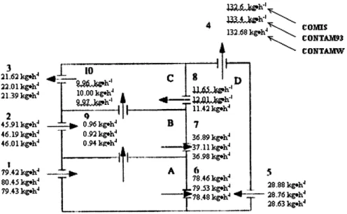
Comparison was initially conducted among COMIS, CONTAM93 (an earlier version of CONTAMW1.0), and BREEZE by other researchers. In the present study, a verification of CONTAMW1.0 is performed and the results are compared to those published. The plane view of each floor in the AIVC building and the CONTAM simulation results are shown in Figure 2.3. It also exhibits the visualized magnitudes of the mass flow rates (blue bars) and the relative pressure differences (red bars) in CONTAMW1.0. The air flows to the direction to which the blue bar points. Though highly idealized, one can easily obtain a general impression of the airflow pattern within the building. More detailed information such as zone temperature, pressure, contaminant

concentrations (if applicable) are also computed.

11

79.434 kh

28.630 kg

0.939 kg/h

L

9972

iI

Figure 2.3. Plane view of each floor of the AIVC building and CONTAM simulation results. Blue bars represent airflow rates, and red bars denote pressure.

132.68 _{gkgeh CONTAW3} CONTAUM

3

10o

-]j11.42

T

Lt78.48lA2

Figure 2.4. Simulation results - mass flow rates through the leakage paths.

The results simulated by CONTAMW1 .0 and the simulation data by COMIS and CONTAM93 published in AIVC Technical Note 51 (1999) are co-presented in Figure 2.4. In this figure, the mass flow rates are listed for each leakage opening in the order of COMIS, CONTAM93, and CONTAMW1 .0. The results obtained from the three programs are in general agreement with each other. However, the results from CONTAMW1.0 are closer to those from COMIS for this well-defined problem. For example, the airflow direction through each path simulated by different models is exactly the same, although small variations in the magnitudes (between -0. 15% and -5.2%) are detectable. The airflow rates in the figure also indicate that the results of CONTAMW1 .0 appear to be closer to those of COMIS (9 out of 10 paths), which is a little out of expectation since CONTAMi .0 and CONTAM93 are more closely related.

2.3.2 French House Case

To study ventilation and contaminant exposure, a more accurate modeling technique is required. Since the indoor airflow is quite complicated and the transport of contaminants is highly dependent on the room airflow, often a perfect mixing model is used to determine an average airflow rate and contaminant concentration level in a room. This is the basic assumption for the multizone models. A clear advantage of such model settings is its simplicity, in which the results could be validated by hand calculation for some simple problems. The major tradeoff stems quite clearly from those assumptions of instantaneous and complete mixing condition within a room, which effectively averages a value throughout the whole room.

In this section, a case study was conducted based on a house plan transcribed directly from the Mozart House from "Catalogue de Logements-Types (de Montureux 1996)" that is illustrated in Figure 2.5. The Mozart House has a floor area of 99.6 m2 and is considered to be a typical French dwelling, to which the greatest universality may be applied. The single-family house displayed in Figure 2.6 is from a CFD model without the garage, which consists of a dining/living room (36.5m2_{), a kitchen (9.5}

M2), two

childrens' bedrooms (10.9m2 _{and 11 .1m}2_{), a bathroom with a shower (3.2m}2_{), a WC (1.7}

m2

), and a master bedroom (10.1M), each containing a variety of everyday furniture.

Furniture is included as it normally affects the airflow throughout the house (Etheridge 1996) as well as changes the location of a person relative to the room (e.g. sleeping on a bed elevates the body). These factors are included to model the real world as close as possible. Figure 2.7 is the CONTAM idealization of this single-family house based on the CFD model adaptation. However, CONTAM does not have the functionality to consider the detailed furniture effect.

4.2 -Maison Mozart

4

Figure 2.5. Mozart House floor plan from Montureux 1996) used in the case study.

WC

exhaust

4

_{parents' bedroom}

table

shower bed

N

sink 4 exhaust

Figure 2.6. CFD model adaptation of the Mozart House including furniture types.

IN 9-*00@0

@@@ @000

p 0

Figure 2.7. CONTAM idealization of Mozart House based on adapted CFD model.

Considering a typical family of four, including the parents, a son, and a daughter, the house is occupied for about fifteen hours of a day. The location of each person in the house throughout the day is shown in Figure 2.8. Between 09:00-18:00h, the parents are working outside and the children are attending school, so nobody is at home during this period. Each person's activity throughout the day is shown in Table 2.1.

Occupancy Scenario 7 AVE N N N M M Er

,NMNENNO

NEENNE

_IgI,

Figure 2.8. Occupancy scenario for each person spent at home: (0) not at home (1) dining/living room (2) parents' bedroom (3) son's bedroom (4) daughter's bedroom.

Table 2.1. Daily activity of occupancy.

Hour Mother Father Son Daughter

18.00-19.00 Cooking Not home Studying Studying

19.00-21.00 Eating Dinner Eating Dinner Eating Dinner Eating Dinner

21.00-22.00 Reading Reading Studying Studying

22.00-23.00 (Smoking)

23.00-07.00 Sleeping Sleeping

07.00-07.15 Cooking Showering Sleeping Sleeping

07.15-07.30 Showering Eating Breakfast 07.45-07.45 _{Eating Breakfast}

07.45-08.00 Etn rafs

08.00-08.15 Cooking Not home Sleeping Showering

08.15-08.30 _{Showering Eating Breakfast}

08.30-09.00 Reading Eating Breakfast

Some characteristics of residential indoor environments and a variety of pollutant sources are placed within the house based on the type and level of activity. These include CO2, CO, HCHO (formaldehyde), NO2, and water vapor (H20). The characteristics of the

pollutants are listed in Table 2.2, and the strengths of the pollutant sources used in the simulations are given in Tables 2.3 and 2.4.