Publisher’s version / Version de l'éditeur:
Vous avez des questions? Nous pouvons vous aider. Pour communiquer directement avec un auteur, consultez la première page de la revue dans laquelle son article a été publié afin de trouver ses coordonnées. Si vous n’arrivez pas à les repérer, communiquez avec nous à [email protected]. Questions? Contact the NRC Publications Archive team at
[email protected]. If you wish to email the authors directly, please see the first page of the publication for their contact information.
https://publications-cnrc.canada.ca/fra/droits
L’accès à ce site Web et l’utilisation de son contenu sont assujettis aux conditions présentées dans le site LISEZ CES CONDITIONS ATTENTIVEMENT AVANT D’UTILISER CE SITE WEB.
Combustion Institute Canadian Section, 2006 Spring Technical Meeting [Proceedings], 2006
READ THESE TERMS AND CONDITIONS CAREFULLY BEFORE USING THIS WEBSITE.
https://nrc-publications.canada.ca/eng/copyright
NRC Publications Archive Record / Notice des Archives des publications du CNRC : https://nrc-publications.canada.ca/eng/view/object/?id=402ca894-3443-459b-a1fc-cfba247dc794 https://publications-cnrc.canada.ca/fra/voir/objet/?id=402ca894-3443-459b-a1fc-cfba247dc794
NRC Publications Archive
Archives des publications du CNRC
This publication could be one of several versions: author’s original, accepted manuscript or the publisher’s version. / La version de cette publication peut être l’une des suivantes : la version prépublication de l’auteur, la version acceptée du manuscrit ou la version de l’éditeur.
Access and use of this website and the material on it are subject to the Terms and Conditions set forth at
Sampling of soot emitted from lab-scale flares
Canteenwalla, P. M.; Thomson, Kevin; Smallwood, Gregory; Johnson, M. R.
SAMPLING OF SOOT EMITTED FROM LAB-SCALE FLARES
P.M. Canteenwalla1, K.A. Thomson2, G.J. Smallwood2, and M.R. Johnson11
Mechanical and Aerospace Engineering, Carleton University, Ottawa, Canada
2
Combustion Group, Institute for Chemical Process & Environmental Tech., NRC
INTRODUCTION
Flaring is a technique used extensively in the oil and gas industry to burn unwanted flammable gases. Although the emissions released through the oxidation of the gas are generally preferred over simply venting the gas to the atmosphere, flaring can create other pollution problems such as the formation of soot. Fine soot particles (less than 2.5 µm) have been linked to serious health effects such as cancer and heart disease in humans and animals [1]. To date little attention has been focused on this problem despite federal requirements for industry to quantify and report particulate matter (PM) emissions (i.e. soot) through the National Pollutant Release Inventory. Field measurements of soot emissions from flares are difficult for several reasons: the ambient conditions are constantly changing, the emissions can be rapidly dispersed in the atmosphere leading to poor sampling, and there is large site-to-site variation of flares so measurements at a single site are not representative of every flare. In light of these difficulties, it was decided to create a scale flare to allow emission measurements in a controlled environment. The lab-scale flare is able to operate under a wide range of conditions to simulate field conditions. The experiments will investigate effects of varying fuel composition, fuel flow rate, and flare diameter on soot emissions.
However, there are challenges associated with simulating a flare under laboratory conditions. The dilution ratio, relative humidity, residence time, and temperature of the sample exhaust can all lead to a significant change in the soot emissions [2, 3]. These effects need to be investigated to ensure that measured emissions at the sample location can be accurately related to actual emissions from the flame. Only then can these data be used to estimate soot emission from flares under field conditions. This paper outlines a methodology for sampling soot emissions from the lab-scale flare to determine the mass emission rate of soot per mass of fuel burned within calculated uncertainties. Also considered is the effect of dilution air temperature on the soot particle size distribution.
The end goal of this research is to develop an experimentally based model to predict PM emissions from flares used in industry using soot emissions data from lab-scale flares. Such a model will help industry to meet its federally mandated reporting requirements while providing industry a framework for emissions reduction.
EXPERIMENTAL SETUP
The main goal in the design of the experimental setup was to create a system that could operate under a wide range of conditions, which could simulate field conditions.
Lab-scale Flare
The lab-scale flare consists of five main components; the diffuser, settling chamber, converging nozzle, turbulence generating grids, and burner exit (Figure 1). The multi-component fuel mixture enters the diffuser which is filled with 5 mm glass beads to breakup the incoming fuel jet and to help uniformly distribute the flow. The flow then enters a settling chamber containing three equally spaced fine mesh screens followed by a converging nozzle which creates a uniform top-hat velocity profile upstream of the turbulence generating grid. The turbulence generating
grid is placed 3 to 5 diameters from the burner exit and is used to produce a turbulent velocity profile at the burner exit which is characteristic of the fully developed pipe turbulence expected in a full-size flare. Different nozzles and turbulence grids can be chosen to accommodate flare exit tubes up to 76.2 mm in diameter.
Settling Chamber Diffuser Nozzle Turbulence Generating Grid Burner Exit Settling Chamber Diffuser Nozzle Turbulence Generating Grid Burner Exit
Figure 1: Schematic of lab-scale flare Figure 2: Sampling system schematic
Sampling System
The lab-scale flare is situated inside an aluminum cage (1.5 x 1.5 x 2.5 m high) as shown in Fig. 2. The exhaust is discharged into an insulated 152 mm diameter duct. A 9.5 mm diameter probe samples at a single point within the duct. A fully mixed exhaust is required to ensure that a single point sample is representative of the entire duct. A variable iris damper is used to create a flow obstruction within the duct to promote mixing. The sample is drawn through a heated sample line and analyzed by a scanning mobility particle sizer (SMPS, DMA Model 3080, CPC Model 3081, TSI) which measures the number concentrations and electric mobility diameter of particles ranging from 15 nm to 673 nm during a 120 second scan time. A laser-induced incandescence (LII) system is used to measure the soot volume fraction. The dilution ratio is controlled by a variable speed fan and measured using an O2 Analyzer (Siemens, OXYMAT 6).
At the time of submission of this paper, the LII and O2 Analyzer were still being commissioned.
SOOT YIELD AND ERROR ANALYSIS
For industry and regulators, source emissions of soot are best quantified on a mass of soot per mass of fuel basis known as soot yield (Ys). However, the LII gives a measurement of soot volume fraction (fv) which is a volume of soot per volume of sample air. The following equations outline a sampling protocol for determining Ys from measured LII data.
The soot volume fraction, fv, in a sample drawn from the exhaust duct and measured using LII is defined as, fv = Vsoot /Vsample, where Vsoot is the volume of soot within the optical sample volume, Vsample. For iso-kinetic sampling from fully mixed conditions in the exhaust duct, this is equivalent to fv = Qsoot / Qduct where Qsoot and Qduct are the volume flow rates of soot and gases through the exhaust duct. Since the soot particles are demonstrated to be extremely small (<1μm), the requirement for iso-kinetic sampling is not at all critical as the particles will readily track the flow into the sample probe. Although the sample is drawn through a heated line, if the temperature at the LII measurement location differs from the temperature at the sample point in
the duct, the change in gas volume of the sample must also be considered. Assuming ideal gas behaviour, the measured soot volume fraction is related to conditions in the duct via Eq. (1).
⎟⎟ ⎠ ⎞ ⎜⎜ ⎝ ⎛ = = duct sample sample v duct soot duct v T T f Q Q f , , (1)
If we assume that all of the measured soot originates from the flare, then if the volume flow rate in the duct can be determined, the mass emission rate of soot can be calculated as,
duct duct v soot soot f Q m& =ρ ⋅ , ⋅ (2)
Since the dilution ratio (DR) of combustion products in the duct needs to be monitored as part of establishing a reliable soot sampling protocol [2,3], one approach to determining Qduct can be found by using the measured dilution ratio and calculated flow of combustion products from the flare. By measuring oxygen concentrations in the exhaust duct and in the ambient room air, the dilution ratio can be determined as follows:
[ ]
[ ]
[ ]
products air dilution sample air room air room Q Q O O O DR = − = 2 2 2 (3) The ambient-temperature flow rate of combustion products, Qproducts, can be calculated by balancing the stoichiometric hydrocarbon combustion reaction equations assuming complete combustion. The potential uncertainty associated with assuming complete combustion is insignificant as shown below. The actual volume flow rate of mixed dilution air and combustion products through the exhaust duct can then be calculated as follows:(
)
[
]
ambient duct products products duct T T Q DR Q Q = ⋅ + (4)Combining equations (1-4), the mass flow rate of soot from the flare can then be calculated as,
(
)
, 1 ,
sample soot soot v sample products
ambient T m f Q DR T ρ = ⋅ ⋅ + & (5)
which relates to the soot yield as,
(
)
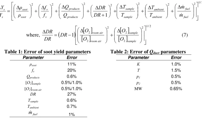
ambient fuel sample products sample v soot fuel soot s T m T DR Q f m m Y ⋅ ⋅ + ⋅ ⋅ ⋅ = = & & & ρ , 1 (6)The estimated uncertainty in soot yield for this approach can be calculated from Eq. (7). Table 1 contains approximate values of the expected error for the various parameters. There are several different values published in the literature for ρsoot which will be assumed to have a value of 1.8 ±
0.2 kg/m3. The error in fv is mainly due to the uncertainty in optical properties of soot. The repeatability of LII is quite good with an error of less than 5%. Error in Qproducts would result from an incorrect estimation of the combustion efficiency. The error listed in Table 1 would result from a soot yield calculation made assuming complete combustion (100%) when the actual combustion efficiency was 95%. The temperature error was calculated based on a thermocouple with an accuracy of ± 2 K on temperatures of 293 K and 333 K for Tambient and Tduct, respectively. The error in Ys is extremely sensitive to the DR and oxygen concentrations. The two values given for the DR error correspond to an oxygen concentration error of 0.5% and 1%. Combined with the other parameters, the total error in Ys is 26% and 34% for an oxygen concentration error of 0.5% and 1%, respectively.
2 / 1 2 2 2 2 2 2 2 1 ⎥⎥ ⎦ ⎤ ⎟ ⎟ ⎠ ⎞ ⎜ ⎜ ⎝ ⎛ Δ + ⎟⎟ ⎠ ⎞ ⎜⎜ ⎝ ⎛ Δ + ⎟ ⎟ ⎠ ⎞ ⎜ ⎜ ⎝ ⎛ Δ ⎢ ⎢ ⎣ ⎡ + ⎟ ⎠ ⎞ ⎜ ⎝ ⎛ + Δ + ⎟ ⎟ ⎠ ⎞ ⎜ ⎜ ⎝ ⎛ Δ + ⎟⎟ ⎠ ⎞ ⎜⎜ ⎝ ⎛ Δ + ⎟⎟ ⎠ ⎞ ⎜⎜ ⎝ ⎛ Δ = Δ fuel fuel ambient ambient sample sample products products v v soot soot s s m m T T T T DR DR Q Q f f ρ ρ Y Y & & where,
(
)
[ ]
[ ]
[ ]
[ ]
2 / 1 2 2 2 2 2 2 1 ⎥ ⎥ ⎦ ⎤ ⎢ ⎢ ⎣ ⎡ ⎟ ⎟ ⎠ ⎞ ⎜ ⎜ ⎝ ⎛ Δ + ⎟ ⎟ ⎠ ⎞ ⎜ ⎜ ⎝ ⎛ Δ − = Δ sample sample air room air room O O O O DR DR DR (7)Table 1: Error of soot yield parameters Parameter Error ρsoot 11% fv 20% Qproducts 0.6% [O2]sample 0.5%/1.0% [O2]room air 0.5%/1.0% DR 27% Tsample 0.6% Tambient 0.7% fuel m& 1%
Table 2: Error of Qduct parameters
Parameter Error K 1.0% T 1.5% p1 0.5% p2 0.5% MW 0.65%
An alternative approach to solving Eq. (2) is to measure Qduct directly. This could be accomplished by numerous methods (e.g. orifice flowmeter, turbine meter). The following shows an error analysis using an orifice flowmeter. In this case, Qduct is given by,
2 1 2 p p g KA Q duct duct = ρ − (8)
where K is a flow coefficient, A is the duct cross-sectional area, ρduct is the density of the mixed gases in the duct, and p is the static pressure. Determination of ρduct requires knowledge of the gas composition and temperature which will vary with the DR of combustion products and entrained room air. However, assuming ideal gas behavior and complete combustion of a methane based fuel, the molecular weight of the mixed gases in the duct will only vary from 28.557 to 28.744 (0.65 %) as DR varies from 5 to 100. An uncertainty estimate for Qduct can be calculated with Eq. (9) where the density of the exhaust gases is related to the temperature (T) and pressure (p), and molecular weight (MW) through the ideal gas equation of state.
2 2 2 2 1 1 2 2 2 4 1 2 1 4 1 4 1 ⎟⎟ ⎠ ⎞ ⎜⎜ ⎝ ⎛ Δ + ⎟⎟ ⎠ ⎞ ⎜⎜ ⎝ ⎛ Δ + ⎟ ⎠ ⎞ ⎜ ⎝ ⎛ Δ + ⎟ ⎠ ⎞ ⎜ ⎝ ⎛ Δ + ⎟ ⎠ ⎞ ⎜ ⎝ ⎛ Δ = Δ p p p p MW MW T T K K Q Q duct duct (9)
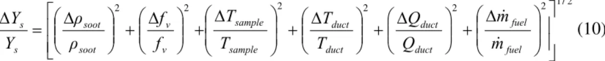
The error for K was found from Husain for an orifice that conforms to standard mechanical tolerances and installation [4]. With the errors listed in Table 2, the uncertainty in a measurement of Qduct would be approximately 2.1 %. This is compared to an uncertainty of 13% by calculating Qduct with Eq.(4) and assuming 0.5% error on the oxygen concentrations. Assuming uncertainty values from Table 1 for the remaining terms in Eq. (2), the resulting uncertainty in Ys for a calculation involving a direct measurement of Qduct can be calculated from Eq. (10) and is estimated at 23 %. This uncertainty is actually less than that for the dilution ratio method. However, it is noted that as DR is reduced the uncertainty in the O2 method decreases
2 / 1 2 2 2 2 2 2 ⎥ ⎥ ⎦ ⎤ ⎟ ⎟ ⎠ ⎞ ⎜ ⎜ ⎝ ⎛ Δ + ⎟⎟ ⎠ ⎞ ⎜⎜ ⎝ ⎛ Δ + ⎟⎟ ⎠ ⎞ ⎜⎜ ⎝ ⎛ Δ + ⎟ ⎟ ⎠ ⎞ ⎜ ⎜ ⎝ ⎛ Δ ⎢ ⎢ ⎣ ⎡ + ⎟⎟ ⎠ ⎞ ⎜⎜ ⎝ ⎛ Δ + ⎟⎟ ⎠ ⎞ ⎜⎜ ⎝ ⎛ Δ = Δ fuel fuel duct duct duct duct sample sample v v soot soot s s m m Q Q T T T T f f ρ ρ Y Y & & (10)
Since the end goal of this project is to measure the total mass of soot emissions it is important to avoid particle deposition wherever possible as this will increase the soot yield error. However, it may not always be possible to control the deposition mechanism; for example, in the case of the SMPS it is not possible to heat its internal lines. Brockmann [5] has outlined numerous calculations to determine the transport efficiency of particles in sample lines. Therefore, in the cases where the deposition mechanism cannot be controlled, an estimate of losses can be made through these calculations. Listed below are equations to calculate thermophoretic losses (ηth) given by Brockmann and line losses (ηline) from Hurley [6]. These equations are given in terms of efficiency which is a ratio of particles leaving the line to those entering the line. More equations for losses in bends in the sample line and obstructions can be found in Brockmann [5].
Line Losses Thermophoretic Losses in Turbulent Flow
(
)
⎟ ⎠ ⎞ ⎜ ⎝ ⎛− − + − = dV L E V E line exp 1.05 4 2.27 4 η ⎥ ⎦ ⎤ ⎢ ⎣ ⎡ − = Q V L d th th π η expwhere: Vth = thermophoretic velocity
V = sample line velocity (18.1 m/s) d = sample line diameter (0.15 m) L = sample line length (4 m)
Q = sample line volumetric flow rate (0.33 m3/s) kg = thermal conductivity of gas (0.024 W/m·K)
kp = thermal conductivity of particle (1 W/m·K)
P = pressure (101325 Pa)
∇T = temperature gradient (130 K/m)
For particles in the continuum regime,
(
)
⎟ ⎟ ⎠ ⎞ ⎜ ⎜ ⎝ ⎛ + ∇ = p g g p g th k k P T k k k V 2 1 5 / 2A rough estimate of losses can be made from the current setup conditions which are given above in parentheses. The temperature gradient is estimated by taking a mean gas temperature of 333 K and an estimated duct wall temperature of 323 K. With these values ηline and ηth are both calculated to be approximately 99%.
RESULTS AND DISCUSSION
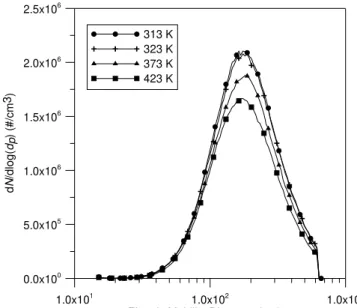
The effect of dilution air temperature on the soot particle size distribution (Figure 3) was investigated by varying the temperature between 313 K – 423 K on the sample line which draws exhaust from the duct to the SMPS. The exhaust temperature in the duct at the sampling point was 323 K. Ethylene was used at a flow rate of 8.5 LPM for this experiment.
Figure 3 shows the soot particle size distribution results from the SMPS which are presented as dN/dlog(Dp) where N is the number concentration and Dp is the electric mobility diameter. The results show that the number concentration decreased with increasing dilution air temperature while the mean diameter stayed approximately constant at 200 nm. Both Chang [2] and Kittelson [3] report that the dilution air temperature had an effect on the nucleation rate and growth of ultrafine particles (Dp < 100 nm). However, an effect on nucleation rate and growth would cause a shift in the mean diameter which cannot be seen in Figure 3.
The number density decrease shown in Figure 3 could be occurring due to thermophoresis downstream of the heated sample line once the exhaust entered the short length of inlet piping of
the SMPS which was essentially at room temperature. In this case, the increase in sample line temperature would cause an increased temperature gradient between the soot particles and the SMPS inlet piping which could increase thermophoretic deposition.
1.0x101
1.0x10²
1.0x10³
Electric Mobility Diameter (nm) 0.0x100 5.0x10⁵ 1.0x10⁶ 1.5x10⁶ 2.0x10⁶ 2.5x10⁶ d N /d lo g( dp ) ( #/ cm 3) 313 K 323 K 373 K 423 K
Figure 3: Effect of temperature on soot particle size distribution
CONCLUSION
A method to quantify soot yield from lab-scale flares has been developed. Analysis has shown that directly measuring flow rate in the exhaust produces less uncertainty in measured soot yield than an approach based on measuring the dilution ratio of combustion products using an O2
analyzer. Calculations also suggest that for the current duct system, thermophoretic losses are effectively minimized under normal operating conditions and can be controlled by minimizing the temperature gradient between the soot particles and the sample line walls. Preliminary data from SMPS measurements show the dilution air temperature does not have an effect on the nucleation rate or growth of soot particles at the duct temperatures expected in the sampling system. However, at higher temperatures, thermophoretic losses in the inlet piping of the SMPS may become significant.
ACKNOWLEDGEMENTS
This project is supported by the Canadian Association of Petroleum Producers (CAPP) and Environment Canada (Project Manager, Michael Layer).
REFERENCES
[1] C. Arden et al. “Lung Cancer, cardiopulmonary mortality, and long-term exposure to fine particulate air pollution,” Journal of the American Medical Association 287, 1132-1141 (2002).
[2] O. Chang et al. “Measurement of Ultrafine Particle Size Distributions from Coal, Oil, and Gas Fired Stationary Combustion Sources,” Journal of the Air & Waste Management Association 54, 1494-1505 (2004).
[3] D. Kittelson et al. “The Influence of Dilution Conditions on Diesel Exhaust Particle Size Distribution Measurements,” SAE Technical Paper Series 01-1142 (1999).
[4] Z.D. Husain, “Theoretical Uncertainty of Orifice Flow Measurement” Daniel Flow Prod. Inc., Houston, (1995). [5] J.E. Brockmann, P. Baron ed., K.Willeke ed., Aerosol Measurement – Chapter 8: Sampling and Transport of
Aerosols, 2nd Ed., U.S.A., John Wiley and Sons (2001).
[6] C.D. Hurley, “Smoke Measurements Inside a Gas Turbine Combustor,” AIAA/SAE/ASME /ASEE 29th Joint Propulsion Conference and Exhibit Monterey, CA. (1993)