A 3-D tunnel correction panel method for swept tapered airfoils with separation

A 3-D TUNNEL CORRECTION PANEL METHOD FOR SWEPT TAPERED AIRFOILS WITH SEPARATION

by

John Henry Burns

B.S.A.E., University of Colorado Boulder (1985)

SUBMITTED TO THE DEPARTMENT OF AERONAUTICS AND ASTRONAUTICS

IN PARTIAL FULFILLMENT OF THE REQUIREMENTS FOR THE DEGREE OF

MASTER OF SCIENCE IN

AERONAUTICS AND ASTRONAUTICS

at the

MASSACHUSETTS INSTITUTE OF TECHNOLOGY January 1988

0

Massachusetts Institute of Technology 1988 Signature of Author ._

--Department of Aeronautical and Astronautical Engineering January 29, 1988 Certified by Accepted by Dr. Ju son R. Baron Thes s SuperVisor Dr. Harold Y. Wachman Chairman, Departmental Graduate Committee

MASSACHUSS INSMTJt FEB 0 4 198!) LIBRARIES %WDRAWN M.I.T. AeLIBARES

Aero

A 3-D TUNNEL CORRECTION PANEL METHOD FOR SWEPT TAPERED AIRFOILS WITH SEPARATION

by

JOHN HENRY BURNS

Submitted to the Department of Aeronautics and Astronautics on January 29, 1988 in partial fulfillment of the requirements

for the degree of

Master of Science in Aeronautics and Astronautics

ABSTRACT

Wind tunnel walls, by their presence, alter air flow around the model and thus the data gathered. Classical methods of wind tunnel wall corrections are of questionable accuracy for extreme test conditions (i.e. high angle of attack with separation). A computational method has been developed to calculate wind tunnel wall interference for wings of arbitrary sweep and taper. Additional wings may be present to represent a horizontal tail, canard, or multiple wings. The closed test section tunnel is of arbitrary eccentricity and a vertical wing with a ground board can be simulated. A three dimensional vortex panel method is used to model the wing and its wake. A two dimensional boundary layer analysis is used to find the separation locus. The separation locus and wake shape are found by iteration.

The results show proper convergence trends for a range of sweep, dihedral, taper, and aspect ratio. The data shows proper behavior for variations of the wing planform and tunnel eccentricity.

Thesis Supervisor: Dr. Judson R. Baron

3

Acknowledgements

Thanks to all of my friends who have helped make my stay at M.I.T. both productive and pleasant, with special thanks to Jon Mishler. Thank you, Tim Gilbert, Susan Tucker, Dave Kikorian, Don Robinson, and Octavio Marenzi for your help with the figures.

At the Wright Brothers Facility I have had the pleasure of working with many fine graduate students, all of whom have influenced myself and my work: John Busch, Charles Boccadoro, Tim Gilbert (my favorite civil engineer), Don Robinson, and Mike D'Angelo.

I wish to thank Frank Durgin, assistant director of the Wright Brothers Facility, for his insights into all aspects of wind tunnel testing.

I wish to express my sincere appreciation to Professor Judson R. Baron, my advisor, for his continuous assistance and availability during my stay at M.I.T.

5 Table of Contents Chapter Pare Abstract --- 2 Dedication --- 3 Acknowledgements --- 4 Table of Contents --- 5 List of Figures --- 6 Nomenclature --- 9 1 Introduction --- 12

2 Qualitative Description and Modeling of Flow ---- 19

3 Potential Flow Equation --- 24

Theoretical Foundation of Panel Methods --- 26

4 Calculation of Potential Flow --- 31

Panel Formulation --- 32

Paneling --- 33

Calculation of Induced Velocities --- 38

Matrix Equation --- 48

Matrix Solution Procedure --- 55

5 Boundary Layer Analysis --- 57

Laminar Boundary Layer --- 59

Transition --- 63

Turbulent Boundary Layer --- 64

6 Discussion of Results --- 74

2-D Attached Flow --- 74

3-D Attached Flow --- 78

Separation --- 88

7 Conclusions and Recommendations --- 98

Appendix A Integration of Selected Velocity Functions --- 101

B Code Lfly --- 109 Flow Chart --- 110 Sample Input --- 111 Sample Output --- 113 Code Listing --- 116 Figures --- 231 References --- 281

List of Ficures

Page

2-1 Flow regions surrounding an airfoil --- 232

4-1 Panel planform --- 233

4-2 Wing paneling and coordinate system --- 234

4-3 Tunnel cross section --- 235

4-4 Tunnel nomenclature and coordinate system ---- 236

4-5 Panel vorticity distribution --- 237

4-6 Vortex filament coordinate system --- 238

4-7 Vortex filament sections --- 239

6-1 Lift versus inverse number of wing panels along chord ---- --- 240

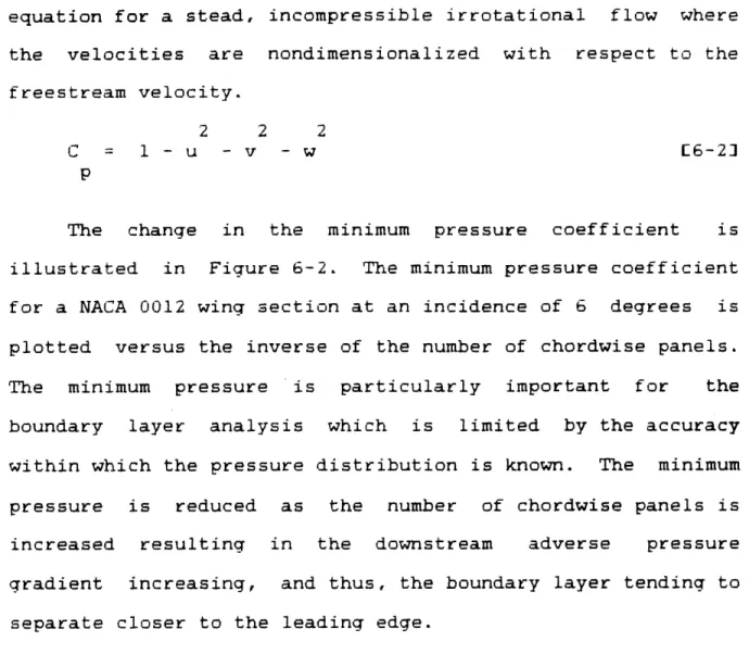
6-2 Negative peak pressure coefficient versus inverse number of wing panels along chord 241 6-3 Thin airfoil 2-D biplane and wake geometry --- 242

6-4 2-D biplane lift versus inverse number of wing panels along chord --- 243

6-5 Lift coefficient versus inverse number of wing panels along chord --- 244

6-6 Lift coefficient ratio versus inverse number of wing panels along chord --- 245

6-7 Lift coefficient versus inverse number of wing semi-span panels --- 246

6-8 Lift coefficient ratio versus inverse number of wing semi-span panels --- 247

6-9 Lift coefficient ratio versus number of panels along tunnel length --- 248

6-10 Lift coefficient ratio versus number of circumferential tunnel panels --- 249

7

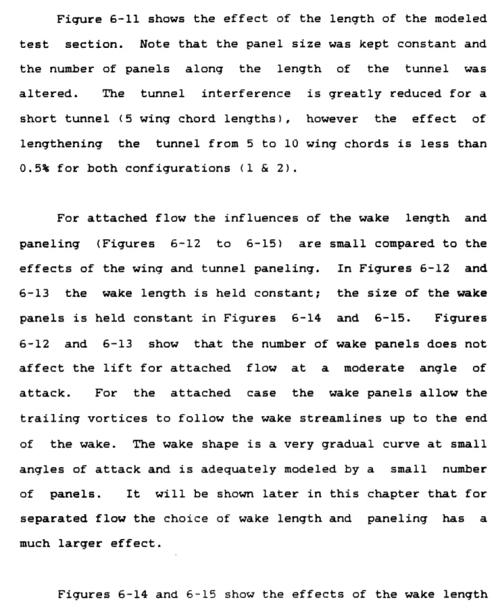
6-12 Lift coefficient versus number of wing wake

panels in downstream direction 251

6-13 Lift coefficient ratio versus number of wing

wake panels in downstream direction --- 252 6-14 Lift coefficient versus wake length for

attached flow --- 253

6-15 Lift coefficient ratio versus wake length for

attached flow --- 254 6-16 Lift coefficient versus wing dihedral angle -- 255 6-17 Lift coefficient ratio versus wing dihedral

angle --- 256 6-18 Lift coefficient versus sweep angle --- 257 6-19 Lift coefficient ratio versus sweep angle ---- 258 6-20 Lift coefficient versus wing taper ratio --- 259 6-21 Lift coefficient ratio versus wing taper ratio 260 6-22 Lift coefficient versus wing aspect ratio ---- 261 6-23 Lift coefficient ratio versus wing aspect

ratio --- 262 6-24 Lift coefficient ratio versus span ratio (B/b) 263 6-25 Lift coefficient ratio versus tunnel

eccentricity (span ratio constant) --- 264 6-26 Lift coefficient ratio versus tunnel

eccentricity (tunnel area constant) --- 265 6-27 Lift coefficient ratio versus round board

height --- 266 6-28 Spanwise lift distribution versus wing aspect

ratio --- 267 6-29 Spanwise circulation distribution versus wing

sweep angle --- 268

6-30 Spanwise circulation distribution versus wing

taper ratio --- 269 6-31 Coefficient of lift versus wake panel density 270

6-33 Pressure distribution of wing 4 at alpha = 2.8 degrees --- 272 6-34 Pressure distribution of wing 4 at alpha = 7.4

degrees --- 273 6-35 Pressure distribution of wing 4 at alpha =

13.8 degrees --- 274 6-36 Pressure distribution of wing 4 at alpha =

17.9 degrees --- 275 6-37 Pressure distribution of wing 4 (nc = 30) at

alpha = 17.9 degrees --- 276 6-38 Initial and converged wake geometry at alpha =

13.8 degrees --- 277 6-39 Convergence history for wing 4 at alpha = 13.8

degrees --- 278 6-40 W:ing pressure distribution in tunnel ---- 279

Wing pressure distribution in free air

9 NOMENCLATURE [A] AR B {B) b b c C' C1 CL CLfa CLt Fl,F2,G1,G2 H Ht Coefficient matrix Win aspect ratio Tunnel semi-width

Right hand side column matrix Wing span

Panel span

Wing root chord Panel chord

Coefficient of lift/unit span Coefficient of lift

Coefficient of lift in free air Coefficient of lift in tunnel

Induced velocity subfunctions Boundary layer shape parameter Tunnel semi-heicht

ith chordwise panel ith spanwise panel

Number panels along chord

Number of panels across semi-span inc ins nc ns p P Re Re Static pressure Total pressure

Reynolds number based on wing root chord Reynolds number based on distance x

Reynolds number based on boundary layer momentum thickness Wing semi-span S U ,V' ,W Cu],£v] ,[w]

[u'

]

,v'

]

,w'

]

V V' Vi WL

X}

x

' ,

y

,

z '

r

A

'/4

0

AL Wing area

Velocity components in global frame Velocity components in panel frame

Induced velocity matrices - global frame

Induced velocity matrices - local panel frame Velocity vector in global coordinates

Velocity vector in panel coordinates Free stream velocity

Wake length

Column matrix of panel strengths Global coordinates

Panel coordinates Angle of incidence Dihedral angle

Circulation / unit length Circulation

Sweep angle of wing 1/4 chord Panel sweep angle

Tangent of panel sweep angle Velocity potential

Perturbation velocity potential Boundary layer momentum thickness Coefficient of dynamic viscosity Coefficient of kinematic viscosity

Ree

11

CHAPTER 1

INTRODUCTION

The historic flight of the Wriaht brothers in 1903 demonstrated the value of wind tunnel testing, which was used methodically to design their airfoils. The fact that Rockwell spent 46,500 hours testing models of the space shuttle in various wind tunnels during the design phase of that program CWhitnah and Hillje (1)] shows the ever continuing need for wind tunnel testing. It is still impractical to solve the full Navier-Stokes equations for a flight vehicle either analytically or numerically. Analytical solutions exist only for very special boundary conditions and the computational effort needed for the direct numerical modeling of turbulent shear layers at flight Reynolds numbers is beyond the ability of any computing machines for the forseeable future. Wind tunnel testing remains crucial for the successful design and optimization of flight vehicles due to its ability to directly model the physics without simplifying assumptions, while encompassing all scales of motion and time.

While the solution by direct analogy is complete, it is only as accurate as the analogy. The similarity conditions for a low speed test in which gravitational forces and flexibility are negligible requires the matching of model

13

geometry, Mach number, and Reynolds number. The matching of both Mach number and Reynolds number is difficult to achieve unless either the model is full-sized or a custom working fluid is used in the tunnel. If sea level air is used in a tunnel the largest model possible allows for the closest match of both Reynolds number and Mach number.

While the physics of a wind tunnel test may be correct, the boundary conditions match only in the limit of an infinitely large tunnel diameter compared to a representative length of the model. The boundary conditions for free flight are a uniform flow field at infinity, which is equivalent to an unaltered streamtube at infinity, but not to the tunnel conditions of an unaltered streamtube at the tunnel walls. The effects of such flow field constraints is collectively known as wind tunnel wall interference. The wall interference alters the aerodynamic behavior of the model compared to free flight conditions. Thus, the effects of the wall interference must be accounted for before the data is representative of free air conditions.

If an exact calculation of the wall interference followed from solving the complete fluid governing equations for a model both in free air and in the tunnel, the ability to completely solve the governing equations would limit the need for wind tunnel testing. However, wind tunnel verification

would still be necessary to have the confidence to build a prototype. The wind tunnel analogy remains the only "method" for solving the flow field completely.

Classical methods of wind tunnel wall corrections approximate the wing, wake, and trailing vorticity using flow singularities. Images of the singularity distribution representing the wing, wake, and trailing vorticity are arranged in a configuration such that the wind tunnel wall boundary conditions are implicitly enforced. The interference flow field of the tunnel is represented by the image singularities. This interference can be interpreted as a variation in the flow direction, speed, and curvature. However, in the classical approach, at high angles of attack, wake curvature and flow separation are ignored and therefore are questionable under such conditions. Rae and Pope (2) present a detailed description of the effects of wall interference and classical correction methods. Joppa (3) provides a short history of the development of wall corrections including Prandtl and Glauertis work. Classical wall corrections are linear because the strength of the image vortices are directly proportional to the lift of the model.

The major effects of wall interference on a typical wing flow for a closed wind tunnel are summarized as:

15

1) An acceleration of the flow around the model known as "solid blockage" is due to the volume of the model and the constraint of the walls.

2) An acceleration of the flow around the low speed wake known as "wake blockage" is due to the conservation of mass flow within the tunnel walls

3) An alteration of the free air spanwise variation of angle of attack significant for wings that span more than 80% of the tunnel, causing the tips to stall earlier than in free air.

4) A change of flow curvature about the wing increasing the lift and moment.

5) The normal downwash at the wing is changed, causing an increased lift and decreased drag.

More recently other methods of wind tunnel wall interference corrections have been developed which use computers to carry out calculations too long and tedious to be reliably calculated by hand in a reasonable amount of time. Methods of calculating the wall interference flow based on a "wall pressure signature" 4,5) require the use of extensive wall pressure data. They are similar to higher order classical techniques (with the additional information of the pressures at the walls) in that the interference flow of the tunnel is calculated and utilized to calculate the corrections.

The most elegant approach attempts to completely remove the wind tunnel wall interference instead of correcting for it. The adaptive wall method (6,7,8) alters the streamtube defined by the wind tunnel walls by matching it to the

corresponding streamtube in free air. Practical limits in the adjustments may prevent the complete elimination of such interference, but the technique is used to minimize wall interference to some extent. The method requires extensive pressure sensing and the iterative method of adjusting the walls requires solving for the pressures of the free air streamtube. The expense of an automated system that adjusts the wind tunnel walls prevents this idea from being applicable to most tunnels.

Hess and Smith (9) developed a pioneering panel method for calculating the potential flow around arbitrary bodies, which was published in 1966. Since then many investigaters (10,11,12,13) have introduced other panel methods to calculate the flow over a wing. The wing is represented by distributed panels, where each panel is a singularity with a strength determined such that the tangential flow condition and Kutta condition are enforced. A natural extension of classical methods of wall corrections, given the digital computer to carry out the calculations, is the use of multiple singularities to model the wing in greater detail, and either the use of images to implicitly model the walls or the use of singularities to directly model the tunnel surfaces. Thus, vortex lattice (14) and panel (15,16,17) methods for wall corrections are the descendants of classical methods.

17

Olechowski (14) developed a vortex lattice method for calculating wall interference including the effects of separation. The method requires the separation locus of the wing to be determined in the wind tunnel test. The separation locus for the free air calculation is assumed to be the same as the separation locus in the tunnel. This assumption is questionable because the wall interference may affect the

separation locus on the wing.

Tennison (15) developed a distributed vorticity panel method which included a boundary layer analysis routine to find the separation locus. The fact that the wall

interference may alter the separation locus of the model compared to free flight conditions is accounted for by his approach. However, the modeling used an open wake with

straight parallel boundaries.

Both Olechowski and Tennison developed their methods at the Wright Brothers Facility at M.I.T. The predominance of complicated wing configuration designs makes those methods which are limited to a single rectangular wing without dihedral unapplicable to most tests. At present the only aircraft with wings that are close to retangular planform are small private airplanes such as a Piper Cub, and even those planes typically have a small amount of sweep, taper and dihedral. Thus, the features needed include the use of

multiple wings of arbitrary sweep, taper and dihedral. This work was undertaken at the Wright Brother Facility to provide a design method which would be applicable to wind tunnel tests of wings that are somewhat more represenative of "real" airplanes.

The following is a formulation of a 3-D wall interference method that uses vortex panels to represent the model, walls, and free shear layers. Spanwise stations are treated with a 2-D boundary layer analysis to determine a separation location for each strip of the wing. The wake is adjusted independently at each spanwise station until the upper and lower edges of the wake lie along streamlines. There is no constraint on the shape of either the upper or lower wake. On the final iteration both the separation locus on the wing and the wake shape have converged. The tunnel is excluded when solving for the model in free air. This is equivalent to placing the model in a tunnel of infinite diameter compared to a representative length of the model. The effect of the displacement thickness of the boundary layers is not modeled at this time. The wake consists of unconnected strips of the same dihedral as the wing, and the rollup of the trailing vortices is not modeled.

19

CHAPTER 2

QUALITATIVE DESCRIPTION AND MODELING OF FLOW OVER A WING

Figure 2-1 illustrates the physical problem of separated flow. The ideal modeling is described later in this chapter and is obtained from the technique explained more fully in Chapter 4. Before examining the separated case shown in Figure 2-1 a brief explanation of the attached case is in order.

The boundary layers in the so-called attached case in fact effectively separate from the airfoil at the upper and lower trailing edges, resulting in an absence of a separated region over the airfoil itself, and confining the viscous wake region to the combined thickness of the trailing edge and both boundary layers. From Helmholtz's vortex theorem a two dimensional wing creates no new net vorticity in a steady flow. Therefore, the boundary layer vorticity that is shed from the upper and lower trailing edges must be equal in magnitude and opposite in orientation. This corresponds to a Kutta condition of no net vorticity at the trailing edge. The 3 dimensional case requires a modification of the Kutta condition modeling for attached flow. This modeling problem, its solution, and the underlying cause are discussed in

The comparative advantage of panel methods over classical methods as a basis for wall interference effects originates from an increased accuracy of the wing modeling, and would be lost if the separation was not included when present. There are three distinct types of separation: bubble, leading edge, and trailing edge. Bubble separation usually occurs when a laminar boundary layer separates from the surface of the airfoil. The resulting thin free shear layer changes from laminar to turbulent, due to the instability of the thin free shear layer, and the turbulent thin free shear layer reattaches to the airfoil as a turbulent boundary layer. The latter is robust because the turbulent mixing brings high energy fluid into the boundary layer, allowing it to withstand a relatively greater adverse pressure gradient before separating than does a laminar boundary layer. Bubble separation is divided into long and short categories depending upon the length of the separated region. In the present modeling, separation is assumed to be of the short bubble variety for laminar situations. The separation bubble is modeled as being of negligible length and any thickening of the boundary layer is neglected. When the angle of attack is gradually increased the boundary layer eventually leaves the airfoil surface and jumps suddenly to near the leading edge. In the case of trailing edge separation, the point of separation moves smoothly forward from the upper trailing edge as the angle of attack increases past that angle for which

21

attached flow can be maintained. The maximum angle of fully attached flow varies with the wing section, Reynolds number, surface roughness, and free stream turbulence. An angle of approximately 8 degrees (18) represents the maximum angle of fully attached flow for a NACA 0012 airfoil at a Reynolds number between 3 and 9 million. This airfoil is subject to the trailing edge type of separation.

The steady separated flow over a wing at high Reynolds numbers and low Mach numbers consists of four distinct regions as shown in Figure 2-1. An examination of each region and their interactions suggests which physically reasonable assumptions are needed to make the problem tractable, and also suggests a technique for modeling the separated flow over a wing.

Initially irrotational upstream of the airfoil, the flow remains irrotational in the essentially potential flow region (exterior to all shear layers and wakes) because everywhere in that region the shear is essentially negligible. The flow in such a potential region interacts with its surroundings only through pressure forces, and has been modeled here by a Laplace equation which assumes it is both irrotational and incompressible (low Mach number).

surface of the airfoil and the outer potential flow. The shear at the inner solid boundary generates large viscous forces and vorticity which is confined to the boundary layer. The displacement thickness of the boundary layer has not been added to the thickness of the wincr. A number of investigators (19) have developed methods that accurately predict the behavior of boundary layer parameters from the pressure distribution along the layer's outer boundary adjacent to the potential flow region. The boundary layer has been modeled here using Thwaites' (20) laminar analysis, a modification of Michel's transition criteria (19) and Stratford's (22) turbulent separation criteria.

A thin free shear layer, if present, is fed by a separating boundary layer and defines the boundary between essentially two inviscid regions, such as for example, an outer potential flow and an inner separated region. Shear and viscous forces are relatively moderate in the thin shear layer when compared with those in a boundary layer. The thin free shear layer is modeled as a discontinuity surface by a continuation of the surface vortex panels from which it extends. At the trailing edge of an airfoil with upper surface separation the boundary layer from the lower surface leaves to form a second thin free shear layer. The thin free shear layers then follow the streamlines of the flow and are essentially slip surfaces across which a jump in tangential

23

velocity exists. The vortex strength of the panels is constant for the thin free shear layers and the vorticity of the two sheets is of opposite orientation.

The upper wing surface downstream of the separation point and both thin free shear layers define the boundaries of the separated region. The latter are characterized by low vorticity, negligible viscous forces, and a constant but lower total pressure than the potential flow region, due to the entropy production in the shear layers. The separated region is presently modeled as a potential flow. The momentum deficit in a real fluid extends beyond the separated region.

CHAPTER 3

POTENTIAL FLOW EQUATION

The potential flow about the winq is assumed to be steady, 3-dimensional, incompressible, and inviscid. Viscous phenomena are confined to regions of infinitesimal thickness along the wing and wake boundaries and introduced solely as a mechanism for triggering separation. Irrotationality for a velocity field V can be expressed as:

curl V = 0 E3-1

For any scalar function a

exists:

curl grad i =

the following identity (23)

0 C3-23

Therefore, a potential function I

irrotational velocity field V and irr necessary condition for it to exist.

irrotationality ensures that the cross potential function are independent of differentiation. exists for -otationality is The nature derivatives of the order V = grad any a of the of C3-3]

25

Also, three dimensional flow incompressibility can be expressed as:

div V = 0 C3-43

Substituting Equation 3-3 into 3-4 gives the Laplace equation.

div grad i = 0 C3-5]

This linear partial differential equation displays two important properties applicable to the solution of potential flow problems. First, the equation is linear; in accordance with the superposition principle any number of velocity fields or potentials that satisfy it can be combined to form a new solution. Second, the flow can be expressed in terms of the velocity potential instead of V, replacing a vector problem with a scalar problem.

There are a number of methods suited to solving Laplace's equation. However, for the problem at hand - a wing in a potential flow field - panel methods dominate due to their computational efficiency. They solve the entire flow field by specifying a singularity distribution on the boundary that produces it. Once the singularity strengths are determined, when using a panel method with N panels, the extra effort

needed to determine the velocity at each additional point is of order (N) since the influence coefficients of every panel must be calculated for each additional point. While some methods solve for velocities over the entire flow field at the same time, their computational requirements are generally much larger for a solution of the same accuracy. A panel method was chosen for the relative efficiency; the solution of the complete flow field is achieved in order to obtain the velocity distribution over the wing without obtaining details of the complete velocity field. The benefits of a vortex panel method include intuitive modeling of the flow physics, ease of separation modeling, simplicity, and the need for fewer total panels than methods that use both source and vortex panels.

THEORETICAL FOUNDATION OF PANEL METHODS

The theoretical justification of panel methods is derived using Green's third identity (24). The potential flow function i meets the requirement of continuity in the domain for Green's third identity to apply. Using the superposition principal the potential i is split into two components: a constant velocity potential for the free stream at infinity, and a perturbation velocity potential, which is induced by a

27

flow region. The split is:

V = V + v = grad = V + grad

0

(3-63

Green's third identity (Equation 3-7) applied to the perturbation velocity potential

0

determines the value of

0 at any point P from the Laplacian of 0 , and the value of

0 and its normal derivative directed into the potential region on the boundary containing the point P. Green's third identity is also applicable to the freestream flow which can be thought of as the result of a distribution of singularities at infinity. However, the origin of the free stream velocity does not affect the perturbation velocity potential

calculation.

5t(P) =

lfA r

A

¢

r

P

m

4rr

-arP

an)

14Tr

c

nd

r

)

3-7

where the subscripts indicate

a2 - the boundary of the region PQ - from P to Q

Q - at point Q

The first term on the right hand side vanishes (Equation 3-5). The second and third terms on the right hand side represent source and vortex distributions respectively, on the boundary of the potential flow region. The source distribution is responsible for any discontinuities of the flow velocity in the normal direction at the boundary. If the internal perturbation velocity field is chosen such that the velocity in the normal direction is continuous at the boundary, then the second term on the right hand side of Equation 3-7 is identically zero. Similarly, for the tangential flow velocity to be continuous across the boundary, the vortex distribution must be identially zero. The use of both source and vortex distributions on the boundary allows independent boundary conditions to be enforced on both sides of the singularity distribution. Since the potential flow field internal to the wing can be arbitrarily chosen without affecting the potential flow field outside of the wing, either the source or vortex distribution on the boundary can be set to zero when modeling a nonlifting body by adjusting the boundary conditions for the flow internal to the body. The case of a lifting body such as a wing requires the use of vortex singularities since a source distribution cannot induce

29

circulation. Note that the condition of reducible vorticity on a lifting body requires the presence of trailing vorticies which extend to infinity behind the wing.

A unique solution to the potential flow problem for a lifting wing when using distributed vorticity on the wing surface requires the following boundary conditions: one component of velocity at the surface (usually used to enforce tangential flow), and the circulation at each spanwise station of the wing (Kutta condition). The tangential condition at the wing surface is enforced by specifying that its local normal perturbation velocity cancel the normal component of free stream velocity. The Kutta condition requires a circulation distribution from the leading to trailing edges of the wing such that zero loading occurs at the latter. The use of a singularity induced perturbation velocity implicitly enforces the recovery condition of the freestream velocity infinitely far away since the singularity influence decreases with distance.

Green's third identity has reduced the problem from a p.d.e. in 3-dimensions to an equivalent distribution of vorticity on the boundary retaining the original boundary conditions. Panel methods use a finite element approach to this equivalent problem by discretizinc the boundary (wing surface) into (usually) flat, finite, areas with a

predetermined vorticity distribution of unknown strength. Boundary conditions are applied at a number of discrete points resulting in a set of simultaneous equations which determine the strength of the vorticity distribution on each panel. In the limit of an infinite number of panels, each panel represents an area element of integration and the solution is exact.

31

CHAPTER 4

CALCULATION OF POTENTIAL FLOW

The calculation of a potential flow is central to this method. At each iteration this panel method calculates the potential velocity at each control point given the geometry of the wing, wake, and tunnel. Note that while the method determines the wake iteratively, at each iteration a wake shape must be assumed in order to calculate the potential flow. An analysis of the velocity distribution is then used to update the wake geometry. This iterative process continues until the solution converges. The convergence criteria is satisfied when the wake boundaries are aligned with streamlines and the flow on the wing upstream of the separation locus remains attached for the then present pressure distribution.

The steps in the formulation of the present panel method are as follows:

1) Determination of the panel geometry and singularity distribution.

2) Placement of the panels to represent the wing, wake and tunnel.

3) Evaluation of the induced velocities at each control point for unit values of each vorticity distribution. 4) Mathematical statement of the boundary constraints at the

5) Solution of the matrix equation to obtain the panel strengths.

6) Calculation of the velocities at the control points that correspond to the panel strengths.

PANEL FORMULATION

The basic element of the method is the panel, which is defined by its shape and singularity distribution. An exact solution requires both the shape of and vorticity distribution on the boundary of the potential flow field to be completely correct. For example, modeling a 2-dimensional inclined flat plate using one panel with a uniform distribution of vorticity, duplicates the exact geometry of the flat plate, but the constant vorticity distribution limits the accuracy of the solution. Thus, the solution accuracy is limited by both the ability to represent the proper shape and the modeling of a singularity distribution with a finite number of panels.

Correspondingly, the complexity of a formula for the induced velocity of a panel varies with the complexity of both the panel geometry and the singularity distribution. This requires relatively simple panel geometry and singularity distributions. The panel planform (Figure 4-1) used here is a parallelogram with the equivalent of an infinite number of vortex filaments of infinitesimal strength distributed

33

parallel to the leading and trailing edges, and with the circulation density per unit length varying linearly in the chordwise direction. An unsuccessful attempt was made to calculate a closed form solution for the induced velocity of a panel that also was tapered. The difference in the computational effort required to evaluate a formula in closed verses open form results in preference being given to closed form solutions for the induced velocity of a panel. The parallelogram panel was chosen for its ability to model both the geometry and singularity distribution with a closed form induced velocity function. If a tapered panel is required, it is approximated by a swept panel of equal area that is swept by the same amount at the 1/2 panel chord position. If used alone, the panels would violate Helmholt'z vortex theorem, which states that vortex filaments cannot end in the fluid. The vortex filaments bend at the sides of the panel and form trailing vortices.

PANELING

Two considerations when determining paneling are the representation of the physical boundary location and the allowance for resolution of the singularity distribution. Wing panels are distributed evenly in the spanwise direction. A half cosine distribution concentrates panels at the leading

edge of the wing. The projection of the leading and trailing edges of the panels along the wing chord are given by

inc - 1 -1 = 1 - cos( --- ) 4-1] le nc 2 inc

=

1-

cos( ---

-

)

C4-2]

te nc 2 where

xi = fractional wing chord location of panel leading edge

le

xi = fractional wing chord location of panel trailing edge te

inc = chordwise row number

nc = number of chordwise panels

Wing section coordinates may be found in Reference 18. A closed form solution was used here for the coordinates of NACA 4 digit airfoils and a lookup table was used for the coordinates of a NACA 64A005 airfoil. Wake panels trail from the upper and lower surfaces of the wing and are initially aligned with the free stream. They are evenly spaced in both directions and have a constant sweep angle such that the wake is swept at the same angle as the trailing edge of the wing. The wing planform is determined and then the wing sections are determined at evenly spaced spanwise locations up to and including the wing tip. A right handed X,Y,Z coordinate system is used where X is in the downstream direction, Y is in

35

the spanwise direction, and Z is determined by the right hand rule (Figure 4-2). The wing sections are translated within each X-Z plane to accommodate sweep, taper and dihedral. The sections are then connected to form a collection of swept and possible tapered panels. The entire wing is then rotated about the Y axis at the inboard leading edge by the angle of attack. The wing can than be translated in the X and Z directions to bring it to the proper location in respect to the tunnel and possible other wings in a particular test.

An elliptic cross section tunnel with a possible ground board of arbitrary height has been modeled. The tunnel paneling is similar to that used by both Olechowski (14) and Tennison (15) with the addition of a ground board. A tunnel test in which a wing is horizontal has a right-left vertical symmetry plane as the center plane of both the wing and tunnel. In a test with a half wing placed vertically on a ground board, the ground board acts as a reflecting plane. The ground board is modeled implicitly by modeling an image half wing and tunnel. This effectively results in an equivalent full span wing in a modified tunnel shape (see Figure 4-3). The nomenclature for the tunnel is similar to that for a wing: there are nc panels along the length of the tunnel starting at the test section inlet and ns panels in the spanwise wing direction starting at the symmetry plane. The origin of the global X,Y,Z coordinate system is located at the

intersection of the X-Z symmetry plane, the test section inlet, and the X-Y symmetry plane of the tunnel. Figure 4-4 illustrates the tunnel nomenclature and relation of tunnel coordinates to global coordinates. The tunnel panel locations are figured in tunnel coordinates X,Y-,Z ~ with the origin located at the center of the elliptic cross section at the entrance of the tunnel.

The tunnel cross section (Y--Z- plane) is invariant in the XN direction. The projection of the tunnel panel edges and control points in the X direction on the plane X=O are calculated for the quarter plane Y = 0, Z >= 0 (global) and then reflected into the other quadrants. The control points are placed such that radii extended from the elipse center (Y"=O0,Z=O) to each of these control points are separated by equal angles. Then the panels are placed tangent to the surface at the control points such that their ends touch either each other or the reflection plane (Figure 4-3). The locations of the control points in the Y-Z " plane are given by sign( cos ( ) ) Ht y = --- --- -- - ---- C4-3] c Ht 2 2 sqrt( (----) + tan (

)

) B z = y tan (

J

) [4-4] C c where

37 2 ins - 1

(A

= ( ) ( - --- ) C4-5 O 2 ns -1 -B + SBH ~ = tan ( --- C4-6] 0 -B + SBH 2 Ht sqrt( 1 - ( - --- B and

SBH = distance from symmetry plane to tunnel elipse center

ins = spanwise tunnel panel number

ns = total number of spanwise tunnel panels

ci = angle of ray from the ellipse center to the control point

y , z = control point location in Y-Z- plane

c c

UsinT the locations of the control points and the slope of each panel the edge points of the panels can be found. Symmetry indicates that the first panel edge is on the line Y_=-B+SBH and the last panel edge is on the line Z=0.

Ht yc sl = siqn(-tan( )) --- 4-7] 2 2 B sqrt( B - y )

(

z - sl y ) - ( z'

-

sl' y' ) c c c c yp = --- - C4-8] 5 - S zp = sl y + ( z - sl y ) [4-9] P c C where sl = slope of panel

()' = value of adjacent inward panel

y , z = panel edge location in Y,Z ' frame P P

The tunnel cross sections were placed at equal intervals and panel edge points were connected to form the tunnel panels.

CALCULATION OF INDUCED VELOCITIES

The nondimensional circulation per unit length g varies linearly along the panel chord and can be expressed as a function of ~ , where is the fractional distance along the panel chord (Figure 4-1). a and

9

are the values of at the leading and trailing edges of the panel respectively.

(

)

= Xa (1

-

I C4-10]

Using the principal of superposition the vorticity distribution can be broken down into its basic elements. When refering to the influence of X and

b,

they represent the distributions due to the first and second terms of Equation 4-10 respectively (see Figure 4-5). Induced velocity functions will be calculated for unit values of the nondimensional parameters

r

I and X (circulation and circulation per unit length respectively).

39

The panel illustrated in Figure 4-1 is useful to refer to for the velocity influence function derivation. By reversing the sign of the sweep angle

A

and rotating the panel 180 degrees about the line (z'=0 x'=c'/2), the leading and trailing edges are reversed. Thus, given the induced velocity function of either or , the induced velocity function of the other can be calculated from this rotation.

given V = V (

2

,x',y,z') then u = - u (- ', ,- ')

v

=

v

-

,1l-x',y',-z')

w = - w (- 1 l-x',y',-z') [4-11] where

=

tan

(A

)

The integrals for the induced velocity functions will be derived and presented here However, details of the integrations are collected in Appendix A. The panel coordinate system, denoted by a prime, is centered at the inboard side of the leading edge of a panel lying in the X'-Y' plane. The induced velocity function of a vortex filament is found using the double prime coordinate system shown in Figure 4-6. Using the Biot-Savart law the effect at point P of a finite vortex filament of unit strength aligned with the Y"

axis is

tl=b" =

sin(

0

)

__________ ,\j

where

2 2 r = X" + Z" p 2

r

2 2 r + ( -

)

p

r

p

sin(

) =

---r

therefore

IL

('

=b" V = ___-- 4 Tt =0-integrating (Reference V =

.4 -

r

p p

____

____---

d

C4-13]

r + (y"-

)

p 4 (J/L

24 was used for integrals)

Y Y 1 2 …_ - - -_I] d 1 d 2

where

Y 1 = y - b" y = Y "

[4-12]

C4-14]

2 2 d Y 1 1 2 2 d =: + ± ± 2 r 2 r 2 2 p

The components of velocity

Y U"

-Z "! 2 4 r 1 C ----1

in the double prime frame are

Y 2 … ___ ] E4-15] d 2 v" = 0 -X i

_-x

wI' = - .____ 2 4 f r p E4-16] Y 1 - -1 Y 2 d 2 C4-17]

Noting that the circulation distribution of the panel due to is given by

r

-

X

d

=b

[4-18]

then the induced velocity function of the panel shown in Figure 4-1. due to a unit value of the nondimensional parameter

1

u

=

-(1

-

-b

(1 +

A

)

SE

_J

=

_{= (,}

:

41

r

u [4-19]

d

Redefining distances in panel coordinates which are denoted by a single prime and illustrated in Figure 4-1.

Z" := Z ' 2 ( x' - - yi ) XI = 1 +A .2 2 r' = y' + z' 2 d = (x' - ) 2 d 2 2 2 2 2 2 = (x - - A b) + y' - b) + z' 2 Y = ( d - r' 1 1 _p 2 Z'=0 ( A (x' - ) + y') 2 2 Y = ( d - r' 2 2 p z' =0

(

A

(x'

-

-

b) + (y'-b) )

1 +

then Equation 4-19 becomes

+

r"

)

1 +

43 2 Y Y

lsqrt(

l

+

)

1

2

--- -- - -- d (x' -2 2 2

A y)

+

z'(1

+

I

)

d 1 d2 [4-20]

The two terms in the brackets of Equation 4-20 differ by a coordinate translation. Rewriting Equation 4-20 and using a translation results in

u

2

= u( I x'

r,yrz

) - u(

1 1

As shown in the appendix, u

1

,

x'

-

A

_b,y'-b,z')

C4-213 integrates to 1 2 (1/2) u = ---- ( -(x'-

A

y')Fl - z'( A +1) 1 4 Gl + z'

2

G2) C4-22] where 2 2 (1/2) -1 z' ((x'- ~ ) + r' ) =1 Fl = tan( --- ] 1q 2 , . =o0 A r

-

y

(x' -

P

)

C4-23]

-1

A (x'

-

) + y'

1

G1 = C sinh( --- )] 4-24] 2 2 2 ( 1/2) =0 ( (x'-

A

y'- ) + ' (1+ ) ) -1 (x' - ) G2 = C sinh( r' C4-25

=1

u

I=_---

4 -i =0 U' = U b 1

The Y' component of velocity differs from the X' by the constant factor -

A

due to the constant sweep angle of the vortex filaments.

E4-26]

V' = - Ub

b b

Equation 4-21 illustrates explicitly that the two terms in the original integral for u'b , Equation 4-10, differ by a coordinate translation. This holds true for all three components of induced velocity.

V = V( r x' ,y' ,z') - V( rx'- b,y'-bz) 4-27]

b 1 1

The Z' component of induced velocity requires the funtion w

=1 z' = -- _ _. 1 4 f =0 2 (1/2) Y Y

(1

+

)

(x

'-

-

1

y' )

1

2

... _- --- -- - -- d 2 2 > 2 d d

(x'

-

-

yi

')

+

z'

(1

+ A )

1

2

C4-283 integrating Equation 4-28 2 £ z' (1 + ) F1 F2

A^

~~2

(112)

-(x'- A y') (1 + A ) ((x'- y') - y') G1 G2 } [4-29] 1 W = -1 4 f

45 where 2 2 (1/2)

F2

=

(

(x'

-f

)

+

r'

)

] =1 =2 E4-30]

The influence of a panel must include the effects of a complete vortex line filament, whereas only segments which are bound to the panel contribute to the induced velocity expressions that so far have been calculated above. Three pieces of the overall induced velocity for a complete set of the vortex filaments associated with and Ad are still needed. As shown in Figure 4-7, they are 1) the filaments of quadratic strength along the sides of the panel from which they came, 2) the constant strength vortex elements that trail from their panel sides, and 3) the vortex filaments that extend downstream from the end of the wake to infinity

(parallel to the X axis.)

First consider the quadratic strength elements. Along the panel sides the number of vortex filaments increase linearly and the strength of each vortex filament increases linearly also. This results in vortex filaments of quadratic strength at the sides of the panels and is the shed vorticity due to

b

. The effect of the bound side trailing vortex filaments for

4

is found by considering the I vortex filaments to trail forward to the leading edge of the panel forming a similar quadratic strength vortex. The X vortex

filaments then turn 180 degrees and trail in the X' direction at constant strength. The circulation for any part of the panel is given by:

r=

d C4-31]

For the inboard side of the panel the the sum of all contributions between strength of the bound side vortex for

vortex circulation is x'= 0 and . Thus, the

a unit I is: b

'

&b

dg'

0 1 2 2 C4-323

Equation 4-14 is applicable with a coordinate rotation and changing the strength from uniform to a function of . The following integral for a quadradic side vortex results:

r = 1 V = --qs 4 r

=0

((1/2) ) --- d C4-33 2 2 (3/2) (r' + (x'- ) ) Integrating 4-33 gives:

F,

~ ) _{~~dE I9I}

47

r'

x

x(x''

+1

1

V + --- ] qs 2 2 2 2 (1/2) 0 r'

(

r'

+

(x-

₎ r' + --- G2 [4-34] 2

The u', v', and w' components are:

'I = O C4-35] Z' v' = ---- V [4-36] r' qs y' w' = ---- V [4-373 r' qs

The uniform strength vortex lines that lie along panel sides to represent vorticity trailing from upstream panels requires only a coordinate transform of equations 4-15 to 4-17 to imply the induced velocities.

u' = 0 C4-38 v' = --- C --- [4-39 2 2 2 (1/2) = O r ((x'- ) + r )

YI

X'- F

E 1

w'= --- ] 4-40] 2 2 2 (1/2)

£=

0 r'! ((x'- ) + r'

The semi-infinite trailin? vorticity to infinity is assumed to be always parallel to the X axis (global coordinates). It is the only velocity function calculated in

global coordinates. This requires a coordinate transform of equations 4-15 to 4-17 and taking the limit as b" goes to infinity.

u

=

[4-41] -Z x

v

= ---

-1

-

---

2 2 2 2 (1/2)

y

₊

z

(y

_{+ z )}

C4-421 y x w = --- C -1 - ]--- 2 2 2 2 (1/2)

y

+

z

(y

+ z )

[4-43]

Note that; this equation is nondimensional in units of the wing chord. The panel induced velocity equations use the panel chord as a reference length and the velocities are scaled to the wing chord before being combined.

MATRIX EQUATION

The induced velocity functions are used to calculate the induced velocity matrices. The velocities at each control point expressed in matrix notation are

49 (v} = CEv] £X3 4-45] (w = w] X} [4-463 (u'} = u'] X} [4-471 (v'} = v'] X} C4-48) £w' = w'] X} C4-49) where

{u = Column vector of u velocities at all control points {v} = Column vector of v velocities at all control points £w} = Column vector of w velocities at all control points Cu) = Matrix of u influence cooeffients

Cv] = Matrix of v influence cooeffients Ew] = Matrix of w influence cooeffients

{X} = Column vector of panel edge circulation / unit length The prime indicates that each row is in the local panel

coordinates of that rows control point.

The induced velocities due to the following pieces of singularity distribution at each panel are calculated in the local panel coordinates.

1) The bound panel vorticity 2) The bound side vorticity

3) The side vorticity trailing from upstream panels

These velocities are converted to global coordinates and added into the matices Cu], v], and w] at the row of the control point and column of the panel edge associated with the inducing vorticity distribution. Then the induced velocities

of all of the panels due to the semi-infinite vorticies trailing from the end of the wake are added to the matrices. The rotation matrix R] is used to change the orientation of the induced velocities from the local frame to the global frame. u U' ( v } = CR] £ v' }

w

W'

C4-503 where I COS

9

I CR] = I 0 [ sin

-

sin

X

cos sin

sin

0

Cos 0 - cos sin X

I

-sin _{X I} cos 9 cos X I and

= incidence angle of panel from global coordinates = dihedral angle of panel from global coordinates

The matrices u'], v'], and Cw'] are calculated from Cu],

Ev], and w] by appling the inverse of the rotation matrix R] at each control point.

WI f v1 -1* } = CR] u v w [4-513 I -1 I ER] = I -I I -cos

sin 9 sin X

sin

0

os

X

0

cos X

-

sin

X

sin 0 I

C0os

sin

X

os Cos X I

X

where

e

= incidence angle of control point panel from global coordinates

X

= dihedral angle of control point panel from global coordinates

The condition of tangential velocity at the control points is expressed as

Ew'] x} = C -Vn } C5-52]

where

-Vn = Minus the local normal component of the freestream velocity

The tangential flow condition is applied at all tunnel panel control points (Figure 4-4). At each spanwise station of the tunnel there are two more panel edges than there are panels. The strength of the vorticity per unit length is explicitly set to zero for the trailing edge of the last ring of tunnel panels. This Kutta like condition results in an equal number of unknowns and boundary conditions for the tunnel.

On a wing the boundary conditions depend upon flow attachment, and if not attached, the location of the separation point. For the separated case (Figure 4-2) the tangential flow condition applies to all control points located on wing panels in the attached flow region. At each spanwise location there is one more panel edge located on the wing in the attached flow region than control points. The

vorticity at the most downstream upper and lower panel edges on the wing are set equal and opposite.

a uwe lwe

= 0 [4-53]

where

8 uwe

4

lwe

= distributed vorticity value at the trailing edge of last upper panel on wing.

= distributed vorticity value at the trailing edge of last lower panel on wing.

The vorticity vorticity at the separated boundary cond

of the trailing the point where

wing has an itions. For the

= 0

wake panels is set equal to the the. wake leaves the wing. Thus, equal number of unknowns and ith wake panel

C4-54]

X

uwe - uiwake

X lwe - liwake

= distributed vorticity value at the edge of last upper panel on wing. = distributed vorticity value at the

edge of upper wake panel i.

= distributed vorticity value at the edge of last lower panel on wing. = distributed vorticity value at the

edge of lower wake panel i.

trailing trailing trailing trailing where = 0 C4-55] uwe uiwake lwe liwake

53

Originally in this work the treatment of the attached case was the same as the separated case with separation taking place at the trailing edge. The Kutta condition was enforced since the sum of the upper and lower vorticity at trailing edge is zero. However, large accelerations of the flow at the trailing edge was found to result for the cases tested with the number of spanwise stations larger than the aspect ratio. This resulted due to very large values of vorticity at the trailing edge. An examination of the solution matrix reveals that the influence of the wing trailing edge vortictiy on the normal velocity of the last upper and lower control points is small compared with the influence of upstream panels in the same spanwise strip. Thus, large values of vorticity are generated for the trailing edge nodes in order for them to have a comparable effect on the flow at the control points of

the most downstream wing panels.

The trailing edge vorticity problem was resolved by setting the upper and lower trailing edge vorticity explicitly to zero. This results in one more equation than unknown if the tangential flow condition is enforced on all panels. The last upper and lower wing panels have the original tangential flow condition replaced with the condition of equal tangential velocity and thus, equal pressure. This condition is implemented by using the difference of the two rows of Cu'] representing the local u' velocity at the upper and lower

trailing edge panel control points as a row of CA] and setting the difference to minus the difference of the u' component of free steam velocity at the two control points.

(row i u'] - row j u']) (X7 = - (Vn - Vn)

i j where [4-56] row i u'] row j u'] Vn i Vn i

= the ith row of u'3 representing the u' velocity of the control point on last upper wake panel

= the jth row of u'] representing the u' velocity of the control point on last lower

wake panel

= the local normal component of the free stream velocity at control point i

= the local normal component of the free stream velocity at control point j

The vorticity on the wake panels is explicitly set to zero in the solution matrix. Thus, the solution matrix is the same size for either the attached or separated case. This results in an equal number of unknowns and equations for a wing with attached flow.

Since all of the allowable geometries possess symmetry about the Y=O plane the number of of unknowns can be reduced by half. Then each unknown represents a vorticity distribution on both sides of the symmetry plane resulting in half of the original unknowns. Also, each boundary condition only need be applied to one of two symmetric points reducing

55

the number of equations by half.

MATRIX SOLUTION PROCEDURE

Gaussian elimination with partial pivoting and back substitution is used for the matrix solution (Reference 25). This method was implimented in a straight forward manner. Although a more efficient implimentation could speed this routine up by close to a factor of two, the execution time is a small fraction of the total and the improvement would be negligable for the present program.

Since the matrix solution method is of order (N^3) and the calculation of the induced velocities of order (N^2), for enough panels the matrix solution will dominate the computational effort needed for a solution and a faster (possible iterative) matrix solution procedure should be considered. At present the matrix solution time is small compared to the time needed to calculate the induced velocity matrices. The present method was implemented on a PDP 11-44 computer. Memory constaints limit the present implimentation to approximately 100 panels. Extrapolating the time needed for both calculating and solving the matrix indicates that the two calculation times would be equal at approximately 370 panels with the matrix in virtual memory, or at approximately

4000 panels if the computer used could address an entire matrix at the same time. The speedup in the matrix solution for directly addressable memory is based on the effect of implimenting the matrix solution procedure in main memory instead of virtual memory. This suggests that moving the program to a computer with more memory and address space would be the most efficient way to increase both the allowable number of panels and the execution time of the matrix solution procedure.

57

CHAPTER 5

BOUNDARY LAYER ANALYSIS

Potential flow methods neglect viscous effects and therefore are useless in regions where shear is significant. As recognized by Prandtl in 1904 the potential flow area and the shear layers can be considered as separate regions when the Reynolds number is large. Assuming a thin boundary layer which is of infinitesimal thickness leaves an inviscid flow about the body. The corresponding inviscid solution provides a velocity distribution at the edge of the boundary layer, and a boundary condition for the boundary layer equations. Some methods iterate this viscid/inviscid cycle, altering the shape of the body by the displacement thickness of the boundary layer until convergence is observed. The present method uses boundary layer analysis only to determine the separation locus on the wing.

The wing is divided into spanwise strips, within each of which the boundary layer is analyzed using 2-dimensional methods. The separation points then form the separation locus along the span of the wing. Along each strip the boundary layer is laminar from the stagnation point to the first occurence of either transition or separation. Laminar separation usually occurs near the leading edge of thin

airfoils and in the case of short bubble separation the bubble length is typically only 1 - 3% of the wing chord. Long bubble separation is possible in a real flow; however lacking a method to predict either the length or shape of a bubble, a laminar separation bubble of negligible length is assumed to form and then is followed by a turbulent boundary layer which reattaches to the wing. The boundary layer is modeled using Thwaites' (20) laminar analysis, and a modification of Michel's transition criteria as presented by Cebeci and Bradshaw (Reference 19). Then Stratford's (22) turbulent separation criterion is checked from the reattachment location to the trailing edge of the wing to determine if and where the boundary layer separates.

The use of the boundary layer analysis is described below and the details are described in the sections of this chapter which follow. The analysis is used to update the separation location. The iterative process consists of the following steps:

1) Initial configuration - attached flow with the wake trailing in the downstream direction.

2) Solve the inviscid flow and rotate the wake panels by

-1 Vn Vn

tan (----), repeating until ----.( 0.01.

Vt Vt

3) Stop if the location of the separation point has

converged. Otherwise, update the separation point and continue at step 2.

59

Vn = normal velocity at a wake panel control point Vt = tangential velocity at a wake panel control point

The separation criteria was checked at each panel control point after carrying out code predictions for pressure distribution for a given configuration. When separation was indicated it was assumed to take place at the leading edge of the panel on which it was detected. Thus, on the next iteration such a panel and all downstream panels are treated as wake panels that adjust to the flow direction in order to lie on streamlines. This iterative process in conjunction with the calculation of the inviscid flow field detailed in Chapter 4 describes the complete modeling.

LAMINAR BOUNDARY LAYER

Thwaites' method (20) was chosen as one of the most accurate single parameter methods available. Although more accurate methods exist, they are significantly more complicated, and any method used would be limited by the accuracy with which the pressure distribution is known. A major limitation on the accuracy of the boundary layer analysis is in the relatively small number of points at which

the edge velocity is known.

The Navier-Stokes equations can be simplified for a thin boundary layer at large Reynolds numbers by eliminating terms that are small relative to the others. For the steady, incompressible, 2-dimensional boundary layer the equations reduce to: continuity: u x E5-1] + v = 0 y x-momentum:

u

u +

v u = - p

x y x

+

(9Y) u

yry

= u u e e,x

+

( ) u y-momentum: p = 0 E5-4] y

where the subscripts are defined as:

() = partial derivative with respect to x

x

() = partial derivative with respect to y y

() = edge value, between the viscous layer and the e essentially potential flow region.

Equation 5-3 requires the additional assumption of a potential outer flow field. Here the x and y directions are intrinsic coordinates, i.e. parallel and perpendicular to the surface, respectively. Note that the effects of curvature have been neglected even though they may be significant in regions of high surface curvature. These are Prandtl's classical C5-2]

boundary layer equations for 2-dimensional incompressible flow.

The Von Karman integral relation is obtained by integrating the x-momentum equation across the boundary layer and interchanging operations using Liebnitz' rule. This

results in an ordinary differential equation in the x direction. w 2

=

(

U

(

p)

e

0

) x + * u u e e,x where

( ) = shear stress at wall = (f) u

w y, (y=O)

d

= displacement thickness = = momentum thickness = t U

(

1

- ----

)

dy

C5-8]

u u e e

For the following laminar discussion ue will indicate the edge velocity and a prime (') will denote the derivative with

respect to x.

Thwaites noted that an extremely useful form can be obtained by multiplying Equation 5-5 by Ue . A pressure gradient parameter is defined:

61

steady

C5-53

u'

= --- C5-9]

(9,

and a shape parameter H as:

H = shape parameter = --- C[5-10

Then Equation 5-5 becomes:

t~

8

3

2

U'

____________ = ---- + --- (H + 2) C5-11]

Both sides of Equation 5-11 contain dimensionless boundary layer functions which are correlated by . Defining L as:

L I ) = u CE --- ' C5-12]

u'

and using the correlation based on both analytical solutions and experimental results

L ( ) = 0.45 - 6.0 5-13]

Equation 5-11 has an explicit analytical solution when L is linear:

2 0.45 (U) 5

---

=

u- dx C5-14]

6u

63

A

and H can be calculated from theta, which is found using the trapezoidal rule for integration. The displacement thickness and skin friction can then be determined from tabulated correlation functions. In practice the only parameters of interest are the momentum thickness and the value of A when the skin friction vanishes indicating separation. The test for separation is Equation 5-15 below which is checked at each panel and indicates separation when

the inequality is satisfied:

<= 0.2 C5-153

If the boundary layer experiences transition before laminar separation occurs then the laminar analysis is terminated.

TRANSITION

Transition, the process of change from laminar to turbulent flow, occurs for sufficiently high Reynolds numbers. While lacking a fundamental theory for the location and length of the transition region, empirical methods do work reasonable well. The method chosen here is presented by Cebeci and Bradshaw (19) and is a modification of Michel's empirical relation using Smith and Gamberoni's correlation curve.