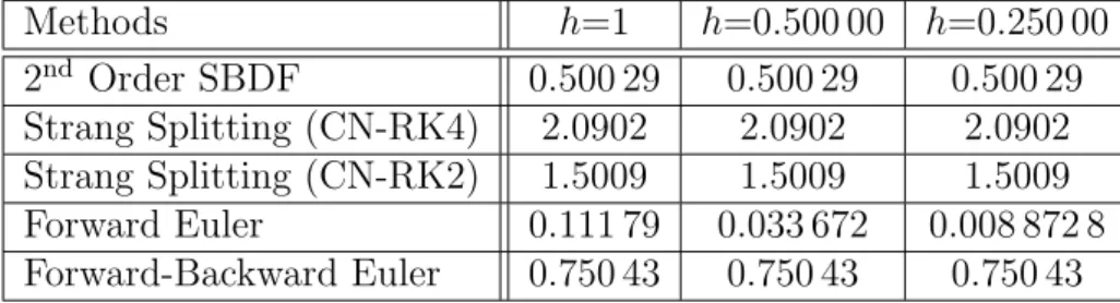
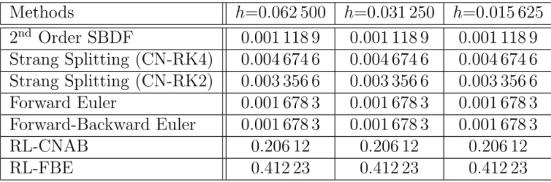
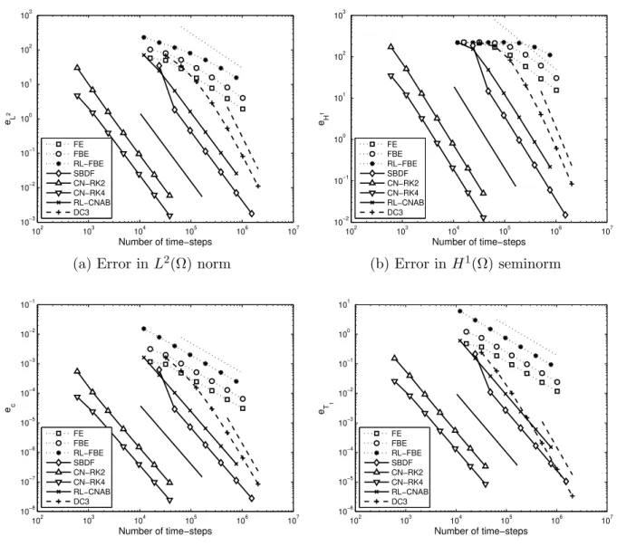
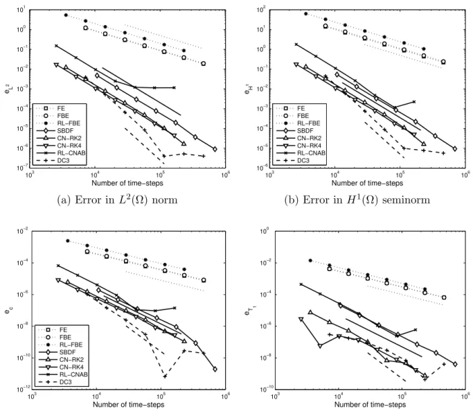
Analysis of time-stepping methods for the monodomain model

Using a convenient and readily parallelizable block-based approach, different regions of the fluid are assigned differing time steps and solved at different rates to

semigroup; Markov chain; stochastic gradient descent; online principle component analysis; stochastic differential equations.. AMS

The main conclusion from the analysis presented in this paper is that the numer- ical error in the projection method has the same structure as in the semi-discrete case (analyzed

The analysis is extended also to the case of fully discrete schemes, i.e., the combination of Galerkin time stepping methods with discretization in space.. For simplicity we do

Learners when developing their oral communication in a foreign language learning classroom need to structure, plan meaningful tasks and experiences within this

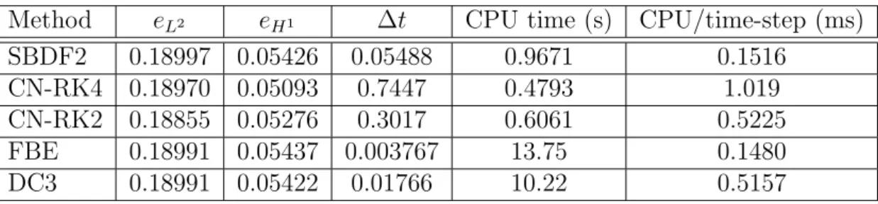
Efficient High Order Schemes for Stiff ODEs in Cardiac Electrophysiology

Below: comparison of the activation time mappings predicted by the bidomain (left) and adapted monodomain (right) models, on the finest mesh and also for χ = 1500 cm −1.. the

Однако ряд особенностей алгоритмов, видных лишь при сопоставлении разных методов решения одной и той же задачи, стал виден только по мере